Can oil prices predict the direction of exchange rate movements? An empirical and economic analysis for the case of India

Abstract

This study investigates whether oil prices have enough predictive information to predict the direction of the movement of exchange rate by examining the type of cointegration relationship between exchange rate and oil prices in India between 1991Q1 and 2013Q1. Our findings suggest the existence of cointegration relationship between exchange rate and oil prices using both Engle–Granger two-step cointegration test and Johansen cointegration test. Using a momentum threshold autoregressive consistent model, we find evidence in favour of asymmetric cointegration between the two variables. Nevertheless we find no evidence to support asymmetric cointegration relationship between the two variables when threshold autoregressive, threshold autoregressive consistent, and momentum threshold autoregressive models are used. Thus, the results suggest that for certain time period, the adjustment process between exchange rate and oil price is constant, which makes it conducive for predicting the direction of exchange rate movement. However, evidence of asymmetric cointegration suggests that the stable relationship is likely to be interrupted with intervals of structural change implying correction in the dynamics of influencing factors.

Keywords:

• Asymmetric cointegration
• exchange rate
• oil prices
• India

JEL CLASSIFICATION:

• C22
• E31

1. Introduction

Oil is among the most important commodities traded in the world. It has many uses including as a source of energy, raw material in various industries and trading commodity on which many financial derivatives are based. However, its price is primarily determined by market forces and as a result, research in price variability is common. This variability characteristic exerts a substantial impact on both the imports and exports of its major consumers and producers, thereby creating a consequential effect on their exchange rates. As a result, this phenomenon provokes interest in investigating the relationship between oil prices and exchange rates. Explicitly, this article analyses changes in the time series properties of oil prices and exchange rates in India over the last two decades in an attempt to shed light on two main research questions. Firstly, are oil prices and exchange rates cointegrated with adjustment process constant? And secondly, can oil prices predict the direction of exchange rate movement? By addressing these research questions we aim to improve our understanding of the relationship between oil prices and exchange rates in a way that will facilitate the formulation of more effective economic policies and monitoring mechanism for stabilising exchange rate.

Theoretical analysis of this relationship started with the work of Krugman (1983a) where he showed that the initial effects of an increase in oil prices on real exchange rates differ from their long-run effects. In the former it is an appreciation and in the latter it is depreciation. Further work by Krugman (1983b) proposes three models to explain the effects of oil shocks on exchange rates. The models suggest that oil shocks affect all countries, but their effects on the exchange rate depend on the asymmetries between the economies. Golub (1983), on the other hand, developed a flow model that looks into the effects of oil shocks on exchange rates, and concludes that the effects depend on the resultant direction which the individual countries will take in reallocating their wealth.

Empirical literature focuses more dominantly in this area, with most of the studies focusing on either single or several oil producing economies. The work of Corden (1984), Amano and Van Norden (1998) and Issa, Lafrance, and Murray (2008) are on individual country, whereas those of Arteta, Kamin, and Vitanza (2011) and Mundaca (2013) are on several oil producing countries. Issa et al. (2008) studied the relationship between energy prices and the Canadian dollar. Amano and Van Norden (1998) investigated and found evidence of a long-run relationship between oil prices and the US dollar exchange rates with respect to several major currencies. However, these studies have largely overlooked the fact that the adjustment speed for cointegrating (long run) relationship may not be constant. In addition, these studies also overlook the effects that changes in oil prices could have on large developed economies that are dependent on oil imports or countries that are currently both large oil producers and consumers.

Furthermore, theoretical models suggest that adjustment speed between these two series could be asymmetric. Apart from this, it has also been found that foreign exchange interventions as well as other monetary policies used by countries in order to influence the behaviour of their exchange rates generate asymmetries, which could be better modelled using non-linear techniques. However, most of the empirical literature uses linear models that include the Johansen cointegration and the Engle-Granger approach. Such linear models ignore the implications of monetary authorities’ aversion to large changes in exchange rates as verified by research on exchange rate regime. As for the use of non-linear techniques, there is literature such as the paper by Mohammadi and Jahan-Parvar (2012) in which threshold cointegration is used to investigate dynamics between the oil prices and exchange rates of Mexico, Norway and Bolivia. However, the study by Ahmad and Hernandez (2013) attracts much of our attention. In their research on the cointegrating relationship between oil prices and exchange rate for 11 countries and the euro area (which consists of 17 European countries), the authors find evidence of the existence of cointegration in six of the countries covered, while signs of asymmetric adjustments are detected in Brazil, the eurozone countries, Nigeria and the UK. The results indicate that Brazil, Nigeria and the UK record higher adjustment after a positive shock than after a negative shock. This means real exchange rate appreciation following a rise in the real oil prices is eliminated faster than a depreciation following a fall in the real oil prices. However, the results for the eurozone show the opposite trend in which adjustment is faster after a negative shock than after a positive shock. In addition, results for Brazil and the UK indicate Granger causality effect with respect to the real oil prices.

Additionally a number of papers have argued on the relationship between oil price and exchange rate from the perspective of wealth and expenses. An increase in the exchange rate of the US dollar means greater wealth for oil exporting economies and thus could drive up demand for imported goods, thus the demand for US dollars for settlement of the imports. For oil importers, the opposite effects will occur. The work of Al-Abdulhadi (2014) on demand for oil products in the Middle East countries reflects the aforementioned concept. Similar in line, Sodeyfi and Katircioglu (2016) found that oil price has a negative and positive impact on business activities. Anoruo and Elike (2009) found cointegration between oil price and economic growth in oil importing African countries. Shaeri and Katircioğlu (2018) found that there is long-run relationship between stock indices, crude oil price, short-term interest rate and the Standard & Poor’s 500. Gokmenoglu, Bekun and Taspinar (2016) concluded that there exists a long-run relationship between agricultural, economic growth, oil rent, and oil production. Shaeri, Adaoglu and Katircioglu (2016) concluded that the magnitude of oil price impact on the financial sector is lower than the non-financial subsector. Similarly, Katircioglu, Ozatac and Taspinar (2018) found that oil price bring negative impact on bank profitability in Turkey.

A large body of literature has been developed in investigating the relationship between oil price and exchange rate, applying different methods and sample countries. However, most of these empirical studies have assumed the symmetric relationship between oil prices on exchange rate and only a small portion of these literature investigated the existence of asymmetric relationship. This study aims to shed more light on asymmetric cointegration and investigate how it can be used to predict direction of exchange rate movement. In real situations, the relationship between oil price and exchange rate may be asymmetric. This article uses a methodology similar to the research approach of Ahmad and Hernandez (2013) but focusing more on the asymmetric cointegrating relationship between oil prices and exchange rates in India. In addition, this article also examines the implications of asymmetric cointegrating relationship on estimating the direction of exchange rate movement and subsequently policy action. India is chosen for this study based on two reasons. First, it is among the fastest growing economies in the world at this point of time. In addition, oil import makes up about 40% of India’s total imports while all transactions of oil are done in US dollar. Hence the relationship between oil price and exchange rate is tremendously important to the Indian economy as a whole. The rest of the article is planned as follows. Section 2 describes the Indian context especially on the asymmetric relationship between oil prices and exchange rate of India. Section 3 describes the data and methodologies that will be applied in this study. Section 4 presents the empirical results while Section 5 concludes this article.

2. The Indian context

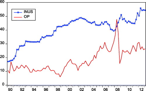
India is known to be the fourth largest oil importer in the world and it imports in excess of three million barrels of petroleum per day. Over the fiscal period from 2006 to 2011, on average, crude oil took up about 40% of the country’s annual total imports. Surprisingly, in the fiscal year 2011–2012, oil import climbed up to over 53% of the total imports, making an increase of 13% just in one year, worth a staggering US$160 billion in monetary value. One of the obvious reasons for this increase is the upsurge in the use of modern technology in production of both agricultural as well as non-agricultural sectors, including a phenomenal rise in the use of the modern mode of transport such as automobiles and motorbikes. These are phenomena associated with rapid economic growth, while oil is a necessary energy source for national economic development. Another contributing factor is the rising crude oil price in the international market (see Figure 1). Given that the demand for petroleum is relatively inelastic, an increase in the price of petroleum has significantly increased the amount spent on imports. Moreover, practically all oil contracts are denominated in US dollars in the world market. Therefore, a change in the price of oil can have a significant impact on the demand as well as supply of foreign exchange. This warrants an in-depth study on how the rate of real exchange rate appreciation or depreciation is eliminated following a rise or fall in the real oil prices.

Figure 1. The India rupee to US dollar exchange rate (INUS) and oil prices (OP).

Source: Organisation for Economic Co-operation and Development (OECD).

3. Data and methodologies

This study uses the quarterly data to estimate the link between oil prices and exchange rate. Though using monthly or daily data makes better econometric sense, in reality, it is very unlikely oil prices can appear as high frequency data simply because it needs more time for production. Moreover, there is a substantial amount of literature which uses quarterly data; for example Clarida and Gali (1994) and Coudert, Mignon, and Penot (2008). In addition, oil prices are usually used together with other macro variables like GDP, which are usually used in quarterly data for analysis and forecasting. Therefore, based on the reasons explained above, this study employs quarterly data from the period 1991:Q1 to 2013:Q1 for India. The variables are the exchange rate (ER): $\frac{\mathit{\text{INRUS}}\mathrm{\hspace{0.17em}*\hspace{0.17em}}{CPI}^{US}}{{CPI}^{INR}}$ and the oil price (OP): $\frac{\mathit{\text{OilPrice}}\mathrm{\hspace{0.17em}*\hspace{0.17em}}\mathit{\text{INRUS}}}{{CPI}^{INR}}$ where the real bilateral exchange rate refers to that from the Indian rupee (INR) to US dollars. Both the exchange rate (ER) and oil price (OP) use US dollar as measurement unit. Data are obtained from the Organisation for Economic Co-operation and Development (OECD). All variables are transformed into natural logarithms prior to estimation. The exchange rate series is seasonally adjusted.

3.1. Engle–Granger cointegration tests

Following Chaudhuri and Daniel (1998), the bivariate equation between exchange rate and oil price is written as: (1) $${LER}_t={\alpha }_0+{\alpha }_1{LOP}_t+u_t$$(1) where ${LER}_t$ and ${LOP}_t$ denote the log exchange rate and the log oil price respectively, ${\alpha }_0$and ${\alpha }_1$ are parameter estimates and $u_t$ is residuals term. The residuals of the linear regression ($u_t$) are then tested for stationarity using ADF unit root tests. Equation (2)(2) $$\Delta {\widehat{u}}_t=p{\widehat{u}}_{t-1}+v_t$$(2) shows the basic unit root test model. (2) $$\Delta {\widehat{u}}_t=p{\widehat{u}}_{t-1}+v_t$$(2)

3.2. Enders–Siklos (ES) asymmetric cointegration tests

If ${LER}_t$ and ${LOP}_t$ are cointegrated, then there exists a long-run equilibrium relationship between these variables in India. However, this cointegration relationship may not be symmetrical simply because of government interventions in the exchange rate market. Hence we need to explore the possibilities of asymmetries in the adjustment process with the application of threshold autoregressive (TAR) and momentum threshold autoregressive consistent (MTAR) models. In general, standard cointegration tests follow the assumption of symmetric adjustment (Engle & Granger, 1987). However, Engle and Granger tests are mis-specified when the exchange rate and oil price have asymmetric relationship (Enders & Siklos, 2001). Taking into consideration the possibility of asymmetries in the process of error correction, the adjustment of oil price to changes in the exchange rate in the long run is as represented in Equation (3)(3) $$\mathbf{\Delta }{\widehat{u}}_t=I_t{p}_1{\widehat{u}}_{t-1}+\left(1-I_t\right)p_2{\widehat{u}}_{t-1}+\sum _{i=1}^p{\gamma }_i\mathbf{\Delta }{\widehat{u}}_{t-1}+{ϵ}_t$$(3) : (3) $$\mathbf{\Delta }{\widehat{u}}_t=I_t{p}_1{\widehat{u}}_{t-1}+\left(1-I_t\right)p_2{\widehat{u}}_{t-1}+\sum _{i=1}^p{\gamma }_i\mathbf{\Delta }{\widehat{u}}_{t-1}+{ϵ}_t$$(3) where $$I_t=[T_t,M_t]$$ such that, (4) $$T_t=\left\{\begin{array}{l}1if{\widehat{u}}_{t-1}\ge \tau \\ 0if{\widehat{u}}_{t-1}<\tau \end{array}\right.$$(4) (5) $$M_t=\left\{\begin{array}{l}1if{\mathbf{\Delta }\widehat{u}}_{t-1}\ge \tau \\ 0if{\mathrm{}\mathbf{\Delta }\widehat{u}}_{t-1}<\tau \end{array}\right.$$(5) where $\tau$ is threshold. The TAR and MTAR models can be estimated using the initial threshold values set to zero as shown in Equations (3)–(5). The analysis is then continued to search for the consistent estimate of the threshold values by using Chan’s (1993) approach.

3.3. Asymmetric error correction modelling

Given the existence of cointegration between the exchange rate and oil price and also asymmetric adjustment in the context of MTAR Consistent model, asymmetric error-correlation models are as shown in Equations (6)(6) $$\mathbf{\Delta }{LER}_t={\alpha }_0-{\theta }_{11}{M}_t{u}_{t-1}-{\theta }_{12}\left(1-M_t\right)u_{t-1}+\sum _{i=1}^k{\alpha }_{1i}\mathbf{\Delta }{LER}_{t-i}+\sum _{i=1}^k{\alpha }_{2i}\mathbf{\Delta }{LOP}_{t-i}+{ϵ}_{1t}$$(6) and (7)(7) $$\mathbf{\Delta }{LOP}_t={\beta }_0-{\theta }_{21}{M}_t{u}_{t-1}-{\theta }_{22}\left(1-M_t\right)u_{t-1}+\sum _{i=1}^k{\beta }_{1i}\mathbf{\Delta }{LER}_{t-i}+\sum _{i=1}^k{\beta }_{2i}\mathbf{\Delta }{LOP}_{t-i}+{ϵ}_{2t}$$(7) : (6) $$\mathbf{\Delta }{LER}_t={\alpha }_0-{\theta }_{11}{M}_t{u}_{t-1}-{\theta }_{12}\left(1-M_t\right)u_{t-1}+\sum _{i=1}^k{\alpha }_{1i}\mathbf{\Delta }{LER}_{t-i}+\sum _{i=1}^k{\alpha }_{2i}\mathbf{\Delta }{LOP}_{t-i}+{ϵ}_{1t}$$(6) (7) $$\mathbf{\Delta }{LOP}_t={\beta }_0-{\theta }_{21}{M}_t{u}_{t-1}-{\theta }_{22}\left(1-M_t\right)u_{t-1}+\sum _{i=1}^k{\beta }_{1i}\mathbf{\Delta }{LER}_{t-i}+\sum _{i=1}^k{\beta }_{2i}\mathbf{\Delta }{LOP}_{t-i}+{ϵ}_{2t}$$(7) where ${\theta }_{11}$ and ${\theta }_{12}$ are the parameters of speed of adjustment for $\mathbf{\Delta }{LER}_t$ if above and below its long run equilibrium respectively, while ${\theta }_{21}$ and ${\theta }_{22}$ are the speed of adjustment coefficients of $\mathbf{\Delta }{LOP}_t$ if above and below its long-run equilibrium correspondingly. ${\alpha }_0$ and ${\beta }_0$ are constant terms. ${\alpha }_{1i}$, ${\alpha }_{2i}$, ${\beta }_{1i}$ and ${\beta }_{2i}$ are the coefficients of lagged change terms. The white-noise disturbances are ${ϵ}_{1t}$ and ${ϵ}_{2t}$.

4. Empirical results

Table 1 indicates that ${LER}_t$ and ${LOP}_t$ are non-stationary at levels, but stationary at the first-differences, suggesting that these variables are integrated of order one, I(1) process. Subsequently, we examine the possibilities of cointegration (long-run) relationship between exchange rate (${LER}_t$) and oil price (${LOP}_t$) in India using ordinary least squares (OLS) as presented in Table 2.

Table 1. Unit root tests.

	Augmented Dickey–Fuller (ADF)		Phillips–Perron (PP)
	Level
Variable	Constant without trend	Constant with trend	Constant without trend	Constant with trend
LERt	−1.335(0)	−2.654(0)	−1.637[4]	−2.678[2]
LOPt	−1.835(0)	−3.254(0)	−1.823[1]	−3.324[1]
	First difference
ΔLERt	−7.961(0)***	−8.354(0)***	−8.067[2]***	−8.413[2]***
ΔLOPt	−10.083(0)***	−10.027(0)***	−10.218[4]***	−10.151[4]***

*** Significance at 1% level. The figures in parentheses () and [] indicate the optimal lag length or bandwidth used for ADF and PP tests, respectively. The maximum lag length for ADF tests is selected using the akaike information criteria (AIC), whereas truncation lags are for the Newey–West bandwidth criterion of the PP test.

Table 2. Cointegration regression.

Variable	Dependent: LERt
Constant	1.813	(−51.016)***
LOPt	−0.148	(−5.134)***

*** Significance at the 1% level. The figure in parenthesis represents t-statistic.

Table 2 presents the long run regression as follows: (8) $$\stackrel{⁁}{{LER}_t}=1.813-0.{\text{148}LOP}_t$$(8)

According to the long-run regression, increase in oil price will weaken the exchange rate of the Indian rupee to US$. This relationship is in line with the results of past studies (Chen & Chen, 2007). An explanation for this relationship is that, India is a heavy oil importer country; thus, higher oil price (traded in US dollars) will increase the demand for US dollars and thereby depreciates the exchange rate in favour of the US dollar. This will result in the price increase of tradable compared to non-tradable and the depreciation of the Indian rupee/US dollars exchange rate.

Next, the residual (u_t) will be employed to estimate in the Engle–Granger (EG) cointegration test. The cointegration test is further applied to confirm the long-run relation between ${LER}_t$ and ${LOP}_t$. This can be done by detecting the presence of a unit root (no cointegration) in the residuals. The results summarised in Table 3 show that the null hypothesis of no cointegration is rejected at 1% level of significance. This suggests that the examined variables are cointegrated implying there exists a long-run relationship between these variables in India.

Table 3. Engle–Granger (EG) cointegration test.

Variable	Dependent: $\Delta u_t$
$u_{t-1}$	−2.638 [0]	(−0.009)***

*** Significant at the 1% level. The figures in parentheses () and [] represent t-statistic and optimum lag length respectively. The maximum lag length is selected using the AIC.

After the Engle–Granger two-step cointegration test, Enders–Siklos asymmetric cointegration test is applied to investigate the asymmetric cointegration. The empirical results of TAR and MTAR models are reported in Table 4. Based on the TAR and MTAR models, the value of the threshold is zero, which is deterministic in nature, and it is imposed through regressing the original series on a constant for deriving a new series. In reality, the threshold value considers a non-zero. Therefore, the method of Chan (1993) is applied to search for the threshold value for TAR-consistent and MTAR-consistent, the threshold value in TAR-consistent is –0.067 and MTAR-consistent is 0.023. We fail to reject the null hypothesis of no cointegration (${\widehat{p}}_1={\widehat{p}}_2=0$) in TAR, TAR-consistent and MTAR models. These findings suggest that no cointegration exists between the exchange rate (${LER}_t$) and oil price (${LOP}_t$). Alternatively, MTAR-consistent model rejects the null hypothesis of ${\widehat{p}}_1={\widehat{p}}_2=0$ at the 5% level. However, the exchange rate and oil price have been verified to be cointegrated. This discrepancy in cointegration results warrants an examination of the possibility of asymmetry adjustment. Based on the standard F-statistic = 8.792 in MTAR consistent model, we reject the symmetric adjustment null at 5% level.

Table 4. Asymmetric cointegration tests using 0 threshold and consistent threshold.

	TAR	TAR-consistent	MTAR	MTAR-consistent
${\widehat{p}}_1$	−0.119(−1.714)	−0.099(−1.595)	−0.196(−2.641)	−0.595(−3.683)
${\widehat{p}}_2$	−0.149(−2.363)	−0.185(−2.547)	−0.096(−1.602)	−0.101(−2.138)
${\gamma }_1$	0.105(1.001)	0.093(0.881)	0.111(1.067)	0.118(1.179)
${\gamma }_2$	−0.052(−0.516)	−0.058(−0.576)	−0.049(−0.494)	−0.046(−0.484)
${\gamma }_3$	0.195(1.942)	0.193(1.928)	0.195(1.951)	0.218(2.280)
$\tau$	0.000	−0.067	0.000	0.023
${\widehat{p}}_1={\widehat{p}}_2=0$	4.061	4.45	4.618	8.816**
${\widehat{p}}_1={\widehat{p}}_2$	0.106	0.817	1.124	8.792**

** Significant at 5% level. The figures in parentheses represent t-statistic. The critical values are obtained from Monte Carlo experiment. The optimal lag length is selected using specific to general approach with a maximum of up to eight lags.

Under MTAR-consistent specification (Equation 9(9) $$\begin{array}{l}\Delta \stackrel{⁁}{{LER}_t}=0.0003-0.4450I_t{\widehat{u}}_{t-1}-0.0772\left(1-I_t\right){\widehat{u}}_{t-1}+B_{11}\Delta LE{R}_{t-1}+B_{12}\Delta LO{P}_{t-1}\\ \left(0.195\right)(-3.708)***(-2.224)***F_{11}<0.01F_{12}<0.01\end{array}$$(9) ), the parameter estimates for ${\theta }_{11}$ and ${\theta }_{12}$ appear to have a negative sign and statistically significant at 1%, suggesting that the short-run disequilibrium converges to the long-run equilibrium through asymmetric adjustments. Moreover, the speed of adjustment is 44.50% when the exchange rate is above the threshold value for a decrease in the oil price. Conversely, the speed of adjustment is 7.72% when the exchange rate is below the threshold value for an increase in the oil price. The speed of adjustment of the exchange rate to an increase in the oil price is slower than when the oil price decreases. Under MTAR-consistent specification (equation 10(10) $$\begin{array}{l}\Delta \stackrel{⁁}{{LOP}_t}=0.0075-0.7292I_t{\widehat{u}}_{t-1}-0.1183\left(1-I_t\right){\widehat{u}}_{t-1}+B_{21}\Delta LE{R}_{t-1}+B_{22}\Delta LO{P}_{t-1}\\ \left(1.009\right)(-1.297)(-0.662)F_{21}<0.10F_{22}<0.05\end{array}$$(10) ), however, both the asymmetric error correction terms ${\theta }_{21}$ and ${\theta }_{22}$ are insignificant at conventional level. Thus, oil price is exogenous to the exchange rate. (9) $$\begin{array}{l}\Delta \stackrel{⁁}{{LER}_t}=0.0003-0.4450I_t{\widehat{u}}_{t-1}-0.0772\left(1-I_t\right){\widehat{u}}_{t-1}+B_{11}\Delta LE{R}_{t-1}+B_{12}\Delta LO{P}_{t-1}\\ \left(0.195\right)(-3.708)***(-2.224)***F_{11}<0.01F_{12}<0.01\end{array}$$(9) (10) $$\begin{array}{l}\Delta \stackrel{⁁}{{LOP}_t}=0.0075-0.7292I_t{\widehat{u}}_{t-1}-0.1183\left(1-I_t\right){\widehat{u}}_{t-1}+B_{21}\Delta LE{R}_{t-1}+B_{22}\Delta LO{P}_{t-1}\\ \left(1.009\right)(-1.297)(-0.662)F_{21}<0.10F_{22}<0.05\end{array}$$(10)

Table 5 shows the results for diagnostic checking. The MTAR-consistent model (Equation 9(9) $$\begin{array}{l}\Delta \stackrel{⁁}{{LER}_t}=0.0003-0.4450I_t{\widehat{u}}_{t-1}-0.0772\left(1-I_t\right){\widehat{u}}_{t-1}+B_{11}\Delta LE{R}_{t-1}+B_{12}\Delta LO{P}_{t-1}\\ \left(0.195\right)(-3.708)***(-2.224)***F_{11}<0.01F_{12}<0.01\end{array}$$(9) ) reveals that the model is normally distributed; no serial correlation and no ARCH effects in the residuals.

Table 5. Diagnostic checking.

AR(1)	ARCH(1)	Jarque-Bera
1.187(0.279)	1.006(0.319)	2.182(0.336)

Note: AR(1) is Breush–Godfrey serial LM test; ARCH (1) is autoregressive conditional heteroscedasticity test; Jarque–Bera is normality test.

Tables 6 and 7 show the Dicky–Fuller generalised least square (DG-GLS) and Ng and Perron (2001) unit root test results confirming the test results as shown in Table 1. On the other hand, the results of Johansen (1988) cointegration test results in Table 8 support the results in Table 3. Lastly, the cumulative sum of recursive residual (CUSUM) test (Figure 2) provides strong support of stability in parameter estimates, indicating that the model is stable over the sample period.

Figure 2. CUSUM test.

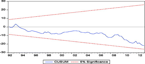
Table 6. Unit root tests for Dicky–Fuller generalised least square (DG-GLS).

	DG-GLS
	Level
Variable	Constant without trend	Constant with trend
LERt	−0.939(0)	−1.039(0)
LOPt	−1.539(0)	−3.522(0)
First Difference
ΔLERt	−8.259(0)***	−8.565(0)***
ΔLOPt	−3.004(2)***	−9.024(0)***

Notes: * Elliott, Rothenberg, and Stock (1996, Table 1). The figures in parentheses () indicates the optimal lag length or bandwidth used for DG-GLS. The maximum lag length for DG-GLS tests is selected using the Schwarz information criterion.

Table 7. Unit root tests for Ng, and Perron.

Ng & Perron at level
Variables	Mza	Mzt	MSB	MPT
LER	−1.719	−0.898	0.523	13.807
LOP	−5.272	−1.481	0.281	5.031
Ng & Perron at 1^st difference
LER	−44.632*	−4.723	0.106	0.549
LOP	−31.216*	−3.937	0.126	0.828

Note: * Ng & Perron (2001, Table 1).

Table 8. Johansen (1988) cointegration test.

Null	Alternative	Maximum Eigen statistic		Trace statistic
		Statistics	95% critical value	Statistics	95% critical value
R = 0	R = 1	16.523**	14.265	16.983**	15.495
R ≤ 1	R = 2	0.459	3.841	0.459	3.841

Note: *, **, and *** denotes statistically significant at 10%, 5% and 1% respectively.

5. Conclusion

The study aims to examine cointegration and asymmetric cointegration relationship between exchange rate and oil prices in India from 1991:Q1 to 2013:Q1 using a battery of TAR, TAR-consistent and MTAR models. The findings suggest the existence of cointegration relationship between exchange rate and oil prices using Engle–Granger two-step cointegration test. However, we also find evidence in favour of asymmetric cointegration between exchange rate and oil prices in MTAR-consistent test, but there is no evidence to support asymmetric cointegration between the two variables examined using TAR, TAR-consistent and MTAR models. The results are intuitively appealing and explain ambiguity in the adjustment process between exchange rate and oil prices. Therefore, we can conclude that there exist adjustment processes between exchange rate and oil price, indicating the appreciation of exchange rate may be wiped out faster when oil prices go up than when oil prices fall. Hence, when the oil price increases, the government needs to intervene in the foreign exchange market fast so as to stabilise exchange rate volatility. However, when the oil price falls, intervention can be done at a more leisurely pace. These steps are necessary because of the asymmetric effect of cointegration.

Since India is a net oil importer, it has no absolute influence on the international market price of oil, while the elasticity of oil demand could have an effect on the exchange rate. On the other hand, oil represents a critical input for national economic development. Therefore, an investigation on the nexus of the dynamics of oil demand elasticity, oil price movement and economic growth could potentially provide insight that will be useful to policy-makers in the process of aligning the exchange rate of the Indian rupee, particularly in balancing out the negative impact of rising oil prices on economic growth.

In summary, the finding of symmetric and asymmetric conditions in our results shows that there is a stable relationship between oil price and exchange rate, but there exist windows when the relationship will be otherwise influenced. This implies that policy-makers in examining the oil price–exchange rate relationship should also take into account the influence of significant events during the period of structural change.

Even though the relationship between oil price and exchange rate has been investigated many times, there is still space for this type of research whereby we can always attempt to trace out the short time period of constancy in adjustment speed and investigate whether any suitable method of tracing the time period can be applied to both developed and developing economies.

Disclosure statement

No potential conflict of interest was reported by the authors.

References

- Anoruo, E., & Elike, U. (2009). An empirical investigation into the impact of high oil prices on economic growth of oil-importing african countries. International Journal of Economic Perspectives, 3, 121–129.
- Al-Abdulhadi, D. J. (2014). An analysis of demand for oil products in Middle East countries. International Journal of Economic Perspectives, 8, 5–12.
- Ahmad, A. H., & Hernandez, R. M. (2013). Asymmetric adjustment between oil prices and exchange rates: Empirical evidence from major oil producers and consumers. Journal of International Financial Markets, Institutions and Money, 27, 306–317. doi: 10.1016/j.intfin.2013.10.002
- Amano, R. A., & Van Norden, S. (1998). Oil prices and the rise and fall of the US real exchange rate. Journal of International Money and Finance, 17(2), 299–316. doi: 10.1016/S0261-5606(98)00004-7
- Arteta, C., Kamin, S. B., & Vitanza, J. (2011). The puzzling peso. Journal of International Money and Finance, 30(8), 1814–1835. doi: 10.1016/j.jimonfin.2011.09.002
- Chan, K. S. (1993). Consistency and limiting distribution of the least squares estimator of a threshold autoregressive model. The Annals of Statistics, 21(1), 520–533. doi: 10.1214/aos/1176349040
- Chaudhuri, K., & Daniel, B. C. (1998). Long-run equilibrium real exchange rates and oil prices. Economics Letters, 58(2), 231–238. doi: 10.1016/S0165-1765(97)00282-6
- Chen, S. S., & Chen, H. C. (2007). Oil prices and real exchange rates. Energy Economics, 29(3), 390–404. doi: 10.1016/j.eneco.2006.08.003
- Clarida, R., & Gali, J. (1994). Sources of real exchange-rate fluctuations: How important are nominal shocks? Carnegie-Rochester Conference Series on Public Policy, 41, 1–56. doi: 10.1016/0167-2231(94)00012-3
- Coudert, V., Mignon, V., & Penot, A. (2008). Oil price and the dollar. Energy Studies Review, 15, 45–58.
- Corden, W. M. (1984). Booming sector and Dutch disease economics: Survey and consolidation. Oxford Economic Papers, 36(3), 359–380. doi: 10.1093/oxfordjournals.oep.a041643
- Elliot, G., Rothenberg, T. J., & Stock, J. H. (1996). Efficient tests for an autoregressive unit root. Econometrica, 64, 813–836. doi: 10.2307/2171846
- Enders, W., & Siklos, P. L. (2001). Cointegration and threshold adjustment. Journal of Business & Economic Statistics, 19, 166–176. doi: 10.1198/073500101316970395
- Engle, R. F., & Granger, C. W. J. (1987). Co-integration and error correction: Representation, estimation, and testing. Econometrica, 55(2), 251–276. doi: 10.2307/1913236
- Gokmenoglu, K. K., Bekun, F. V., & Taspinar, N. (2016). Impact of oil dependency on agricultural development in Nigeria. International Journal of Economic Perspectives, 10, 151–163.
- Golub, S. S. (1983). Oil prices and exchange rates. The Economic Journal, 93(371), 576–593. doi: 10.2307/2232396
- Issa, R., Lafrance, R., & Murray, J. (2008). The turning black tide: Energy prices and the Canadian dollar. Canadian Journal of Economics/Revue Canadienne D'économique, 41(3), 737–759. doi: 10.1111/j.1540-5982.2008.00483.x
- Johansen, S. (1988). Statistical analysis of cointegration vectors. Journal of Economic Dynamics and Control, 12, 231–254. doi: 10.1016/0165-1889(88)90041-3
- Katircioglu, S., Ozatac, N., & Taspinar, N. (2018). The role oil prices, growth and inflation in bank profitability. The Service Industries Journal, 20, 1–20
- Krugman, P. R. (1983a). Oil and the dollar. In Bhandari, J. S., Putnam, B. H. (Eds), Economic Interdependence and Flexible Exchange Rates (179-190). Cambridge: Cambridge University Press.
- Krugman, P. R. (1983b). Oil shocks and exchange rate dynamics. In Frankel, J. A. (Ed.), Exchange Rates and International Macroeconomics (259-284). Chicago: University of Chicago Press.
- Mohammadi, H., & Jahan-Parvar, M. (2012). Oil prices and exchange rates in oil-exporting countries: Evidence from TAR and M-TAR models. Journal of Economics and Finance, 36(3), 766–779. doi: 10.1007/s12197-010-9156-5
- Mundaca, G. (2013). Oil prices and exchange rate volatility in Arab countries. Applied Economics Letters, 20(1), 41–47. doi: 10.1080/13504851.2012.674200
- Ng, S., & Perron, P. (2001). Lag length selection and the construction of unit root test with good size and power. Econometrica, 69(6), 1519–1554. doi: 10.1111/1468-0262.00256
- Sodeyfi, S., & Katircioglu, S. (2016). Interactions between business conditions, economic growth, and crude oil prices. Economic Research - Ekonomska Istraživanja, 29(1), 980–990. doi: 10.1080/1331677X.2016.1235504
- Shaeri, K., Adaoglu, C., & Katircioglu, S. (2016). Oil price risk exposure: A comparison of financial and non-financial subsectors. Energy, 109, 712–723. doi: 10.1016/j.energy.2016.05.028
- Shaeri, K., & Katircioğlu, S. (2018). The nexus between oil prices and stock prices of oil, technology and transportation companies under multiple regime shifts. Economic Research - Ekonomska Istraživanja, 31(1), 681–702. doi: 10.1080/1331677X.2018.1426472