How much does regional integration contribute to growth? An analysis of the impact of domestic market integration on regional economic performance in China (1997–2011)

Abstract

This study analyses domestic market integration’s (DMI’s) dynamic influence on regional economic growth in China. The authors construct a matrix of annual DMI indices for 29 provinces for 1997–2015. They calculate the reciprocal matrix and combine it with the β-convergence model and spatial econometrics to analyse the relationships between DMI and regional economic growth. Their findings indicate that the relation between these two variables is not straightforward, and 2004 was a tipping-point year. Before 2004, the statistical relationship between DMI and regional economic growth was downward sloping, which suggests a trend of divergence and negative spillover effects across the 29 provinces. After 2004, the relationship between DMI and regional economic growth becomes positive: increased DMI now is strengthening (regional) economic growth. The authors provide the possible explanations for the unstable relationship combined with China’s reality as well.

Keywords:

• β-convergence
• economic growth
• market integration
• spatial autoregressive model
• spatial error model

JEL CLASSIFICATIONS:

• Q18
• P25
• N15

1. Introduction

How much did regional integration contribute to China’s successful economic performance in recent decades? This question takes on particular importance, if only because China’s sheer geographic size and rugged topography mean there are significant physical barriers to regional domestic market integration (DMI) which hinder the exploitation of regional specialisation and limit the gains from inter-regional trade (Poncet, 2005). Did China’s market-oriented reforms lead to a reduction in regional fragmentation, increased cross-regional flow of goods, capital and labour, and higher (regional) economic growth? This question has been addressed by a large and growing literature on the regional dimensions of China’s economic growth miracle (e.g., Bai, Ma, & Pan, 2012; Ke, 2015; Lu & Chen, 2006).

This paper complements the extant literature by using a novel network approach to analyse the role DMI is playing in the process of regional economic growth in a panel of 29 Chinese provinces during 1997–2015. Few studies view regions as a network, a typical characteristic of which can virtually reflect not only local relations but also the global state of regions. We develop a matrix of regional integration in which each entry is an index representing the level of market integration between a given pair of regions. This matrix represents a network configuration and its nodes and links are the provinces and indices of market integration. The reciprocal of this (original) matrix is combined with methods of spatial econometrics to analyse the relationship between DMI and regional economic growth. The cut-off matrix (which is a binary version of our original matrix) is used to demonstrate the overall attributes of market integration in China using network graphs. The present study finds that the relationship between DMI and regional economic growth is reflected by a U-shaped curve. That is, our evidence suggests that while higher DMI was associated with lower regional economic growth in the first years (1997–2004), this changed during 2004–2015, when higher DMI is found to contribute to higher regional economic growth. Multiple factors influence the way DMI affects regional economic growth, including appropriate institutions and policies, the diversity of comparative advantage and an efficient transportation system. We argue that once these three factors are in place, DMI is likely to improve regional economic growth (as happened in China post-2004). Spatial spillover effects would be more pronounced through DMI as a transmission mechanism under these conditions.

The remainder of this paper has the following structure. Section 2 presents a brief review of the literature. Section 3 introduces empirical methods and describes the data used in the analysis. Section 4 constructs the network matrices and presents network graphs to reflect the dynamics of DMI in China from 1997 to 2015. Section 5 presents an econometric investigation using β-convergence models with market integration that identifies the impact of market integration on regional economic growth. Section 6 provides an explanation of why DMI started to improve regional economic growth in China after 2004. The final section presents our conclusions, and also highlights the limitations and avenues for future research.

2. Literature review

China has experienced rapid economic growth since 1979. According to the data from the Conference Board, the annual average growth rate of real gross domestic product (GDP) per capita was 9.20% during 1997–2015.¹ The determinants of such a high growth rate are an ongoing research topic. Among these factors, some studies highlight the growth-promoting impacts of institutional reforms (Qian, 2002; Woo, 1999), rapid accumulation of capital (Chow & Li, 2002; Wang & Yao, 2003), inflows of foreign direct investment (Bai, Lu, & Tao, 2010; Su & Liu, 2016), increases in human capital stock (Li & Liang, 2009; Li, Loyalka, Rozelle, & Wu, 2017), and substantial improvements in total factor productivity (Bosworth & Collins, 2008). However, most of these studies ignore the growth-enhancing impact of a deeper economic integration between Chinese provinces and basically assume that the economic performance of Chinese regions can be analysed in isolation from what happens in the other regions. Inter-regional relationships are known to play important roles in the process of national economic growth, as is shown by the following studies. Using exploratory spatial data analysis, Ying (2000) confirms the effects of spatial spillover in China from core-to-periphery regions, such as from Guangdong Province to its adjacent provinces. Brun, Combes, and Renard (2002) and Zhang and Felmingham (2002) document the existence of positive influences that coastal regions exert on inland regions. Using spatial error modelling, Bai et al. (2012) estimate that a 10% increase in market potential (i.e., an index measuring proximity to large markets) increases the growth rates of different regions’ GDP per capita by 3–5%. Scherngell, Borowiecki, and Hu (2014) find that there exists a shift of Chinese productivity growth towards a more knowledge-based one, and this shift is not only based on region-internal knowledge capital, but also on inter-regional knowledge spillovers. Sun, Chen, and Hewings (2017) show that spatial spillovers exist not only among the economic growth of neighbours, but also among the initial economic levels of neighbours. Some studies offer alternative explanations to these findings. For example, Ying (2003) finds spatial autocorrelation of inter-regional output to be negative, using provincial data from 1978 to 1998, and concludes that spatial autocorrelation is an important reason for polarising processes in regional economies. Lin, Long, and Wu (2006) find relatively lower dispersion in the economic development process of regions when they statistically control for spatial autocorrelation compared with when they do not do this.

Inter-regional trade is the prime inter-regional relationship and a major source of economic growth. However, trade delays and blockages to inter-regional trade can occur due to local governments in China adopting radically different policies concerning DMI. Findings by Young (2000) illustrate that such delays and blockages were serious during the early years of reform and openness. The following researchers confirm the persistent trend of market fragmentation, especially after the fiscal decentralisation reform in the early 1990s to various degrees (Lu & Chen, 2009). Poncet (2005) investigates market fragmentation at the industry level and concludes that although the central government promoted domestic market integration, inter-provincial trade intensity declined and locally produced goods supplied a growing share of provincial consumption to the detriment of goods produced in the rest of the country. During these years, on the one hand, large and small (by GDP) regional provinces in China enacted many distinctly different preferential policies to increase exports, such as reduction of taxes, reduced industrial land prices, and the simplification of approval procedures. On the other hand, the same provinces enacted distinctly restrictive policies to stop products produced by other domestic regions from entering local markets. Some of the policies were indirectly restrictive. For example, the departments of local governments were only allowed to buy local products if it was possible. Some of the policies were directly restrictive, forbidding products from other regions being sold in local markets. Administrators who broke the rules were punished in several ways (sometimes even in illegal ways). These policies’ enactments resulted in a paradoxical outcome: high integration in international markets and low integration in domestic markets coexisted in several large and small (measured by GDP) provinces in China. Poncet (2003) finds evidence for the period 1987–1997 to support this conclusion after analysing goods flow data extracted from China’s provincial input–output tables.

3. Method and data

3.1. The index of DMI

The present study estimates provincial variances of relative prices (PVRP) and uses this as an indicator of price convergence. If PVRP are declining, this is taken to reflect growing market integration. The iceberg cost model is the foundational theory supporting the study of PVRP (Samuelson, 1964). The iceberg cost model indicates that two markets are integrated if the variance of relative prices is restricted to a certain range. The empirical approaches of Parsley and Wei (2001) are widely used in the literature, and this paper follows their work and that of Lu and Chen (2006) to calculate the index of market integration in China using PVRP metrics. The computational process includes three steps.

Step 1: calculation of relative prices: (1) $$|\Delta Q^k{}_{i,j,t}\left| = \right|\hspace{0.17em}\text{ln}\hspace{0.17em}\left(P^k{}_{i,t}/ P^k{}_{j,t}\right) - \hspace{0.17em}\text{ln}\hspace{0.17em}\left(P^k{}_{i,t-1}/ P^k{}_{j,t-1}\right)$$(1) where P^k_i,t is the price of commodity k in region i and period t. We use the logarithmic form of relative price because this renders the observed values less volatile and reduces the influence of heteroscedasticity. We define relative prices in first-order difference to make explicit price convergence or divergence; if |ΔQ^k_i,j,t| > 0 relative prices between two provinces diverge, and vice versa. A declining |ΔQ^k_i,j,t| suggests greater DMI. We use the consumer price index by category and region as our price indicator; note that this is a kind of chain price index. The index is observable clearly by transforming Equation (1)(1) $$|\Delta Q^k{}_{i,j,t}\left| = \right|\hspace{0.17em}\text{ln}\hspace{0.17em}\left(P^k{}_{i,t}/ P^k{}_{j,t}\right) - \hspace{0.17em}\text{ln}\hspace{0.17em}\left(P^k{}_{i,t-1}/ P^k{}_{j,t-1}\right)$$(1) into Equation (2)(2) $$\left|\Delta Q^k{}_{i,j,t}\right| = |\hspace{0.17em}\text{ln}\hspace{0.17em}\left(P^k{}_{i,t}/P^k{}_{i,t-1}\right) - \hspace{0.17em}\text{ln}\hspace{0.17em}\left(P^k{}_{j,t}/P^k{}_{j,t-1}\right)$$(2) . (2) $$\left|\Delta Q^k{}_{i,j,t}\right| = |\hspace{0.17em}\text{ln}\hspace{0.17em}\left(P^k{}_{i,t}/P^k{}_{i,t-1}\right) - \hspace{0.17em}\text{ln}\hspace{0.17em}\left(P^k{}_{j,t}/P^k{}_{j,t-1}\right)$$(2)

Note that calculating the absolute value of |ΔQ^k_i,j,t| does exclude a consequence which is not expected, namely |ΔQ^k_i,j,t| ≠ |ΔQ^k_j,i,t|.

Step 2 includes subtracting what is related to spatial heterogeneity and random factors from relative prices. The ‘de-mean’ method is adopted to address these effects: (3) $$q^k{}_{i,j,t}= |\Delta Q^k{}_{i,j,t}|-\left[{\Sigma }^n{}_i{\Sigma }^n{}_j\right|\Delta Q^k{}_{i,j,t}|/n\left(n-1\right)]$$(3) where [Σⁿ_iΣⁿ_j|ΔQ^k_i,j,t|/n(n – 1)] is the average (or mean) value of commodity k’s relative prices all over n provinces at period t. Step 3 is the calculation of variance of q^k_i,j,t. The variance of q^k_i,j,t is the index which we use to define our variable DMI. A smaller value of q^k_i,j,t is relevant to greater market integration (higher DMI) between regions i and j.

3.2. The original, the reciprocal and the cut-off matrix

An index of market integration reflects the interaction between a pair of regions. Therefore, the original matrix consists of all the pairs of interactions that can be constructible using all the indices of market integration. The entries in the first column of the matrix are the regions’ IDs, as are the entries in the first row. All the other entries are indices of market integration for a single corresponding pair of regions. The original matrix is symmetric with the main diagonal elements zero because q^k_i,j,t = q^k_j,i,t and q^k_i,i,t = 0. For example, a sub-matrix of the original matrix including seven regions is shown in Table 1. The value of entry (3, 4) is 0.02 and that of entry (1, 2) is 0.06. Thus, the market integration between Shanxi and Hebei is greater than that between Beijing and Tianjin.

Table 1. A sub-matrix of the original matrix.

	Beijing	Tianjin	Hebei	Shanxi	Inner Mongolia	Liaoning	Jilin
Beijing	0.00	0.06	0.04	0.03	0.03	0.03	0.03
Tianjin	0.06	0.00	0.05	0.03	0.04	0.06	0.04
Hebei	0.04	0.05	0.00	0.02	0.03	0.03	0.04
Shanxi	0.03	0.03	0.02	0.00	0.03	0.02	0.01
Inner Mongolia	0.03	0.04	0.03	0.03	0.00	0.03	0.03
Liaoning	0.03	0.06	0.03	0.02	0.03	0.00	0.03
Jilin	0.03	0.04	0.04	0.01	0.03	0.03	0.00

Source: Authors’ calculation.

The values of the entries in the original matrix correlate negatively with market integration. To meet the requirements of spatial econometric methods, the reciprocal matrix is constructed with the reciprocal values of entries in the original matrix and with row standardisation.

Network analysis provides a macro-perspective for describing inter-regional interactions. The original and reciprocal matrices can be considered to represent weighted networks of market integration. To demonstrate DMI using network graphs, a transformation of the market integration metric into a binary matrix is necessary. A cut-off value is selected to dichotomise the original matrix. The value of an entry in the cut-off matrix equals unity if it is smaller than the cut-off value in the original matrix. Otherwise, the value of an entry in the cut-off matrix equals zero. Therefore, if there is a link between regions i and j (i.e., the corresponding entry in the cut-off matrix equals one), the conclusion is that the market integration between regions i and j is high. Furthermore, a region has high market integration with more of the other regions if the region has more links. For the entirely domestic market, more links (or degrees) indicate greater market integration from the macro-perspective.

3.3. β-convergence models with market integration

The most extensively used approach in economic growth studies is based on the concept of the β-convergence model. In particular, some of the literature introduced panel data specifications (Islam, 2003) and the effects of spatial dependence (Tian, Wang, & Chen, 2010). The β-convergence model with cross-sectional data was derived from the neoclassical growth model (Solow, 1956), and it was first introduced by Barro, Sala, and Martin (1992). Its basic setting is as follows: (4) $$\text{ln}\hspace{0.17em}\left(y_{T,i}/y_{0,i}\right)=\alpha +\beta \hspace{0.17em}\text{ln}\hspace{0.17em}{y}_{0,i}+{\epsilon }_i$$(4) where ln(y_T,i/y_0,i) is the growth rate of the GDP per capita over the entire period, y_T,i is the GDP per capita of i region during period T, which is the last period of time considered, and y_0,i is the GDP per capita of the i region during first period; ε_i is the error term. A process of absolute convergence occurs if β is negative and significant statistically, that is, if the null hypothesis (β = 0) is rejected, because that means that poor regions grow faster than rich ones and hence they will eventually converge to the same level of GDP per capita.

The β-convergence model with panel data and fixed effects can be expressed formally in the following manner: (5) $$\text{ln}\hspace{0.17em}\left(y_{t+m,i}/y_{t,i}\right)={\alpha }_i+\beta \hspace{0.17em}\text{ln}\hspace{0.17em}{y}_{t,i}+{\epsilon }_{t,}{}_i$$(5) where i (i = 1, …, n) denotes regions, t (t = 1, …, T) denotes time periods, and m is the periodic interval to calculate the growth rate. y_t,i is the GDP per capita of the i region during period t, which is the initial GDP per capita of each period from t to t + m. Then ln(y_t+m,i/y_t,i) is the growth rate of GDP per capita in the i region from t to t + m. Similar to cross-sectional models, β is the key coefficient to judge whether there is a trend towards convergence in the process of regional economic growth. If the null hypothesis (β = 0) is rejected because β is statistically significantly different from zero and negative (β < 0), absolute convergence is implied.

This section accounts for market integration in a panel data context. Methods of spatial econometrics can be used to achieve it. One way of constructing a spatial model is to include a spatially lagged term of the dependent variable, the spatial autoregressive model (i.e., the SAR model) (LeSage & Pace, 2010). According to this specification, the β-convergence model with market integration assumes the following expression: (6) $$\text{ln}\hspace{0.17em}\left(y_{t+m,i}/y_{t,i}\right)={\alpha }_i+\rho {\Sigma }^n{}_j{w}_{i,j}\hspace{0.17em}\text{ln}\hspace{0.17em}\left(y_{t+m,i}/y_{t,i}\right) +\beta \hspace{0.17em}\text{ln}\hspace{0.17em} y_{t,i}+{\epsilon }_{t,}{}_i$$(6) where w_i,j is the value of entry (i, j) in the reciprocal matrix and ρ is the autoregressive coefficient based on the relationship of regional markets. How the relationship of regional markets affects economic growth in two ways can be investigated. First, if ρ is positive (negative) and statistically significant, regional economic growth has mutually positive (negative) impacts between regions that are highly integrated with each other’s markets. Second, the value of β in Equation (6)(6) $$\text{ln}\hspace{0.17em}\left(y_{t+m,i}/y_{t,i}\right)={\alpha }_i+\rho {\Sigma }^n{}_j{w}_{i,j}\hspace{0.17em}\text{ln}\hspace{0.17em}\left(y_{t+m,i}/y_{t,i}\right) +\beta \hspace{0.17em}\text{ln}\hspace{0.17em} y_{t,i}+{\epsilon }_{t,}{}_i$$(6) can be compared with that in Equation (5)(5) $$\text{ln}\hspace{0.17em}\left(y_{t+m,i}/y_{t,i}\right)={\alpha }_i+\beta \hspace{0.17em}\text{ln}\hspace{0.17em}{y}_{t,i}+{\epsilon }_{t,}{}_i$$(5) . If it increases (decreases), regions that are highly integrated with each other’s markets have a convergence (divergence) trend, or spillover effects among regions reduce (exacerbate) regional disparity.

An alternative way to construct a panel data model with market integration in the β-convergence context is to leave unchanged the systematic component and to model the error term, the spatial error model (i.e., the SEM) (LeSage & Pace, 2010). The model can be expressed as follows: (7) $$\text{ln}\hspace{0.17em}\left(y_{t+m,i}/y_{t,i}\right)={\alpha }_i+\beta \hspace{0.17em}\text{ln}\hspace{0.17em} y_{t,i}+{\epsilon }_{t,}{}_{i,}{\epsilon }_{t,}{}_i=\lambda {\Sigma }^n{}_j{w}_{i,j}{\epsilon }_{t,}{}_i+{\eta }_{t,i}$$(7) where w_i,j the value of entry (i, j) in the reciprocal matrix, and λ represents the autocorrelation in the error term. Similarly, the value of β in Equation (7)(7) $$\text{ln}\hspace{0.17em}\left(y_{t+m,i}/y_{t,i}\right)={\alpha }_i+\beta \hspace{0.17em}\text{ln}\hspace{0.17em} y_{t,i}+{\epsilon }_{t,}{}_{i,}{\epsilon }_{t,}{}_i=\lambda {\Sigma }^n{}_j{w}_{i,j}{\epsilon }_{t,}{}_i+{\eta }_{t,i}$$(7) can be compared with that in Equation (5)(5) $$\text{ln}\hspace{0.17em}\left(y_{t+m,i}/y_{t,i}\right)={\alpha }_i+\beta \hspace{0.17em}\text{ln}\hspace{0.17em}{y}_{t,i}+{\epsilon }_{t,}{}_i$$(5) and the same manner can be concluded as in the SAR model.

Most studies on regional economic growth using spatial econometric methods express inter-regional relationships with an adjacency matrix, the entries in which are usually binary to reflect whether two regions are adjacent or not. Sometimes, researchers also use the distance between regions to construct weight matrices. However, these simple constructions of the weight matrix leave the economic interpretation very ambiguous. Spatial spillover effects exist, but the existing literature could not provide evidence to support any specific mechanism of propagation from one region to others. Inconsistent conclusions can be confusing. For instance, if a positive spatial autocorrelation occurs between the per capita GDP of regions, one may interpret that the economic growth of one region could improve the situation of its neighbour’s economy more than that of other regions that are farther away from it. However, some reasons behind this contiguity could include transportation costs, agglomeration, the flow of labour, etc. What the key factors are that cause regions to influence each other remain unclear.

This paper uses a novel technique for constructing the weight matrix, which better captures actual economic interdependence on the spatial level. The entry w_i,j in the reciprocal matrix represents the level of market integration between regions i and j. If it is high, products and factors can flow between regions i and j with low cost. Then, the parameter β has a specific meaning that could be viewed as a proof, supporting whether market integration is a propagation mechanism of spillover effects between regions or not.

3.4. Data

The sample consists of a panel of 29 provinces (except for Tibet and Xinjiang) over 19 years, from 1997 to 2015. All the data come from various issues of the China Statistical Yearbook (1998–2016). The economic and demographic data include real per capita GDP corrected for inflation, using provincial-level GDP deflators, fixed capital investment, and population. Consumer price indices by category and region are used to calculate the index of market integration, including: grain; oil or fat; meat, poultry and processed products; eggs; aquatic products; vegetables; dried and fresh melons and fruits; tobacco, liquor and articles; clothing; household facilities, articles and services; health care and personal articles; transportation and communication; and recreation, education and culture.

4. Domestic markets: from segmentation to integration

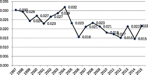
The variance of q^k_i,j,t is used as the index of market integration between regions i and j. First, Figure 1 presents the average index of market integration over 29 regions from 1997 to 2015. It might be divided into two periods, namely phase of disintegration (1997–2003) and phase of integration (2004–2015). In the first phase, the average index of market integration is in the range 0.023–0.030 and is high and less volatile. However, it falls sharply from 2004. After 2004, the highest value is 0.023 in 2008, and the lowest value is 0.016 in 2006. The market integration has appeared in the last a few years. During this period, most regions tend to be integrated, and how market integration evolves between regions needs to be explored.

Figure 1. Average index of market integration in China (1997 − 2015).

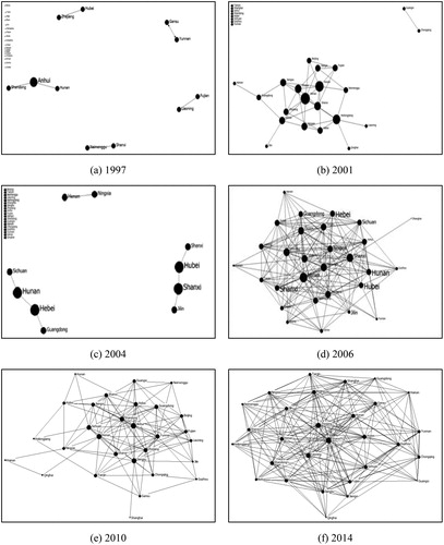
Second, 0.022 is set as the critical value, which is the average value of the market integration index over all 19 years and 29 provinces, to construct cut-off matrices. Network graphs for six years, based on these cut-off matrices, are shown in Figure 2, where nodes represent corresponding provinces, and the existence of a link between a pair of nodes means that the market integration index between them is less than the critical value. It also could be understood as that these two provinces are more integrated than those without links. To be clear, the size of a node is set as associating positively with its degree, represented by deg(z), which is the number of links incident to the node z. Some descriptive statistical indicators of degree appear in Table 2.

Figure 2. Networks of market integration (cut-off value: 0.025).

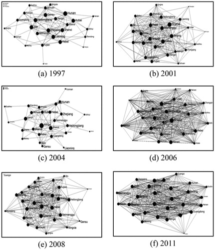
Table 2. Descriptive statistics for degree of individual regions.

	Mean	Std dev.	Sum.	Min.	Max.
1997	5.310	3.333	154	0	11
1998	5.862	3.608	170	0	14
1999	13.586	5.170	394	0	22
2000	8.345	4.801	242	0	18
2001	13.793	5.467	400	2	23
2002	10.069	3.991	292	0	16
2003	9.448	4.832	274	0	18
2004	4.345	2.745	126	0	9
2005	13.586	6.037	394	0	22
2006	25.586	2.895	742	15	28
2007	17.586	6.825	510	0	24
2008	15.655	5.785	454	0	24
2009	16.966	5.505	492	5	24
2010	21.655	4.301	628	12	27
2011	23.448	3.918	680	9	28
2012	25.517	2.724	740	16	28
2013	21.517	4.320	624	14	28
2014	26.138	2.569	758	18	28
2015	23.034	4.037	694	16	28

Source: Authors’ calculation.

From a network perspective, a trend from disintegration to integration appears for the entire domestic market. The trend is clear in Figure 2 and can also be illustrated by Table 2. Table 2 defines the sum of degree as ${\sum }_{z=1}^{29}\mathrm{deg}\left(z\right),$ which can be read as an index of market integration from a macro-perspective. This index is far lower in phase 1 than in phase 2. The mean of this value is 256.50 in phase 1 and 610.55 in phase 2. The maximum in phase 1 is 400 (in 2001), which is close to the minimum in phase 2 (394 in 2005), and the maximum in phase 2 is 758 (in 2014), which is 6.02 times the minimum in phase 1 (126 in 2004).

In addition, the promotion of the integration of the entire domestic market occurs because almost all the regions are involved in the process of market integration in phase 2, which does not occur either within a few parts of China, or in some so-called regional clubs. Even in 2008, most of the regions are connected with others, not to mention that networks in 2012 or 2014 are almost complete.

As for those ‘developed regions’, they contribute more in phase 2 than in phase 1 to DMI. In Figure 2, there exists a core–periphery phenomenon in market integration. However, the core nodes are not the developed regions, such as Shanghai or Guangdong, but those regions that rely more on resources, agriculture or primary processing, such as Shanxi or Heilongjiang. Shanghai is even an isolated node in 1997 and 2004. However, the core–periphery phenomenon in market integration is reversed in phase 2. There are barely differences in the degree of nodes. Most of the regions that have been through sharp increases in degree are developed regions in China, such as Shanghai from 0 to 27, Jiangsu from 2 to 28, Guangdong from 7 to 25, and Beijing from 4 to 25 in the sample period.

To ensure that these conclusions about market integration are robust, 0.020 and 0.015 are set as two other critical values. The network graphs appear in the Appendix. These graphs confirm our present findings. Summarising all the above results, the unification of regional markets in China has been occurring at the national and regional levels since 2004.

5. The dynamic relationship between DMI and regional economic growth

5.1. Estimation results

The level of market integration is visually found to be different in phase 1 (1997–2003) compared with that in phase 2 (2004–2015). But visual inspection can be misleading and hence to confirm (any) dynamic pattern between DMI and regional growth, we estimate spatial econometric β-convergence models. We do this separately for eight sub-periods of eight years, starting with the period 1997–2004, followed by 1998–2005, …., until 2008–2015. Doing so, we find a diverging trend in phase 1 and a trend of convergence in phase 2; that is, every sub-period is divergent, except for the period 2004–2015. For this reason, it is acceptable to set 2004 as the trend-break point within the period 1997–2015. Next, β-convergence models are estimated over the entire period and separately in two different sub-periods: the first ranging from 1997 to 2003 and the second ranging from 2004 to 2015. In addition, the average values of the reciprocal matrices over the corresponding periods have been calculated, and all the reciprocal matrices involved are normalised using row standardisation.

Table 3 displays the estimation results, including the fixed effect model (FE), spatial autocorrelation model with fixed effects (FESAR), and spatial error model with fixed effect (FESEM). Generally, a FE model is particularly appropriate when the regression analysis is limited to a precise set of individuals (regions). All econometric approaches yield qualitatively similar conclusions. The results of FE are benchmarks to be compared with the last two models, so it can be tested whether market integration contributes to regional economic growth and convergence.

Table 3. Estimation results (fixed effect models).

	1997–2015			1997–2003			2004–2015
	(FE)	(FESAR)	(FESEM)	(FE)	(FESAR)	(FESEM)	(FE)	(FESAR)	(FESEM)
β	0.024*** (0.000)	0.008*** (0.000)	0.029*** (0.000)	0.057*** (0.000)	−0.004 (0.311)	−0.007 (0.361)	−0.015** (0.024)	−0.006 (0.327)	−0.009 (0.382)
Rho		0.584*** (0.000)			0.534*** (0.000)			0.537*** (0.000)
Lambda			0.609*** (0.000)			0.533*** (0.000)			0.540*** (0.000)
R^2 overall	0.029	0.137	0.029	0.014	0.092	0.122	0.134	0.101	0.134
Log-likelihood		1027.894	1032.847		629.950	629.810		635.384	636.064

Note: Numbers in parentheses are standard errors, and ^***,**,* indicate that the coefficients are statistically significant at the 1, 5 and 10% levels, respectively.

Source: Authors’ calculation.

First, disparity in regional economies has been through a dynamic process from expansion to narrowing. Although divergence is found over the entire period because β in the first model is positive and statistically significant, convergence is very sharp in phase 2. Second, market integration has exerted a significantly positive impact on regional economic growth. In all the models and periods, rho and lambda are positive and statistically significant. Finally, the relationship between market integration and regional economic growth has changed since 2004. Before then, the higher the level of market integration, the larger the disparity of the regional economy. The differences between the panel data models with market integration and the benchmark models support this conclusion. When the reciprocal matrix is involved in the analysis, the divergence of the regional economy disappears (see the results of FESAR and FESEM in the period 1997–2003) in phase 1. However, the convergence of regional economies disappears (see the results of FESAR and FESEM in 2004–2015).

5.2. Robustness test

Our results may suffer from problems of endogeneity for two reasons. First, market integration and regional economic growth have a mutual influence on each other. Second, there are some omitted variables that are correlated with the index of market integration. Therefore, the spatial lagged variables are correlated with the residuals. To address endogeneity, three measures are adopted.

First, the reciprocal matrix is replaced with a first-order lagged matrix, which means that if the convergence effect is tested in phase 2, the entries in the lagged matrix should be the average values of the reciprocal matrices from 2003 to 2014. It should occur earlier if economic growth has an impact on market integration and the lagged matrix should have a weaker relationship with regional economic growth.

Second, we replaced the reciprocal matrix by its square matrix to reduce the correlation of regional economic growth with market integration. Estimation results with the lagged matrix and the square matrix are displayed in Table 4. From these results, our conclusions are confirmed again.

Table 4. Estimation results with lagged and square of weight matrix.

	2004–2015		1997–2003		2004–2015
	FESAR Lagged W	FESEM Lagged W	FESAR W^2	FESEM W^2	FESAR W^2	FESEM W^2
β	−0.005 (0.326)	−0.008 (0.377)	0.021(0.110)	−0.123 (0.094)	−0.005 (0.313)	−0.008 (0.372)
ρ	0.542*** (0.000)		0.556*** (0.000)		0.564*** (0.000)
Lambda		0.538*** (0.000)		0.879*** (0.000)		0.556*** (0.000)
R^2 overall	0.091	0.127	0.046	0.014	0.093	0.126
Log-likelihood	630.164	630.033	452.225	451.517	630.254	630.141

Note: Numbers in parentheses are standard errors, and ***,** indicate that the coefficients are statistically significant at the 1% and 5% levels, respectively.

Source: Authors’ calculation.

Third, two important control variables, capital and labour, are introduced to avoid endogeneity caused by omitted variables. Therefore, the following two alternative β-convergence models with market integration have been tested: (8) $$\text{ln}\hspace{0.17em}\left(y_{t+m,i}/y_{t,i}\right)={\alpha }_i+\rho {\Sigma }^n{}_j{w}_{i,j}\hspace{0.17em}\text{ln}\hspace{0.17em}\left(y_{t+m,i}/y_{t,i}\right)+\beta \hspace{0.17em}\text{ln}\hspace{0.17em} y_{t,i}+\gamma \hspace{0.17em}\text{ln}\hspace{0.17em}\left(L_{t+m,i}/L_{t,i}\right)+\eta \hspace{0.17em}\text{ln}\hspace{0.17em}\left(K_{t+m,i}/K_{t,i}\right)+{\epsilon }_{t,i}$$(8) and (9) $$\text{ln}\hspace{0.17em}\left(y_{t+m,i}/y_{t,i}\right)={\alpha }_i+\beta \hspace{0.17em}\text{ln}\hspace{0.17em} y_{t,i}+\gamma \hspace{0.17em}\text{ln}\hspace{0.17em}\left(L_{t+m,i}/L_{t,i}\right)+\eta \hspace{0.17em}\text{ln}\hspace{0.17em}\left(K_{t+m,i}/K_{t,i}\right)+{\epsilon }_{t,i,}{\epsilon }_{t,i}=\lambda {\Sigma }^n{}_j{w}_{i,j}{\epsilon }_{t,i}+{\eta }_{t,i}$$(9) where labour (L) is represented with the annual growth rate of the population and capital (K) is represented with the annual growth rate of fixed capital investment. However, there exists the possibility of endogeneity triggered by control variables because labour and capital might move among regions more frequently along with more integrated markets. Therefore, Σn_jw_i,jL_t,i and Σn_jw_i,jK_t,i are used as instrumental variables to execute the regression of the generalised spatial panel two-stage least squares (GS2SLS) and to deal with the additional possibility of endogeneity.

These two models are different from Equations (6)(6) $$\text{ln}\hspace{0.17em}\left(y_{t+m,i}/y_{t,i}\right)={\alpha }_i+\rho {\Sigma }^n{}_j{w}_{i,j}\hspace{0.17em}\text{ln}\hspace{0.17em}\left(y_{t+m,i}/y_{t,i}\right) +\beta \hspace{0.17em}\text{ln}\hspace{0.17em} y_{t,i}+{\epsilon }_{t,}{}_i$$(6) and (7)(7) $$\text{ln}\hspace{0.17em}\left(y_{t+m,i}/y_{t,i}\right)={\alpha }_i+\beta \hspace{0.17em}\text{ln}\hspace{0.17em} y_{t,i}+{\epsilon }_{t,}{}_{i,}{\epsilon }_{t,}{}_i=\lambda {\Sigma }^n{}_j{w}_{i,j}{\epsilon }_{t,}{}_i+{\eta }_{t,i}$$(7) whether in the estimation issues or in the estimation methods. It is more reasonable to test the robustness with them rather than to use them to generate general conclusions. Estimation results appear in Table 5. All the values of R-squared increase significantly compared with Table 3 when two new variables are included in the models. None of the conclusions about the matrix of market integration changes, which implies that the conclusions in Section 4 are robust.

Table 5. Estimation results of GS2SLS.

	1997–2003		2004–2015
	FE	GS2SLS	FE	GS2SLS
β	0.036*** (0.000)	0.021** (0.006)	–0.003 (0.498)	0.026** (0.014)
γ	−1.007*** (0.000)	−0.996*** (0.000)	−0901*** (0.000)	−0.981*** (0.000)
η	0.083*** (0.000)	0.070*** (0.000)	0.041** (0.007)	0.074*** (0.000)
ρ		0.287** (0.015)		2.214** (0.004)
R^2 overall	0.691		0.483
Raw movements R^2		0.994		0.979
Raw movements adjust R^2		0.992		0.980
Log-likelihood		616.973		648.335

Note: Numbers in parentheses are standard errors, and ***,** indicate that the coefficients are statistically significant at the 1% and 5% levels, respectively.

Source: Authors’ calculation.

The estimation results in Table 5 might put forward some interesting questions that are worth addressing in the future. First, compared with Table 3, the divergence trend was more noticeable in phase 1 and the convergence trend disappeared in phase 2. This might mean that accumulation of productive factors was the most important driving force of regional economic growth before 2015, which would have led to convergence due to diminishing marginal returns of labour and capital. The associated possibility is that increasing marginal returns of knowledge and human resources did not play a crucial role in this period. Second, the divergence effects come out when Σn_jw_i,jL_t,i and Σn_jw_i,jK_t,i are used as instrumental variables in phase 2. Considering that convergence turns into divergence after controlling for flows of labour and capital through inter-regional markets, a better choice would be deregulating flows of factors to reduce the regional disparity. Third, gamma is significantly negative while eta is significantly positive. The rationale of this result is that China was still rich in labour and short of capital in this period. In phase 2, gamma increases both in absolute value and significant level when Σn_jw_i,jL_t,i is introduced, which means that labour mobility is an important force to balance the spatial differences in marginal returns of labour. Based on these three points, place-based polices to encourage labour to move out of low productive regions and encourage capital to flow into these regions could reduce the disparity of regional economic growth. This finding is in accord with Greenstone, Hornbeck, and Moretti (2010).

6. Discussion

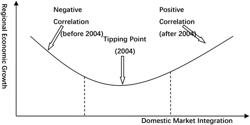
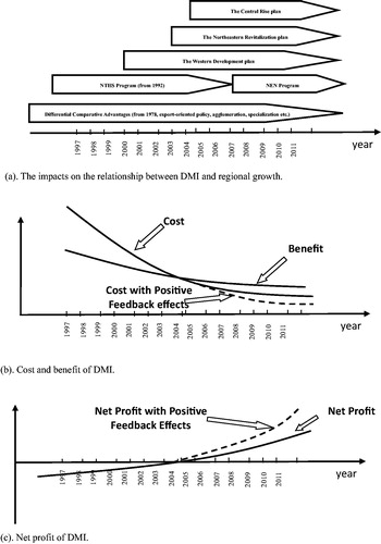
A U-shaped curve to reflect roughly the dynamic relationship between DMI and regional economic growth could be drawn (see Figure 3). Many contributions to economic theory have shown how regional trade can influence economic growth. We highlight three factors which in our reading of China’s economic development have been critical in generating this U-shaped pattern.

Figure 3. The dynamic relationship of DMI and regional economic growth in China.

6.1. The strategy of unbalanced development

The central government defines four regions officially. The eastern, central, and western regions announced in the Seventh Five-Year Plan of China in 1986 and the northeastern region announced in 2002. Each of them includes several provinces. In the early years of the economic reform, the eastern region was given more preferential policies than others to develop an export-oriented economy. As a result, when a modern industrial system was well established in the eastern region, the other regions were still underdeveloped. To narrow the gap, the central government proposed the Western Development Plan in 2000, the Northeastern Revitalisation Plan in 2003 and the Central Rise Plan in 2004. A system of policies and institutions to reduce transaction costs have been established ever since. First, rapid development of financial markets generated lower and lower financing cost. For example, backed by the central government, Sichuan have made a series of policies and development plans to boost financial markets since 2002. Corporate finance by capital market and debt market reached 220.9 billion RMB in 2015, which was an increase of 46% on the previous year. The financing amount in debt markets ranked fourth out of 32 provinces (http://sichuan.scol.com.cn/). Second, reform of administrative systems improved the efficiency of public sectors. For example, the central government has been encouraging local governments to provide E-Government since the 1990s. However, E-Government was not listed on the local governors’ major agenda in less-developed regions before the twenty-first century. Substantial progress happened with the help of the regional development strategies mentioned above. Based on the Annual Report on China’s E-Government Development (2015–2016) (Li & Du, 2016), Sichuan (in the western region), Hunan, and Hubei (in the central region) ranked in the top five out of 32 provinces in 2015. There were also six other provinces from less-developed regions ranked in the first half. As E-Government develops in depth, the efficiency of public sectors continues to improve, which significantly reduces transaction costs of market players. When transaction costs are high, individuals or firms cannot get enough revenue to offset expenses of exchanging factors and goods, or supporting a high level of division of labour and investment. The establishment of appropriate institutions and policies increased market function and stimulated more trade, then economic growth came about. Furthermore, an increasingly large share of public resources has also been invested in these regions to upgrade regional infrastructure, health and social services, education, science and technology.

6.2. Diversity of comparative advantages

In the 1980s, most of the provinces in China had similar comparative advantages (disadvantages) relative to the rest of world, such as low wages for labour, similar industrial structures, low technological levels, and low endowments of human capital. Under these circumstances, as Venables (2003) shows, if they were obliged to trade with each other all areas would lose because the benefit from international trade is more than from domestic trade. Markets would not become more integrated because domestic trade has negative effects on regional economic growth. It was a rational choice for local governments to avoid trading with other domestic regions. Movements towards international integration and trade liberalisation could be considered as factors that possibly favour the emergence of regional economic agglomeration inside countries (Monfort & Nicolini, 2000). At first, some regions had advantages that other regions did not, such as low transportation costs due to location, low costs of production due to the central government’s policies, and so on. Whatever these advantages were, they caused some regions to develop more quickly than others. Resources continued to move into these so-called ‘developed regions’ for a long time. As a result, disparity in the regional economies increased substantially. Opportunities to benefit from DMI are accompanied by the divergence of regional economies because regions form different comparative advantages through the development of a market economy and the long-term export-oriented economy. Market integration is mutually beneficial to both ‘developed regions’ and ‘low-income regions’, especially the latter.

6.3. An efficient transportation system

Enhancement of transportation networks in a country has direct and indirect impacts on the relationship between DMI and regional economic growth. The direct effect is that lower transportation costs make trade that used to be unprofitable happen. The indirect effect is that lower transportation costs can boost the spatial spillover effect by facilitating market access, promoting specialisation and agglomeration (Böventer, 1976), triggering diffusion of knowledge (Mokyr, 2002), and increasing rate of innovation (Grossman & Helpman, 1993).

In 1992, the Chinese State Council approved the construction of the National Trunk Highway System (NTHS) consisting of seven horizontal and five vertical axes (‘7–5’ network). The network, including 41,000 km tolled expressways, was originally planned to be completed by 2020, but was completed ahead of schedule by the end of 2007. At the same time, China also improved 400,000 km of national highways, provincial highways and county roads. The central government and local governments spent about 40 billion dollars each year to make those accomplishments. The objectives of the NTHS programme were to connect all provincial capitals and cities with an urban registered population above 500,000 on a single expressway network.

Given the progress in the construction of the NTHS ahead of plan, the State Council approved an even more ambitious follow-up programme for highway construction in 2004. It is the National Expressway Network (NEN), or so-called ‘7–9–18’ system, which has the stated objective to connect all cities with an urban registered population of more than 200,000, and is planned to be completed by 2020.

6.4. Cost, benefit and the changing relationship

DMI improves regional economic growth when benefits surpass the costs of inter-regional trade. The benefit comes mainly from arbitrage opportunities arising out of a price gap between two regions, which is also the core tenet of the ‘law of one price’. The costs include transaction cost, transportation cost, production cost, etc. The latter would decrease because of a diffusion of knowledge, learning effects and accelerating innovation accompanied by market integration. Figure 4 demonstrates the evolutionary process of cost and benefit of inter-regional trade which could influence the dynamic relationship between DMI and regional economic growth, as Figure 3 shows. Figure 4(a) lists causations of the changing relationship and their timeline. Price gap decreases when two domestic markets tend to be integrated, which generates a benefit curve with negative slope (see Figure 4(b)). The improvement of institutions, the trend of regional policies, the enhancement of transportation infrastructure and the variety of regional economies generate a downward sloping cost curve which is sharper than the benefit curve (see Figure 4(b)). Accordingly, the net profit curve of DMI is upward sloping, as Figure 4(c) shows with a solid line. Since DMI can reduce production costs by triggering the diffusion of knowledge, accelerating the speed of learning and increasing the rate of innovation, the positive feedback effects might be reinforced between DMI and regional economic growth, with specialisation and agglomeration as transmission mechanisms (see the dashed lines in Figure 4(b) and 4(c)).

Figure 4. The evolutionary process of cost and benefit of inter-regional trade.

7. Conclusion

This paper has presented novel empirical findings on the impact of DMI on China’s regional economic growth. We found that the year 2004 represented a tipping point when the impact of greater DMI on regional economic growth changed from being negative to becoming positive. In recent years, the process of market integration has contributed considerably to regional economic growth.

A trend occurs from disintegration towards integration for the entire domestic market. In phase 1, a clear core–periphery pattern exists in DMI. However, the core nodes are not developed regions, but are those regions that rely heavily on resources, agriculture or primary processing. In phase 2, developed regions contribute more than ever to DMI, and the core–periphery pattern almost disappears, accompanied by the level of DMI becoming increasingly large. Almost all regions are involved in the process of market integration in phase 2, which does not occur either within only a few parts or in some so-called regional clubs (unlike what happened during 1997–2004).

A trend of divergence towards convergence exists in regional economic growth in China. The promotion of market integration plays an important role in the process of transformation. In phase 1, there are negative spillover effects between domestic regions that are strengthened by market integration, or economic growth in one region is more harmful to another region if the regions are highly integrated. In phase 2, there are positive spillover effects between domestic regions that are strengthened by market integration, or economic growth in one region is more helpful to another region if they are highly integrated.

An explanation is available for differences between phases 1 and 2. The first condition is the improvement of institutions and policies. The central government proposed the Western Development Plan in 2000, the Northeastern Revitalisation Plan in 2003 and the Central Rise plan in 2004. A system of policies and institutions to reduce transaction costs has been established ever since. The second condition is the variety of comparative advantages. In the early years of reform, all the regions in China had similar comparative advantages (disadvantages) relative to the rest of world. A rational choice occurred to trade with other countries rather than among domestic regions. The coastal areas obtained more benefits from the process of reform and opening because of geographical advantages and preferential policies. As time went on, domestic regions formed different comparative advantages, and DMI became mutually beneficial to both ‘developed regions’ and ‘low-income regions’. The third condition is the accomplishment of the NTHS that can boost spatial spillover effects by facilitating market access, promoting specialisation and agglomeration, triggering diffusion of knowledge, and increasing rate of innovation. These three conditions determine transaction costs, production costs, and transportation costs. They suffice to make the tipping point emerge that the benefit of DMI exceeds the total cost.

This article has focused on the macroscopic state of the relationship between DMI and regional economic growth. Future research can make for a better understanding of related issues by exploring microeconomic evidence. For example, researchers could study the decision-making process of local governors, entrepreneurs and consumers adopting a case-based research orientation to uncover under which conditions local governors are inclined to lower entry barriers or entrepreneurs from different regions tend to trade with each other. Future research should also deepen cognition about how DMI influences regional economic growth as a transmission mechanism. Could DMI amplify the effects of institutions on regional economic growth? Are direct or indirect effects of transportation systems on regional economic growth more significant? Can market power or benefit from the variety of comparative advantages defeat regional protectionism to improve DMI and regional economic growth? To prepare the ground for future studies, our analysis has established that greater market integration has contributed to Chinese regional economic growth, helped by appropriate policies and institutions and efficient transportation systems.

Disclosure statement

No potential conflict of interest was reported by the authors.

Additional information

Funding

This work was supported by National Natural Science Foundation of China [Grant Number 71473059].

Notes

1 https://www.conferenceboard.org/data/economydatabase/index.cfm?id=27762

Appendix

Figures of market integration networks based on alternative critical values

 

Figure A1. Networks of market integration (cut-off value: 0.020).

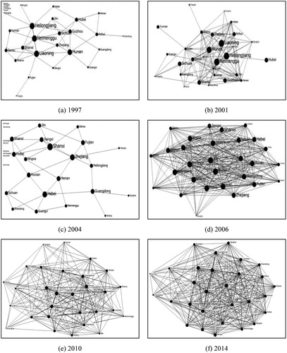
Figure A2. Networks of market integration (cut-off value: 0.015).

References

- Bai, C.-E., Lu, J., & Tao, Z. (2010). Capital or knowhow: The role of foreign multinationals in Sino-foreign joint ventures. China Economic Review, 21(4), 629–638. doi: 10.1016/j.chieco.2010.06.007
- Bai, C.-E., Ma, H., & Pan, W. (2012). Spatial spillover and regional economic growth in China. China Economic Review, 23(4), 982–990. doi: 10.1016/j.chieco.2012.04.016
- Barro, R. J., Sala, I., & Martin, X. (1992). Convergence. Journal of Political Economy, 100(2), 223–251. doi: 10.1086/261816
- Bosworth, B., & Collins, S. M. (2008). Accounting for growth: Comparing China and India. Journal of Economic Perspectives, 22(1), 45–66. doi: 10.1257/jep.22.1.45
- Böventer, E. (1976). Transportation costs, accessibility, and agglomeration economies. Papers in Regional Science, 37(1), 167–183.
- Brun, J.-F., Combes, J.-L., & Renard, M.-F. (2002). Are there spillover effects between coastal and noncoastal regions in China? China Economic Review, 13(2-3), 161–169. doi: 10.1016/S1043-951X(02)00070-6
- Chow, G. C., & Li, K. W. (2002). China’s economic growth: 1952–2010. Economic Development and Cultural Change, 51(1), 247–256. doi: 10.1086/344158
- Greenstone, M., Hornbeck, R., & Moretti, E. (2010). Identifying agglomeration spillovers: Evidence from winners and losers of large plant openings. Journal of Political Economy, 118(3), 536–598.
- Grossman, G. M., & Helpman, E. (1993). Innovation and growth in the global economy (1st ed.). Cambridge, MA: MIT Press.
- Islam, N. (2003). What have we learnt from the convergence debate? Journal of Economic Surveys, 17(3), 309–362. doi: 10.1111/1467-6419.00197
- Ke, S. (2015). Domestic market integration and regional economic growth—China’s recent experience from 1995–2011. World Development, 66, 588–597. doi: 10.1016/j.worlddev.2014.09.024
- LeSage, J., & Pace, R. K. (2010). Introduction to spatial econometrics (1st ed.). Boca Raton, FL: CRC Press.
- Li, H., & Liang, H. (2009). Health, education, and economic growth in China: Empirical findings and implications. China Economic Review, 20(3), 374–387. doi: 10.1016/j.chieco.2008.05.001
- Li, H., Loyalka, P., Rozelle, S., & Wu, B. (2017). Human capital and China’s future growth. Journal of Economic Perspectives, 31(1), 25–48. doi: 10.1257/jep.31.1.25
- Li, J., & Du, P. (2016). Annual report on China’s e-government development (2015-2016). Beijing: Social Sciences Academic Press. (in Chinese)
- Lin, G., Long, Z.-H., & Wu, M. (2006). A spatial investigation of σ-convergence in China. The Journal of Quantitative & Technical Economics, 23(4), 14–21. (in Chinese)
- Lu, M., & Chen, Z. (2006). Government behavior, market integration, and industrial agglomeration in China (1st ed.). Shanghai: Shanghai Remin Publishing Company.
- Lu, M., & Chen, Z. (2009). Increasing return, development strategy and regional economic segmentation. Economic Research Journal, 39, 54–63. (in Chinese)
- Mokyr, J. (2002). The gifts of Athena: Historical origins of the knowledge economy (1st ed.). Princeton, NJ: Princeton University Press. doi: 10.1086/ahr/109.1.136
- Monfort, P., & Nicolini, R. (2000). Regional convergence and international integration. Journal of Urban Economics, 48(2), 286–306. doi: 10.1006/juec.1999.2167
- Parsley, D., & Wei, S.-J. (2001). Explaining the border effect: The role of exchange rate variability, shipping costs, and geography. Journal of International Economics, 55(1), 87–105. doi: 10.1016/S0022-1996(01)00096-4
- Poncet, S. (2003). Domestic market fragmentation and economic growth in China. Jyvsky: The 43rd European Congress of the Regional Science Association.
- Poncet, S. (2005). A fragmented China: Measure and determinants of Chinese domestic market disintegration. Review of International Economics, 13(3), 409–430. doi: 10.1111/j.1467-9396.2005.00514.x
- Qian, Y. (2002). How reform worked in China. Retrieved from https://ssrn.com/abstract=317460
- Samuelson, P. A. (1964). Theoretical notes on trade problems. Review of Economics and Statistics, 46(2), 145–154.
- Scherngell, T., Borowiecki, M., & Hu, Y. (2014). Effects of knowledge capital on total factor productivity in China: A spatial econometric perspective. China Economic Review, 29, 82–94. doi: 10.1016/j.chieco.2014.03.003
- Solow, R. M. (1956). A contribution to the theory of economic growth. Quarterly Journal of Economics, 70(1), 65–94.
- Su, Y., & Liu, Z. (2016). The impact of foreign direct investment and human capital on economic growth: Evidence from Chinese cities. China Economic Review, 37, 97–109. doi: 10.1016/j.chieco.2015.12.007
- Sun, X., Chen, F., & Hewings, G. J. (2017). Spatial perspective on regional growth in China: Evidence from an extended neoclassic growth model. Emerging Markets Finance and Trade, 53(9), 2063–2081. doi: 10.1080/1540496X.2016.1275554
- Tian, L., Wang, H. H., & Chen, Y. (2010). Spatial externalities in China regional economic growth. China Economic Review, 21, S20–S31. doi: 10.1016/j.chieco.2010.05.006
- Venables, A. J. (2003). Winners and losers from regional integration agreements. The Economic Journal, 113(490), 747–761. doi: 10.1111/1468-0297.t01-1-00155
- Wang, Y., & Yao, Y. (2003). Sources of China’s economic growth 1952–1999: Incorporating human capital accumulation. China Economic Review, 14(1), 32–52.
- Woo, W. T. (1999). The real reasons for China’s growth. The China Journal, 41, 115–137. doi: 10.2307/2667589
- Ying, L. G. (2000). Measuring the spillover effects: Some Chinese evidence. Papers in Regional Science, 79(1), 75–89. doi: 10.1007/s101100050004
- Ying, L. G. (2003). Understanding China’s recent growth experience: A spatial econometric perspective. Annals of Regional Science, 37(4), 613–628. doi: 10.1007/s00168-003-0129-x
- Young, A. (2000). The razor’s edge: Distortions and incremental reform in the People’s Republic of China. Quarterly Journal of Economics, 115(4), 1091–1135. doi: 10.1162/003355300555024
- Zhang, Q., & Felmingham, B. (2002). The role of FDI, exports and spillover effects in the regional development of China. Journal of Development Studies, 38(4), 157–178. doi: 10.1080/00220380412331322451