Probability weighting functions obtained from Hong Kong index option market

Abstract

In this paper we estimate the pricing kernel from the Hong Kong index option market and obtain the empirical probability weighting functions based on the rank-dependent expected utility. The empirical pricing kernel is estimated semi-parametrically as the ratio of the risk-neutral and objective densities. We employ a two-step estimation procedure to estimate the objective and risk-neutral densities under a consistent parametric framework of the non-affine generalised autoregressive conditional heteroskedasticity (G.A.R.C.H.) diffusion model. In the first step, we develop a continuous particle filters-based maximum likelihood estimation method to estimate the objective parameters of the G.A.R.C.H. diffusion model using the Hang Seng Index (H.S.I.) returns. In the second step of our estimation, we depart from the usual pure calibration approach and use the H.S.I. option prices to estimate the risk-neutral parameters of the G.A.R.C.H. diffusion model by constraining certain parameters to be consistent with the time-series behaviour of H.S.I. returns. Based on the estimated objective and risk-neutral parameters, the objective and risk-neutral densities are obtained by inverting the corresponding characteristic functions. Empirical results indicate that the empirical pricing kernel estimated from the Hong Kong index option market is non-monotonic and the estimated probability weighting functions are S-shaped, which implies that investors underweight small probability events and overweight large ones.

Keywords:

• Pricing kernel
• probability weighting
• rank-dependent utility
• option prices
• G.A.R.C.H. diffusion model

JEL CLASSIFICATIONS:

• C13
• C32
• C58
• G13

1. Introduction

The behaviour of market investors has always been in focus in the literature on financial economics. Naturally, it involves the pricing kernel (Rosenberg & Engle, 2002) or stochastic discount factor (Cochrane, 2001). In standard economic theory, the pricing kernel is monotonically decreasing in investor wealth or market return and corresponds to a positive risk aversion function. However, there has been a lot of discussion about the reliability of this theory. In the past decade, a large number of empirical studies have provided evidence of a non-monotonically decreasing pricing kernel, which has been referred to as the ‘pricing kernel puzzle’ or ‘risk aversion puzzle’ (Aït-Sahalia & Lo, 2000; Jackwerth, 2000; Rosenberg & Engle, 2002). Beare and Schmidt (2016) and Golubev et al. (2014) provide further empirical evidence of a non-monotonic pricing kernel by conducting formal statistical tests. Using data on an exchange traded fund replicating the S&P 500 index, Figlewski and Malik (2014) also confirm the pricing kernel puzzle. Recently, Cuesdeanu and Jackwerth (2016) use a novel test and forward looking information only to confirm the presence of the pricing kernel puzzle in the S&P 500 index option market.

Many researchers try to explain the pricing kernel puzzle with several approaches, including investors’ heterogeneous beliefs (Detlefsen et al., 2007; Bakshi et al., 2010; Ziegler, 2007), misspecification of the underlying state space (Chabi-Yo, 2012; Chabi-Yo et al., 2008; Christoffersen et al., 2013), ambiguity aversion (Gollier, 2011), investors sentiment (Barone-Adesi et al., 2017), etc. In this paper we consider a pricing kernel based on the rank-dependent expected utility of Quiggin (1993), one of the most important generalisations of expected utility theory, with a probability weighting function. We show that the rank-dependent expected utility with the probability weighting function is able to explain the properties of the empirical pricing kernel estimated from the Hong Kong index option market.

In the last decades, there has been a large amount of literature on the estimation of the pricing kernel. A number of earlier papers estimate the pricing kernel using aggregate consumption data (Chapman, 1997; Hansen & Jagannathan, 1991); problems with imprecise measurement of aggregate consumption can weaken the empirical results of these papers. Thus, many authors have used the option prices to estimate the pricing kernel. This approach avoids the use of aggregate consumption data. Among others, Rosenberg and Engle (2002) emphasise the advantages of option prices over consumption data. Based on the option prices, three types of estimation approaches have been proposed, including the parametric approach (Audrino & Meier, 2012; Rosenberg & Engle, 2002), nonparametric approach (Aït-Sahalia & Lo, 2000; Belomestny et al., 2017; Härdle et al., 2015; Jackwerth, 2000; Song & Xiu, 2016) and semiparametric approach (Chernov, 2003; Detlefsen et al., 2007). In this paper, we follow a semiparametric approach to derive the pricing kernel and construct the implied probability weighting function by estimating the ratio of the risk-neutral and objective densities. The advantage of the semiparametric approach is that it avoids the use of parametric pricing kernel specification, which imposes a strict structure on the kernel so that it too restrictive to account for the dynamics of the risk preference, and bandwidth selection, which influences the shape of the pricing kernel. The semiparametric approach for estimating the pricing kernel is flexible and simple to implement.

Previous econometrics studies are concerned with deriving the empirical pricing kernel by estimating the objective and risk-neutral densities separately, and mainly relying on the discrete-time generalised autoregressive conditional heteroskedasticity (G.A.R.C.H.) model of Bollerslev (1986, 1987) or/and affine stochastic volatility model of Heston (1993). Our estimation procedure is based on the objective and risk-neutral densities and these distributions are derived with a consistent parametric stochastic volatility framework of a non-affine G.A.R.C.H. diffusion model. From these densities we construct the corresponding pricing kernel. The G.A.R.C.H. diffusion model is a non-affine stochastic volatility model, which is a weak limit of discrete-time G.A.R.C.H.(1,1) model and has been found to capture the dynamics of the financial time series much better than the affine Heston stochastic volatility model. A number of recent papers have provided strong evidence for the G.A.R.C.H. diffusion model, not only for returns data but also for options data (Christoffersen et al., 2010; Kaeck & Alexander, 2013; Wu et al., 2012, forthcoming). Thus, the model is well suited for our estimation of the pricing kernel, and hence the probability weighting function.

In this paper, the objective and risk-neutral densities are derived by estimating the objective and risk-neutral parameters of the G.A.R.C.H. diffusion model in a way that maintains the internal consistency of the objective and risk-neutral measures. To achieve this goal, we employ a two-step estimation procedure. In the first step, we develop a continuous particle filters-based maximum likelihood estimation method to estimate the objective parameters of the G.A.R.C.H. diffusion model using the Hong Kong Hang Seng Index (H.S.I.) returns over a long time span. The continuous particle filters-based maximum likelihood estimation method is easy to implement and can be used to estimate the nonlinear models that include unobservable state variables efficiently (Christoffersen et al., 2010; Duan & Fulop, 2009; Malik & Pitt, 2011; Pitt et al., 2014). In the second step of our estimation, we depart from the usual pure calibration approach and use the H.S.I. option prices to estimate the risk-neutral parameters of the G.A.R.C.H. diffusion model by constraining certain parameters to be consistent with the time-series behaviour of H.S.I. returns. More precisely, the volatility of variance and the leverage parameters should be equal under the objective and risk-neutral measures (Broadie et al., 2007). We impose this constraint for both pragmatic and theoretical reasons. First, there is little disagreement in the literature over these parameter values. Second, joint estimation using both option and underlying asset prices is a computationally demanding task. Based on the estimated objective and risk-neutral parameters, the objective and risk-neutral densities can be obtained by inverting the corresponding characteristic functions of the G.A.R.C.H. diffusion model. The pricing kernel is finally obtained as the ratio of the risk-neutral and objective densities.

The probability weighting functions have been studied extensively in the experimental literature over the past decades (Barberis & Huang, 2008; Polkovnichenko, 2005; Prelec, 1998; Shefrin & Statman, 2000; Tversky & Kahneman, 1992). Empirical papers investigating probability weighting functions include Chabi-Yo and Song (2013), Dierkes (2009, 2013), Kliger and Levy (2009), Polkovnichenko and Zhao (2013) and Wang (2017). In these papers, the authors obtain the probability weighting functions mainly from option prices. The main difference between our paper and theirs lies mainly in the use of a consistent parametric framework of the popular non-affine G.A.R.C.H. diffusion model for estimation. To the best of our knowledge, the G.A.R.C.H. diffusion model has not been used to estimate the probability weighting functions. Also, different from previous empirical studies that investigate probability weighting functions mainly focus on the U.S. S&P 500 index option market, this paper aims to investigate the probability weighting functions empirically for the Hong Kong index option market. We estimate the pricing kernel from the H.S.I. options and obtain the empirical probability weighting functions based on the rank-dependent expected utility. We then employ the estimate of the probability weighting functions to examine characteristic of investors’ decision weights in the Hong Kong stock market.

This paper contributes to the existing literature in several ways. First, to ensure consistency between the objective and risk-neutral measures which is crucial for obtaining reasonable results, a two-step estimation procedure for the popular non-affine G.A.R.C.H. diffusion model is developed. Second, the empirical non-monotonic pricing kernel and S-shaped probability weighting functions are obtained from the Hong Kong index option market. Third, it reveals that investors in the Hong Kong stock market underweight small probability events (tail events) and overweight large ones. Finally, the S-shaped probability weighting function with a utility function exhibiting constant relative risk aversion (C.R.R.A.) based on the rand-dependent utility explains the non-monotonicity of the pricing kernel.

The rest of the paper is organised as follows. In Section 2, we describe the theoretical link between the pricing kernel, probability weighting function and risk-neutral and objective densities. In Section 3, we present under the objective measure the G.A.R.C.H. diffusion model and derive the corresponding system under the risk-neutral measure, which serves as the basis for the estimation of the objective and risk-neutral densities. We describe the two-step estimation procedure used to estimate the objective and risk-neutral densities in Section 4. Section 5 discusses the empirical results obtained from the H.S.I. option market, and Section 6 concludes.

2. Pricing kernel and probability weighting function

In this section, we present a theoretical link between the pricing kernel and probability weighting function based on the rank-dependent expected utility. See Polkovnichenko and Zhao (2013) for detailed discussion of the properties of the pricing kernel with probability weighting function.

Consider an index as a proxy for all wealth in the economy, let S_T be the future price of the index, and S_t be the current price of the index. In the absence of arbitrage, there exists one positive random variable $M_{t,T}$ that prices the index (1) $$S_t=E^{\mathbb{P}}\left[M_{t,T}\right(S_T\left)S_T\right|{\mathcal{F}}_t]$$(1) where $E^{\mathbb{P}}[·|{\mathcal{F}}_t]$ is the expectation with respect to the objective measure $\mathbb{P}$ conditional on the information set ${\mathcal{F}}_t$ available at time t, and $M_{t,T}$ is the projection of the pricing kernel into S_T, which has the same pricing implications as the original one (Rosenberg & Engle, 2002).

According to the risk-neutral valuation principal, the price $S_t$ of the index with payoff $S_T$ can be equivalently represented as (2) $$S_t=E^{\mathbb{Q}}\left[e^{-r\tau }{S}_T\right|{\mathcal{F}}_t]$$(2) where $E^{\mathbb{Q}}[·|{\mathcal{F}}_t]$ is the expectation with respect to the risk-neutral measure $\mathbb{Q}$ conditional on the information set ${\mathcal{F}}_t$ available at time t, r is the risk-free interest rate, and $\tau =T-t.$

Assuming that $p_{t,T}(S_T)$ is the objective density (the probability density function under the objective measure $\mathbb{P}$) of $S_T,$ and $q_{t,T}(S_T)$ is the risk-neutral density (the probability density function under the risk-neutral measure $\mathbb{Q}$) of $S_T.$ From Equation (2)(2) $$S_t=E^{\mathbb{Q}}\left[e^{-r\tau }{S}_T\right|{\mathcal{F}}_t]$$(2) , we have (3) $$\begin{array}{c}{S}_t={\int }_{{\mathbb{R}}^{+}}{e}^{-r\tau }x{q}_{t,T}\left(x\right)\mathrm{d}x={\int }_{{\mathbb{R}}^{+}}{e}^{-r\tau }\frac{q_{t,T}\left(x\right)}{p_{t,T}\left(x\right)}x{p}_{t,T}\left(x\right)\mathrm{d}x\\ =E^{\mathbb{P}}\left[e^{-r\tau }\frac{q_{t,T}\left(S_T\right)}{p_{t,T}\left(S_T\right)}{S}_T|{\mathcal{F}}_t\right]\end{array}$$(3)

Comparing Equations (1)(1) $$S_t=E^{\mathbb{P}}\left[M_{t,T}\right(S_T\left)S_T\right|{\mathcal{F}}_t]$$(1) and (3)(3) $$\begin{array}{c}{S}_t={\int }_{{\mathbb{R}}^{+}}{e}^{-r\tau }x{q}_{t,T}\left(x\right)\mathrm{d}x={\int }_{{\mathbb{R}}^{+}}{e}^{-r\tau }\frac{q_{t,T}\left(x\right)}{p_{t,T}\left(x\right)}x{p}_{t,T}\left(x\right)\mathrm{d}x\\ =E^{\mathbb{P}}\left[e^{-r\tau }\frac{q_{t,T}\left(S_T\right)}{p_{t,T}\left(S_T\right)}{S}_T|{\mathcal{F}}_t\right]\end{array}$$(3) , we get (4) $$M_{t,T}\left(S_T\right)=e^{-r\tau }\frac{q_{t,T}\left(S_T\right)}{p_{t,T}\left(S_T\right)}$$(4)

It is obvious from Equation (4)(4) $$M_{t,T}\left(S_T\right)=e^{-r\tau }\frac{q_{t,T}\left(S_T\right)}{p_{t,T}\left(S_T\right)}$$(4) that we can obtain the empirical pricing kernel by estimating the ratio of the risk-neutral and objective densities. Reasonable estimates for the pricing kernel in Equation (4)(4) $$M_{t,T}\left(S_T\right)=e^{-r\tau }\frac{q_{t,T}\left(S_T\right)}{p_{t,T}\left(S_T\right)}$$(4) should be non-increasing in $S_T,$ thereby implying a risk-averse investor. However, many studies document a humpy pricing kernel that it might be increasing in some range of the market returns (Bakshi et al., 2010; Rosenberg & Engle, 2002). Under expected utility theory, it is difficult to understand the reasons for the shape of the pricing kernel. In this paper, we relax the assumption of expected utility theory, and attempt to explain the non-monotonic pricing kernel (or pricing kernel puzzle) under the rank-dependent expected utility of Quiggin (1993), one of the most important extensions of expected utility theory.

Under rank-dependent expected utility, instead of the true cumulative distribution function, $P_{t,T}(S_T),$ the representative investor uses the following distorted one to make an investment decision (5) $${\tilde{P}}_{t,T}\left(S_T\right)=w\left(P_{t,T}\right(S_T\left)\right)$$(5) where $w(·): [ 0,1 ] \to [ 0,1 ]$ is the probability weighting function, satisfies $w(0)=0$ and $w(1)=1.$ Moreover, w is nonlinear, differentiable, continuous, and non-decreasing.

Given the distribution function $P_{t,T},$ the rank-dependent expected utility is calculated as (6) $$U=\int u\left(S_T\right)\mathrm{d}w\left(P_{t,T}\right)=E\left[u\right(S_T\left)z\right(P_{t,T}\left)\right]$$(6) where $z(P_{t,T})=w\prime (P_{t,T}).$

Following Polkovnichenko and Zhao (2013), under the assumption of complete markets, we have (7) $$M_{t,T}\left(S_T\right)=u\prime \left(S_T\right)z\left(P_{t,T}\right)$$(7)

It is obvious from Equation (7)(7) $$M_{t,T}\left(S_T\right)=u\prime \left(S_T\right)z\left(P_{t,T}\right)$$(7) that the pricing kernel $M_{t,T}$ is linked to the derivative of the probability weighting function $z(P_{t,T})=w\prime (P_{t,T})$ via the marginal utility $u\prime (S_T).$

Considering the influence of the initial wealth, we use $R_T\equiv S_T/S_t$ as a proxy for the gross return on the total investor wealth and assume that the initial wealth is one, we can rewrite the Equations (4)(4) $$M_{t,T}\left(S_T\right)=e^{-r\tau }\frac{q_{t,T}\left(S_T\right)}{p_{t,T}\left(S_T\right)}$$(4) and (7)(7) $$M_{t,T}\left(S_T\right)=u\prime \left(S_T\right)z\left(P_{t,T}\right)$$(7) as (8) $$M_{t,T}\left(R_T\right)=e^{-r\tau }\frac{q_{t,T}\left(R_T\right)}{p_{t,T}\left(R_T\right)}$$(8)

and (9) $$M_{t,T}\left(R_T\right)=u\prime \left(R_T\right)z\left(P_{t,T}\right)$$(9) where $p_{t,T}$ and $q_{t,T}$ now are the objective and risk-neutral densities of $R_T,$ and $P_{t,T}$ now is the cumulative distribution function of $R_T$ and $P_{t,T}^{\prime }=p_{t,T}.$

For any given return $R_T^0,$ assume that $P_{t,T}(R_T^0)=P_{t,T}^0,$ according to Equations (8)(8) $$M_{t,T}\left(R_T\right)=e^{-r\tau }\frac{q_{t,T}\left(R_T\right)}{p_{t,T}\left(R_T\right)}$$(8) and (9)(9) $$M_{t,T}\left(R_T\right)=u\prime \left(R_T\right)z\left(P_{t,T}\right)$$(9) , we have (10) $$\begin{array}{c}w\left(P_{t,T}^0\right)={\int }_0^{P_{t,T}^0}z\left(P_{t,T}\right)\mathrm{d}{P}_{t,T}=c{\int }_0^{R_T^0}\frac{M_{t,T}\left(R_T\right)}{u\prime \left(R_T\right)}{p}_{t,T}\left(R_T\right)\mathrm{d}{R}_T\\ =c{e}^{-r\tau }{\int }_0^{R_T^0}\frac{q_{t,T}\left(R_T\right)}{u\prime \left(R_T\right)}\mathrm{d}{R}_T\end{array}$$(10) where $c=e^{r\tau }{\left({\int }_0^{\infty }\frac{q_{t,T}(R_T)}{u\prime (R_T)}\mathrm{d}{R}_T\right)}^{-1}$ is the normalising constant such that $w(1)=1.$

3. The model

We adopt the non-affine G.A.R.C.H. diffusion model to characterise the dynamics of the underlying asset prices (H.S.I.), and form the basis for the estimation of the objective and risk-neutral densities.

In the G.A.R.C.H. diffusion model, the dynamics under the objective measure $\mathbb{P}$ of the underlying asset price, S_t, and the associated variance, V_t, are assumed to be given by (11) $$\mathrm{d}{S}_t=\mu S_t\mathrm{d}t+\sqrt{V_t}{S}_t\mathrm{d}{W}_{1,t}^{\mathbb{P}}$$(11) (12) $$\mathrm{d}{V}_t={\kappa }^{\mathbb{P}}({\theta }^{\mathbb{P}}-V_t)\mathrm{d}t+\sigma V_t\mathrm{d}{W}_{2,t}^{\mathbb{P}}$$(12) where μ is the mean of the underlying asset returns, ${\theta }^{\mathbb{P}}$ is the long-run mean of variance, ${\kappa }^{\mathbb{P}}$ is the mean reversion rate of variance, σ is the volatility of variance, and $W_{1,t}^{\mathbb{P}}$ and $W_{2,t}^{\mathbb{P}}$ are two standard Brownian motions with ${\text{Corr}}_t(\mathrm{d}{W}_{1,t}^{\mathbb{P}},\mathrm{d}{W}_{2,t}^{\mathbb{P}})=\rho .$ The correlation parameter, ρ, is typically found to be negative, which captures the well-known ‘leverage effect’ originated by Black (1976). That is, when asset prices decrease or returns are negative, the firm becomes more risky due to an increase in its debt-equity ratio, leading to an increase in its volatility (see also Christie (1982)).

The G.A.R.C.H. diffusion model in Equations (11)(11) $$\mathrm{d}{S}_t=\mu S_t\mathrm{d}t+\sqrt{V_t}{S}_t\mathrm{d}{W}_{1,t}^{\mathbb{P}}$$(11) and (12)(12) $$\mathrm{d}{V}_t={\kappa }^{\mathbb{P}}({\theta }^{\mathbb{P}}-V_t)\mathrm{d}t+\sigma V_t\mathrm{d}{W}_{2,t}^{\mathbb{P}}$$(12) has attracted a great deal of attention in recent years in the financial econometrics literature. A number of papers have shown that the model can provide realistic volatility dynamics and good option valuation performance (Christoffersen et al., 2010; Kaeck & Alexander, 2013; Wu et al., 2012; Yang & Kanniainen, 2017).

Following Chernov and Ghysels (2000), we assume that the dynamics of the underlying asset prices have the same form under the risk-neutral measure $\mathbb{Q}$ as under the objective measure $\mathbb{P},$ and the dynamics of (S_t, V_t) under the risk-neutral measure $\mathbb{Q}$ are of the form (13) $$\mathrm{d}{S}_t=r{S}_t\mathrm{d}t+\sqrt{V_t}{S}_t\mathrm{d}{W}_{1,t}^{\mathbb{Q}}$$(13) (14) $$\mathrm{d}{V}_t={\kappa }^{\mathbb{Q}}({\theta }^{\mathbb{Q}}-V_t)\mathrm{d}t+\sigma V_t\mathrm{d}{W}_{2,t}^{\mathbb{Q}}$$(14) where r is the risk-free interest rate, $W_{1,t}^{\mathbb{Q}}$ and $W_{2,t}^{\mathbb{Q}}$ are two standard Brownian motions under the risk-neutral measure with ${\text{Corr}}_t(\mathrm{d}{W}_{1,t}^{\mathbb{Q}},\mathrm{d}{W}_{2,t}^{\mathbb{Q}})=\rho .$ As prior studies constrain ${\kappa }^{\mathbb{Q}}{\theta }^{\mathbb{Q}}={\kappa }^{\mathbb{P}}{\theta }^{\mathbb{P}},$ here we specify a more flexible risk-neutral dynamics in that we allow ${\kappa }^{\mathbb{Q}}{\theta }^{\mathbb{Q}}\ne {\kappa }^{\mathbb{P}}{\theta }^{\mathbb{P}},$ which implies a more flexible variance risk premium (15) $$\lambda \left(V_t\right)={\kappa }^{\mathbb{P}}{\theta }^{\mathbb{P}}-{\kappa }^{\mathbb{Q}}{\theta }^{\mathbb{Q}}+({\kappa }^{\mathbb{Q}}-{\kappa }^{\mathbb{P}})V_t$$(15) that enhances the model flexibility to fit the market option prices.

According to Wu et al. (2012), the characteristic function for the log price $X_T=\hspace{0.17em}\text{log}\hspace{0.17em}{S}_T$ under the objective measure $\mathbb{P}$ is given by (16) $$f_{t,T}^{\mathbb{P}}(X_t,V_t,\tau ;\varphi )=e^{C(\tau ;\varphi )+D(\tau ;\varphi )V_t+\mathbf{i}\varphi X_t}$$(16) where $$\begin{array}{c}C(\tau ;\varphi )=\mathbf{i}\varphi \mu \tau -\frac{1}{2{\sigma }^2{\theta }^{\mathbb{P}}}\left[{\kappa }^{\mathbb{P}}{\theta }^{\mathbb{P}}-\frac{1}{2}\rho \sigma \mathbf{i}\varphi {\left({\theta }^{\mathbb{P}}\right)}^{3/2}\right]\\ \times \left[2\hspace{0.17em}\text{log}\hspace{0.17em}\left(\frac{2d-(d-g)(1-e^{-d\tau })}{2d}\right)+(d-g)\tau \right]\\ +\frac{1}{2}{\sigma }^2{\left({\theta }^{\mathbb{P}}\right)}^2[\frac{16g{\zeta }^2}{{(d^2-g^2)}^2}\text{log}\hspace{0.17em}\frac{2d-(d-g)(1-e^{-d\tau })}{2d}\\ -\frac{4\tau {\zeta }^2(d^2-g^2)+4\tau {\zeta }^2{(d-g)}^2{e}^{-d\tau }-8{\zeta }^2(d+g)(1-e^{-d\tau })}{{(d+g)}^2(d-g)[2d-(d-g\left)\right(1-e^{-d\tau }\left)\right]}]\\ D(\tau ;\varphi )=\frac{2\zeta (1-e^{-d\tau })}{2d-(d-g)(1-e^{-d\tau })}\end{array}$$

and $$\begin{array}{c}\zeta =\frac{1}{2}\mathbf{i}\varphi (\mathbf{i}\varphi -1)\\ d=\sqrt{g^2-4{\sigma }^2\zeta {\theta }^{\mathbb{P}}}\\ g={\kappa }^{\mathbb{P}}-\frac{3}{2}\rho \sigma \mathbf{i}\varphi {\left({\theta }^{\mathbb{P}}\right)}^{1/2}\end{array}$$

The characteristic function for X_T under the risk-neutral measure $\mathbb{Q}$ denoted by $f_{t,T}^{\mathbb{Q}}$ is analogous to the objective characteristic function $f_{t,T}^{\mathbb{P}},$ which can be obtained by replacing the objective parameters in Equation (16)(16) $$f_{t,T}^{\mathbb{P}}(X_t,V_t,\tau ;\varphi )=e^{C(\tau ;\varphi )+D(\tau ;\varphi )V_t+\mathbf{i}\varphi X_t}$$(16) , μ, ${\kappa }^{\mathbb{P}}$ and ${\theta }^{\mathbb{P}},$ with the risk-neutral parameters, r, ${\kappa }^{\mathbb{Q}}$ and ${\theta }^{\mathbb{Q}}.$

Then the objective and risk-neutral densities for $R_T=S_T/S_t$ can be obtained by inverting the characteristic functions $f_{t,T}^{\mathbb{P}}$ and $f_{t,T}^{\mathbb{Q}},$ respectively. Specifically, we have (17) $$p_{t,T}\left(R_T\right)=\frac{1}{R_T}{\widehat{p}}_{t,T}(\hspace{0.17em}\text{log}\hspace{0.17em}{R}_T+\hspace{0.17em}\text{log}\hspace{0.17em}{S}_t)$$(17) (18) $$q_{t,T}\left(R_T\right)=\frac{1}{R_T}{\widehat{q}}_{t,T}(\hspace{0.17em}\text{log}\hspace{0.17em}{R}_T+\hspace{0.17em}\text{log}\hspace{0.17em}{S}_t)$$(18) where (19) $${\widehat{p}}_{t,T}\left(X_T\right)=\frac{1}{2\pi }{\int }_{\mathbb{R}}{e}^{-\mathbf{i}\varphi X_T}{f}_{t,T}^{\mathbb{P}}(X_t,V_t,\tau ;\varphi )\mathrm{d}\varphi$$(19) (20) $${\widehat{q}}_{t,T}\left(X_T\right)=\frac{1}{2\pi }{\int }_{\mathbb{R}}{e}^{-\mathbf{i}\varphi X_T}{f}_{t,T}^{\mathbb{Q}}(X_t,V_t,\tau ;\varphi )\mathrm{d}\varphi$$(20)

The integrals in Equations (19)(19) $${\widehat{p}}_{t,T}\left(X_T\right)=\frac{1}{2\pi }{\int }_{\mathbb{R}}{e}^{-\mathbf{i}\varphi X_T}{f}_{t,T}^{\mathbb{P}}(X_t,V_t,\tau ;\varphi )\mathrm{d}\varphi$$(19) and (20)(20) $${\widehat{q}}_{t,T}\left(X_T\right)=\frac{1}{2\pi }{\int }_{\mathbb{R}}{e}^{-\mathbf{i}\varphi X_T}{f}_{t,T}^{\mathbb{Q}}(X_t,V_t,\tau ;\varphi )\mathrm{d}\varphi$$(20) can be easily computed by using some numerical methods.

Based on the theoretical links between the pricing kernel, probability weighting function and objective and risk-neutral densities in Equations (8)(8) $$M_{t,T}\left(R_T\right)=e^{-r\tau }\frac{q_{t,T}\left(R_T\right)}{p_{t,T}\left(R_T\right)}$$(8) and (10)(10) $$\begin{array}{c}w\left(P_{t,T}^0\right)={\int }_0^{P_{t,T}^0}z\left(P_{t,T}\right)\mathrm{d}{P}_{t,T}=c{\int }_0^{R_T^0}\frac{M_{t,T}\left(R_T\right)}{u\prime \left(R_T\right)}{p}_{t,T}\left(R_T\right)\mathrm{d}{R}_T\\ =c{e}^{-r\tau }{\int }_0^{R_T^0}\frac{q_{t,T}\left(R_T\right)}{u\prime \left(R_T\right)}\mathrm{d}{R}_T\end{array}$$(10) , the pricing kernel and probability weighting function can finally be obtained.

4. Estimation methodology

For computing the objective and risk-neutral densities by Equations (17)(17) $$p_{t,T}\left(R_T\right)=\frac{1}{R_T}{\widehat{p}}_{t,T}(\hspace{0.17em}\text{log}\hspace{0.17em}{R}_T+\hspace{0.17em}\text{log}\hspace{0.17em}{S}_t)$$(17) and (18)(18) $$q_{t,T}\left(R_T\right)=\frac{1}{R_T}{\widehat{q}}_{t,T}(\hspace{0.17em}\text{log}\hspace{0.17em}{R}_T+\hspace{0.17em}\text{log}\hspace{0.17em}{S}_t)$$(18) , we still need to estimate the objective and risk-neutral parameters of the G.A.R.C.H. diffusion model. In this section, we describe how to estimate the objective and risk-neutral parameters of the G.A.R.C.H. diffusion model in a way that maintains the internal consistency of the objective and risk-neutral measures. We employ a two-step estimation procedure.

First, we take the stabilising transformation $X_t=\hspace{0.17em}\text{log}\hspace{0.17em}{S}_t,h_t=\hspace{0.17em}\text{log}\hspace{0.17em}{V}_t.$ By Itô’s lemma, we have (21) $$\mathrm{d}{X}_t=(\mu -\frac{1}{2}{e}^{h_t})\mathrm{d}t+e^{h_t/2}\mathrm{d}{W}_{1,t}^{\mathbb{P}}$$(21) (22) $$\mathrm{d}{h}_t=({\kappa }^{\mathbb{P}}{\theta }^{\mathbb{P}}{e}^{-h_t}-{\kappa }^{\mathbb{P}}-\frac{1}{2}{\sigma }^2)\mathrm{d}t+\sigma \mathrm{d}{W}_{2,t}^{\mathbb{P}}$$(22)

In the empirical literature, the above continuous-time model must be discretised to facilitate the parameter estimation. A simple Euler discretisation leads to the following discrete-time stochastic processes (23) $$y_t=(\mu -\frac{1}{2}{e}^{h_t})\Delta t+e^{h_t/2}\sqrt{\Delta t}{\epsilon }_t$$(23) (24) $$h_t=h_{t-1}+({\kappa }^{\mathbb{P}}{\theta }^{\mathbb{P}}{e}^{-h_{t-1}}-{\kappa }^{\mathbb{P}}-\frac{1}{2}{\sigma }^2)\Delta t+\sigma \sqrt{\Delta t}{\eta }_t$$(24) where $y_t=X_t-X_{t-1}$ is the log return of underlying asset, $\Delta t$ is the time interval,¹ and ${\epsilon }_t=(W_{1,t}^{\mathbb{P}}-W_{1,t-1}^{\mathbb{P}})/\sqrt{\Delta t},{\eta }_t=(W_{2,t}^{\mathbb{P}}-W_{2,t-1}^{\mathbb{P}})/\sqrt{\Delta t}.$ It can be shown that ${\epsilon }_t$ and η_t are independent and identically distributed (i.i.d.) standard normal random variables with ${\text{Corr}}_t({\epsilon }_t,{\eta }_t)=\rho .$

It can be seen that Equations (23)(23) $$y_t=(\mu -\frac{1}{2}{e}^{h_t})\Delta t+e^{h_t/2}\sqrt{\Delta t}{\epsilon }_t$$(23) and (24)(24) $$h_t=h_{t-1}+({\kappa }^{\mathbb{P}}{\theta }^{\mathbb{P}}{e}^{-h_{t-1}}-{\kappa }^{\mathbb{P}}-\frac{1}{2}{\sigma }^2)\Delta t+\sigma \sqrt{\Delta t}{\eta }_t$$(24) constitute a nonlinear and non-Gaussian state-space model that cannot be estimated using the standard Kalman filter. To overcome this problem, we adopt the continuous particle filters-based maximum likelihood estimation method to estimate the model parameters (objective parameters). The log likelihood of the model is given by (25) $$\text{log}\hspace{0.17em}L\left({\Theta }^{\mathbb{P}}\right)=\hspace{0.17em}\text{log}\hspace{0.17em}p(y_1,\dots ,y_T|{\Theta }^{\mathbb{P}})=\sum _{t=0}^{T-1}\hspace{0.17em}\text{log}\hspace{0.17em}p(y_{t+1}|{\mathcal{F}}_t;{\Theta }^{\mathbb{P}})$$(25) via prediction decomposition, where ${\Theta }^{\mathbb{P}}=(\mu ,{\kappa }^{\mathbb{P}},{\theta }^{\mathbb{P}},\sigma ,\rho )\prime$ are the objective parameters of the G.A.R.C.H. diffusion model. In the above equation, the predictive density (likelihood) $p(y_{t+1}|{\mathcal{F}}_t;{\Theta }^{\mathbb{P}})$ can be written as (26) $$p\left(y_{t+1}\right|{\mathcal{F}}_t;{\Theta }^{\mathbb{P}})=\int p(y_{t+1}|h_{t+1};{\Theta }^{\mathbb{P}})p\left(h_{t+1}\right|{\mathcal{F}}_t;{\Theta }^{\mathbb{P}})\mathrm{d}{h}_{t+1}$$(26)

The expression in Equation (26)(26) $$p\left(y_{t+1}\right|{\mathcal{F}}_t;{\Theta }^{\mathbb{P}})=\int p(y_{t+1}|h_{t+1};{\Theta }^{\mathbb{P}})p\left(h_{t+1}\right|{\mathcal{F}}_t;{\Theta }^{\mathbb{P}})\mathrm{d}{h}_{t+1}$$(26) is crucial for the maximum likelihood estimation via particle filters. In fact, the predictive density $p(y_{t+1}|{\mathcal{F}}_t;{\Theta }^{\mathbb{P}})$ can be approximated by using Monte Carlo method, that is, (27) $$\widehat{p}\left(y_{t+1}\right|{\mathcal{F}}_t;{\Theta }^{\mathbb{P}})=\frac{1}{N}\sum _{i=1}^{N}p(y_{t+1}|h_{t+1}^i;{\Theta }^{\mathbb{P}})$$(27) where $h_{t+1}^i, i=1,\dots ,N,$ sampled from the predictive density $p(h_{t+1}|{\mathcal{F}}_t;{\Theta }^{\mathbb{P}})$ via particle filters, which is a sequential Monte Carlo technique using simulated samples to represent prediction and filtering distributions. Updating from the prediction distribution to the filtering distribution is carried out by using the Bayesian rule. Specifically, we have (28) $$\begin{array}{c}p\left(h_{t+1}\right|{\mathcal{F}}_{t+1};{\Theta }^{\mathbb{P}})\propto p(y_{t+1}|h_{t+1};{\Theta }^{\mathbb{P}})p\left(h_{t+1}\right|{\mathcal{F}}_t;{\Theta }^{\mathbb{P}})\\ =p\left(y_{t+1}\right|h_{t+1};{\Theta }^{\mathbb{P}}\left)\int p\right(h_{t+1}|h_t;{\Theta }^{\mathbb{P}})p\left(h_t\right|{\mathcal{F}}_t;{\Theta }^{\mathbb{P}})\mathrm{d}{h}_t\end{array}$$(28) where $p(h_{t+1}|{\mathcal{F}}_{t+1};{\Theta }^{\mathbb{P}})$ is the filtering density. The principle of Bayesian updating implies that the density of the state conditional on all available information can be constructed by combining a prior with a likelihood, recursive implementation of which forms the basis for particle filtering. The particle filtering algorithm thus propagates and updates the samples or ‘particles’ via Equation (28)(28) $$\begin{array}{c}p\left(h_{t+1}\right|{\mathcal{F}}_{t+1};{\Theta }^{\mathbb{P}})\propto p(y_{t+1}|h_{t+1};{\Theta }^{\mathbb{P}})p\left(h_{t+1}\right|{\mathcal{F}}_t;{\Theta }^{\mathbb{P}})\\ =p\left(y_{t+1}\right|h_{t+1};{\Theta }^{\mathbb{P}}\left)\int p\right(h_{t+1}|h_t;{\Theta }^{\mathbb{P}})p\left(h_t\right|{\mathcal{F}}_t;{\Theta }^{\mathbb{P}})\mathrm{d}{h}_t\end{array}$$(28) , which can be approximated by (29) $$\widehat{p}\left(h_{t+1}\right|{\mathcal{F}}_{t+1};{\Theta }^{\mathbb{P}})\propto p(y_{t+1}|h_{t+1};{\Theta }^{\mathbb{P}})\frac{1}{N}\sum _{t=1}^{N}p\left(h_{t+1}\right|h_t^i;{\Theta }^{\mathbb{P}})$$(29) where $h_t^i, i=1,\dots ,N,$ are the equally weighted samples or ’particles’ from the density $p(h_t|{\mathcal{F}}_t;{\Theta }^{\mathbb{P}}).$

In order to sample from the density of Equation (29)(29) $$\widehat{p}\left(h_{t+1}\right|{\mathcal{F}}_{t+1};{\Theta }^{\mathbb{P}})\propto p(y_{t+1}|h_{t+1};{\Theta }^{\mathbb{P}})\frac{1}{N}\sum _{t=1}^{N}p\left(h_{t+1}\right|h_t^i;{\Theta }^{\mathbb{P}})$$(29) , we use the sampling importance resampling (S.I.R.) algorithm of Gordon et al. (1993). However, the resampling step in the standard S.I.R. algorithm creates discontinuity in the likelihood function that is not conducive to numerical optimisation and statistical inference, and makes estimation by maximum likelihood problematic. To overcome this problem, we adopt the continuous S.I.R. (C.S.I.R.) scheme proposed by Malik and Pitt (2011) to compute the likelihood function and conduct the maximum likelihood estimation.

The C.S.I.R. algorithm is outlined below:

Given samples from $h_t^i\sim p(h_t|{\mathcal{F}}_t;{\Theta }^{\mathbb{P}}),i=1,\dots ,N.$

1. Sample ${\tilde{h}}_{t+1}^i\sim p(h_{t+1}|h_t^i;{\Theta }^{\mathbb{P}}),i=1,\dots ,N,$ using Equation (24)(24) $$h_t=h_{t-1}+({\kappa }^{\mathbb{P}}{\theta }^{\mathbb{P}}{e}^{-h_{t-1}}-{\kappa }^{\mathbb{P}}-\frac{1}{2}{\sigma }^2)\Delta t+\sigma \sqrt{\Delta t}{\eta }_t$$(24) .

2. Calculate normalised weights, (30) $${\pi }_{t+1}^i=\frac{{\omega }_{t+1}^i}{\sum _{i=1}^N{\omega }_{t+1}^i},\hspace{1em}i=1,\dots ,N$$(30) where $$\begin{array}{c}{\omega }_{t+1}^i=p\left(y_{t+1}\right|{\tilde{h}}_{t+1}^i;{\Theta }^{\mathbb{P}})\\ ={\left\{2\pi \hspace{0.17em}\text{exp}\hspace{0.17em}\left({\tilde{h}}_{t+1}^i\right)\Delta t\right\}}^{-1/2}\\ \times \hspace{0.17em}\text{exp}\hspace{0.17em}\left\{-\frac{1}{2}{\left[y_{t+1}-\left(\mu -\frac{1}{2}\text{exp}\hspace{0.17em}\left({\tilde{h}}_{t+1}^i\right)\right)\Delta t\right]}^2/(\hspace{0.17em}\text{exp}\hspace{0.17em}({\tilde{h}}_{t+1}^i)\Delta t)\right\}\end{array}$$

3. Resample from a continuous empirical distribution implied by the set of $\{({\tilde{h}}_{t+1}^i,{\pi }_{t+1}^i)|i\in \{1,\dots ,N\}\}$ to obtain the equally weighted filtering samples $h_{t+1}^i\sim p(h_{t+1}|{\mathcal{F}}_{t+1};\Theta ),i=1,\dots ,N$ (For details see Appendix A).

Based on the above C.S.I.R. algorithm, the prediction likelihood may be estimated as (31) $$\widehat{p}\left(y_{t+1}\right|{\mathcal{F}}_t;{\Theta }^{\mathbb{P}})=\frac{1}{N}\sum _{i=1}^{N}p(y_{t+1}|{\tilde{h}}_{t+1}^i;{\Theta }^{\mathbb{P}})=\frac{1}{N}\sum _{i=1}^N{\omega }_{t+1}^i$$(31) where ${\omega }_{t+1}^i,i=1,\dots ,N,$ are simply the unnormalised weights calculated in Step 2 of C.S.I.R. algorithm. The resulting likelihood function in Equation (31)(31) $$\widehat{p}\left(y_{t+1}\right|{\mathcal{F}}_t;{\Theta }^{\mathbb{P}})=\frac{1}{N}\sum _{i=1}^{N}p(y_{t+1}|{\tilde{h}}_{t+1}^i;{\Theta }^{\mathbb{P}})=\frac{1}{N}\sum _{i=1}^N{\omega }_{t+1}^i$$(31) is a smooth function of parameters. Then, the log likelihood can be estimated by (32) $$\text{log}\hspace{0.17em}\widehat{L}\left({\Theta }^{\mathbb{P}}\right)=\sum _{t=0}^{T-1}\hspace{0.17em}\text{log}\hspace{0.17em}\widehat{p}\left(y_{t+1}\right|{\mathcal{F}}_t;{\Theta }^{\mathbb{P}})=\sum _{t=0}^{T-1}\hspace{0.17em}\text{log}\hspace{0.17em}\left(\frac{1}{N}\sum _{i=1}^N{\omega }_{t+1}^i\right)$$(32)

Note that the log likelihood in Equation (32)(32) $$\text{log}\hspace{0.17em}\widehat{L}\left({\Theta }^{\mathbb{P}}\right)=\sum _{t=0}^{T-1}\hspace{0.17em}\text{log}\hspace{0.17em}\widehat{p}\left(y_{t+1}\right|{\mathcal{F}}_t;{\Theta }^{\mathbb{P}})=\sum _{t=0}^{T-1}\hspace{0.17em}\text{log}\hspace{0.17em}\left(\frac{1}{N}\sum _{i=1}^N{\omega }_{t+1}^i\right)$$(32) will not be unbiased. According to Malik and Pitt (2011), we may correct the original (biased) log likelihood as unbiased one by (33) $$\text{log}\hspace{0.17em}\tilde{L}\left({\Theta }^{\mathbb{P}}\right)=\sum _{t=0}^{T-1}\left(\hspace{0.17em}\text{log}\hspace{0.17em}{\mu }_{{\omega }_{t+1}}+\frac{1}{2}\frac{{\sigma }_{{\omega }_{t+1}}^2}{N{\mu }_{{\omega }_{t+1}}^2}\right)$$(33) where $${\mu }_{{\omega }_{t+1}}=\frac{1}{N}\sum _{i=1}^N{\omega }_{t+1}^i,\hspace{1em}{\sigma }_{{\omega }_{t+1}}^2=\frac{1}{N-1}\sum _{i=1}^N{({\omega }_{t+1}^i-{\mu }_{{\omega }_{t+1}})}^2$$

Given the log likelihood approximation $\text{log}\hspace{0.17em}\tilde{L},$ the maximum likelihood estimates of the model parameters (objective parameters) can be obtained by (34) $${\widehat{\Theta }}^{\mathbb{P}}=\text{arg}\underset{{\Theta }^{\mathbb{P}}}{\max }\hspace{0.17em}\text{log}\hspace{0.17em}\tilde{L}\left({\Theta }^{\mathbb{P}}\right)$$(34)

Based on the above estimated parameters, the spot variances can be obtained using the C.S.I.R. filtering algorithm.

Next, we turn to the estimation of risk-neutral parameters ${\Theta }^{\mathbb{Q}}=({\kappa }^{\mathbb{Q}},{\theta }^{\mathbb{Q}},\sigma ,\rho )\prime .$ We impose consistency between the objective and risk-neutral measures in estimation. Specifically, we let the volatility of variance, σ, and the leverage parameters, ρ, be equal under the objective and risk-neutral measures. As the parameters σ and ρ have been estimated in the first step of our estimation, there are only two remaining risk-neutral parameters (${\kappa }^{\mathbb{Q}}$ and ${\theta }^{\mathbb{Q}}$) need to be estimated in the second step of estimation. We optimise over ${\kappa }^{\mathbb{Q}}$ and ${\theta }^{\mathbb{Q}}$ to fit the observed option prices. Specifically, to obtain the estimates of the parameters ${\kappa }^{\mathbb{Q}}$ and ${\theta }^{\mathbb{Q}},$ we minimise squared differences of model and market option prices, that is, (35) $$({\widehat{\kappa }}^{\mathbb{Q}},{\widehat{\theta }}^{\mathbb{Q}})=\text{arg}\min \sum _{j=1}^M(C_j-C_j({\Theta }^{\mathbb{Q}}){)}^2$$(35) where M is the number of option contracts, C_j is the market option price of contract j, and $C_j({\Theta }^{\mathbb{Q}})$ is the corresponding model option price which can be calculated by using the fast Fourier transform approach based on the risk-neutral characteristic function of the G.A.R.C.H. diffusion model (Carr & Madan, 1999).

5. Empirical results

In contrast to many previous studies that have focused mainly on the S&P 500 index option market, we investigate in this paper the empirical pricing kernel and probability weighting functions by focusing on the H.S.I. option market. The H.S.I. serves as an approximation to the Hong Kong economy, and it can be used as a proxy for market portfolio.

5.1. The data

We use daily H.S.I. returns to estimate the objective G.A.R.C.H. diffusion model and to compute the objective density. The sample period is from 4 January 2000 to 4 October 2017, which is chosen to achieve a long sample. The sample size is 4379 for the index returns. The time-series and Q–Q plots of the H.S.I. returns are presented in Figure 1. We can observe from Figure 1(a) that the H.S.I. returns exhibit time-varying volatility and volatility clustering during the sample period. Summary statistics for the H.S.I. returns are shown in Table 1. It can be seen that the H.S.I. returns are skewed and leptokurtic. Jarque–Bera statistics suggests that the assumption of normality is rejected for the H.S.I. return series, which also can be confirmed from the Q–Q plot of the index returns in Figure 1(b). The results suggest the stochastic volatility model, such as the G.A.R.C.H. diffusion model, may be appropriate for modelling the dynamics of the H.S.I.

Table 1. Summary statistics of the H.S.I. returns.

Min	Max	Mean	Std.	Skew	Kurt	Jarque–Bera
−0.1358	0.1341	0.0001	0.0149	−0.0925	11.0866	11937.6746
						(0.000)

Notes: The number in parenthesis is the p-value of Jarque–Bera tests.

Source: Own calculation.

To estimate the risk-neutral parameters of the G.A.R.C.H. diffusion model, we use the H.S.I. option data which is presented in Table 2. The option data are selected as the most actively traded option contracts with maturity about one month on 4 October 2017. Finally, we use the annualised the 1-month Hong Kong Interbank Offer Rate as a proxy for the risk-free interest rate. All of the data are obtained from the Wind Database of China.

Table 2. Selected H.S.I. option data on 4 October 2017.

Option type	Option price	Maturity date	Strike price
Call	568.00	10/30/2017	28000
Call	443.00	10/30/2017	28200
Call	329.00	10/30/2017	28400
Call	241.00	10/30/2017	28600
Call	170.00	10/30/2017	28800
Call	119.00	10/30/2017	29000
Call	80.00	10/30/2017	29200
Call	53.00	10/30/2017	29400
Call	34.00	10/30/2017	29600
Call	22.00	10/30/2017	29800
Call	13.00	10/30/2017	30000
Call	4.00	10/30/2017	30400
Put	2.00	10/30/2017	24800
Put	3.00	10/30/2017	25000
Put	4.00	10/30/2017	25200
Put	5.00	10/30/2017	25400
Put	7.00	10/30/2017	25600
Put	10.00	10/30/2017	25800
Put	13.00	10/30/2017	26000
Put	18.00	10/30/2017	26200
Put	24.00	10/30/2017	26400
Put	32.00	10/30/2017	26600
Put	44.00	10/30/2017	26800
Put	59.00	10/30/2017	27000
Put	79.00	10/30/2017	27200
Put	102.00	10/30/2017	27400
Put	133.00	10/30/2017	27600
Put	176.00	10/30/2017	27800
Put	230.00	10/30/2017	28000
Put	301.00	10/30/2017	28200
Put	393.00	10/30/2017	28400
Put	500.00	10/30/2017	28600

Source: Wind Database of China.

5.2. Estimation results

Based upon the data on the H.S.I. returns, the objective parameters of the G.A.R.C.H. diffusion model can be estimated by adopting the C.S.I.R.-based maximum likelihood estimation method described in Section 4. Table 3 reports the estimation results. Our results show that, under the objective measure, the long-run mean of the variance is ${\theta }^{\mathbb{P}}=0.0522,$ with a mean-reversion speed of ${\kappa }^{\mathbb{P}}=2.3044.$ The estimate of the ‘leverage effect’ parameter ρ is significantly negative, indicating that the return and the variance processes are negatively correlated during the sample period, a well-known empirical fact.

Table 3. Estimation results.

	μ	${\kappa }^{\mathbb{P}}$	${\theta }^{\mathbb{P}}$	σ	ρ	Log-lik
Objective parameters	0.0805	2.3044	0.0522	2.1633	−0.5717	13088.2001
	(0.0407)	(0.7855)	(0.0126)	(0.1532)	(0.0445)
		${\kappa }^{\mathbb{Q}}$	${\theta }^{\mathbb{Q}}$			R.R.M.S.E.
Risk-neutral parameters		0.1990	0.0180			0.3106

Note: The number of particles used in the C.S.I.R.-based maximum likelihood estimation is 500. The number in parenthesis is the standard error. Log-lik denotes the log-likelihood value. R.R.M.S.E. denotes the relative root mean square error.

Source: Own calculation.

Based on the estimated (objective) parameters of the G.A.R.C.H. diffusion model, the spot variances can be estimated via the C.S.I.R. filtering algorithm. Figure 2 shows the filtered variances. Specially, the spot variance on 4 October 2017 is 0.0185.

Using the H.S.I. option data in Table 2, the risk-neutral parameters of the G.A.R.C.H. diffusion model can be estimated. The estimates are reported in Table 3. It can be seen from the table that, under the risk-neutral measure, the long-run mean of the variance is ${\theta }^{\mathbb{Q}}=0.0180,$ with a mean-reversion speed of ${\kappa }^{\mathbb{Q}}=0.1990,$ which both are obviously lower than the corresponding estimates under the objective measure. The relative root mean square error (R.R.M.S.E.) for the G.A.R.C.H. diffusion model is 0.3106, which is obviously lower than that of Black–Scholes model in which the R.R.M.S.E. for the Black–Scholes model is 0.5847. Thus, the improvement in R.R.M.S.E. offered by the G.A.R.C.H. diffusion model over the classical Black–Scholes model is 46.88%.

With the estimated objective and risk-neutral parameters of the G.A.R.C.H. diffusion model, we can use Equations (17)(17) $$p_{t,T}\left(R_T\right)=\frac{1}{R_T}{\widehat{p}}_{t,T}(\hspace{0.17em}\text{log}\hspace{0.17em}{R}_T+\hspace{0.17em}\text{log}\hspace{0.17em}{S}_t)$$(17) and (18)(18) $$q_{t,T}\left(R_T\right)=\frac{1}{R_T}{\widehat{q}}_{t,T}(\hspace{0.17em}\text{log}\hspace{0.17em}{R}_T+\hspace{0.17em}\text{log}\hspace{0.17em}{S}_t)$$(18) to compute the objective and risk-neutral densities of $R_T\equiv S_T/S_t,$ respectively. We plot the estimates of objective and risk-neutral densities for one-month time horizon $\tau =T-t=1/12$ in Figure 3. It can be seen that there are obvious discrepancies in the estimation results of the objective and risk-neutral densities.

The estimates of objective and risk-neutral densities allow us to estimate the empirical pricing kernel by using Equation (4)(4) $$M_{t,T}\left(S_T\right)=e^{-r\tau }\frac{q_{t,T}\left(S_T\right)}{p_{t,T}\left(S_T\right)}$$(4) . Figure 4 displays our estimate of the pricing kernel. It can be seen from the figure that the estimated pricing kernel is not monotonically decreasing, but exhibits a hump around the gross return $R_T=S_T/S_t=1.$ This is not in accordance with the classical economic theory and referred to as the ‘pricing kernel puzzle’.

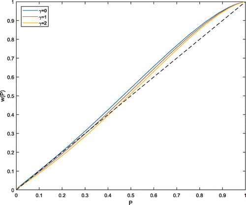
Using the estimated objective and risk-neutral densities, we can construct the probability weighting function for given utility function. We use the standard C.R.R.A. utility functions $u(R)=\frac{R^{1-\gamma }}{1-\gamma }$ for γ = 0 (linear utility), γ = 1 (logarithmic utility), and γ = 2 (power utility). We present estimates of the probability weighting function $w(P_{t,T})$ for one-month time horizon in Figure 5. It can be seen from the figure that the probability weighting function estimates have the S-shaped forms, implying that investors in the Hong Kong stock market underweight small probability events (tail events) and overweight large ones. The probability weighting functions obtained from Hong Kong index option market are different from those obtained from the U.S. index option market, which typically have the inverse-S shape (see Polkovnichenko & Zhao, 2013). The results call for further efforts to integrate the models that can account for S-shaped probability weighting in portfolio theory, asset pricing and risk management.

6. Conclusion

The study of the probability weighting function has been the focus of the financial economics literature. The probability weighting function has been extensively employed to model investor behaviour in financial markets. It is informative about the tail risk or crash risk of return dynamics and can provide explanation for tail risk premium. It can also be used to construct investor sentiment toward tail events and to construct probability weighting measures of tail events to capture investors’ decision weights toward tail events. In addition, the probability weighting function can be used to understand asset price dynamics and equity premium puzzle.

In this paper, we semi-parametrically estimate the pricing kernel from the Hong Kong index option market and obtain the empirical probability weighting functions based on the rank-dependent expected utility, using the non-affine G.A.R.C.H. diffusion model in a way that maintains the internal consistency of the objective and risk-neutral measures. Our results show that the empirical pricing kernel estimated from the Hong Kong index option market is non-monotonic, deviating from expected utility theory, and that the estimated probability weighting functions are S-shaped, which implies that investors underweight small probability events (tail events) and overweight large ones. The S-shaped probability weighting function with a utility function exhibiting C.R.R.A. based on the rand-dependent utility can explain the non-monotonicity of the pricing kernel. The results point to theoretical models with S-shaped probability weighting functions as a promising direction to understand asset price dynamics and further to explore implications for many economic issues, such as portfolio choices, asset pricing, and risk management.

Acknowledgements

We would like to thank the editor and two anonymous referees for their insightful and helpful comments and suggestions that greatly improved the paper.

Disclosure statement

No potential conflict of interest was reported by the author.

Additional information

Funding

This study was supported by the National Natural Science Foundation of China under Grant Nos. 71501001, 71401033 and 71431008; MOE (Ministry of Education in China) Project of Humanities and Social Sciences under Grant No. 14YJC790133; China Postdoctoral Science Foundation under Grant No. 2015M580416; Foreign Visiting Scholar Program for Excellent Youth Scholars in Universities under Grant No. gxfx2017031; Southern Jiangsu Capital Markets Research Center under Grant No. 2017ZSJD020.

Notes

1 Assuming that there are 250 trading days per year, then the time interval $\Delta t$ for one trading day is 1/250 year, and in this case the discretisation bias of Euler scheme is expected to be negligible.

Appendix A. Continuous stratified resampling

In the standard S.I.R. algorithm, the resampling is based on the discontinuous empirical distribution function $$\widehat{F}\left(h\right)=\sum _{i=1}^N{\pi }^{i}I(h-h^i)$$

where hⁱ, $i=1,\dots ,N,$ are sorted in ascending order, and ${\sum }_{i=1}^N{\pi }^i=1,$ I(z) is an indicator function, satisfying $$I\left(z\right)=\{\begin{array}{c}1,z>0\hfill \\ 0,z\le 0\hfill \end{array}$$

To produce samples of the state variables in a continuous way, Malik and Pitt (2011) approximate $\widehat{F}(h)$ by continuous empirical distribution function $\tilde{F}(h),$ which is given by $$\tilde{F}\left(h\right)={\omega }^{0}I(h^1<h)+{\omega }^{N}I(h^N<h)+\sum _{i=1}^{N-1}{\omega }^i{G}_i\left(\frac{h-h^i}{h^{i+1}-h^i}\right)$$

where ${\omega }^0={\pi }^1/2,{\omega }^N={\pi }^N/2,{\omega }^i=({\pi }^{i+1}+{\pi }^i)/2,i=1,2,\dots ,N-1,$ and $G_i(z)$ is a monotonically non-decreasing distribution function on $[0,1],$ such that $$G_i\left(z\right)=\{\begin{array}{c}0,z<0\hfill \\ z,0\le z\le 1\hfill \\ 1,z>1\hfill \end{array}$$

The above defined continuous distribution function $\tilde{F}(h)$ is easy to invert and thus sampling from it becomes very simple and quick. It can be shown that as $N\to \infty ,\tilde{F}(h)\to \widehat{F}(h)\to F(h),$ with F(h) being the true distribution function. In practice the difference between $\tilde{F}(h)$ and $\widehat{F}(h)$ becomes negligible for moderate N, typically we choose N = 500.

Continuous stratified resampling algorithm

First, we need to generate a single uniform $u\sim \mathit{UID}(0,1),$ and propagate sorted uniforms given by $$u_j=\frac{j-1}{N}+\frac{u}{N},j=1,2,\dots ,N$$

Then, we sample the index corresponding to the region which are sorted as $r^1,r^2,\dots r^N,$ and also produce a new set of uniforms, $u_1^{*},u_2^{*},\dots u_N^{*},$ according to the algorithm given below.

set $s=0,j=1;$

for $i=0:N$

$s=s+{\omega }^i;$

while ($u_j\le s j\le N$)

$r^j=i;$

$u_j^{*}=(u_j-(s-{\omega }^i))/{\omega }^i;$

$j=j+1;$

end

end

For the selected regions $r^1,r^2,\dots r^N,$ we set the new set of uniforms $u_1^{*},u_2^{*},\dots u_N^{*}$ as $$h^{j*}=\{\begin{array}{c}{h}^1,r^j=0\hfill \\ h^N,r^j=N\hfill \\ (h^{r^j+1}-h^{r^j})\times u_j^{*}+h^{r^j},\text{others}\hfill \end{array}$$

This produces as sample $h^{1*},h^{2*},\dots ,h^{N*}$ from continuous distribution function $\tilde{F}(h).$

Figure 1. Time-series and Q–Q plots of the H.S.I. returns. Source: Own calculation.

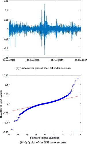
Figure 2. Filtered variances of the H.S.I. returns. Source: Own calculation.

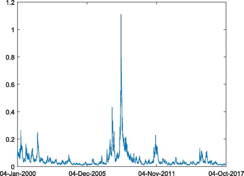
Figure 3. Estimates of objective and risk-neutral densities (O.D. and R.N.D.). Source: Own calculation.

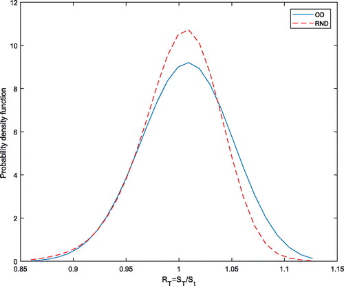
Figure 4. Empirical pricing kernel. Source: Own calculation.

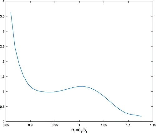
Figure 5. Estimates of probability weighting functions. Source: Own calculation.

References

- Aït-Sahalia, Y., & Lo, A. W. (2000). Nonparametric risk management and implied risk aversion. Journal of Econometrics, 94, 9–51.
- Audrino, F., & Meier, P. (2012). Empirical pricing kernel estimation using a functional gradient descent algorithm based on splines. Working Paper, University of St. Gallen.
- Bakshi, G., Madan, D., & Panayotov, G. (2010). Returns of claims on the upside and the viability of U-shaped pricing kernels. Journal of Financial Economics, 97(1), 130–154. doi: 10.1016/j.jfineco.2010.03.009
- Barberis, N., & Huang, M. (2008). Stocks as lotteries: The implications of probability weighting for security prices. American Economic Review, 98(5), 2066–2100. doi: 10.1257/aer.98.5.2066
- Barone-Adesi, G., Mancini, L., & Shefrin, H. (2017). Estimating sentiment, risk aversion, and time preference from behavioral pricing kernel theory. Working Paper, University of Lugano.
- Beare, B. K., & Schmidt, L. D. (2016). An empirical test of pricing kernel monotonicity. Journal of Applied Econometrics, 31(2), 338–356. doi: 10.1002/jae.2422
- Belomestny, D., Härdle, W. K., & Krymova, E. (2017). Sieve estimation of the minimal entropy martingale marginal density with application to pricing kernel estimation. International Journal of Theoretical and Applied Finance, 20(6), 1–21. doi: 10.1142/S0219024917500418
- Black, F. (1976). Studies of stock price volatility changes. In Proceedings of the 1976 meeting of business and economic statistics section. American Statistical Association, pp. 177–181.
- Bollerslev, T. (1986). Genearlized autoregressive conditional heteroskedasticity. Journal of Econometrics, 31(3), 307–327. doi: 10.1016/0304-4076(86)90063-1
- Bollerslev, T. (1987). A conditionally heteroskedastic time series model for speculative prices and rates of return. The Review of Economics and Statistics, 69(3), 542–547. doi: 10.2307/1925546
- Broadie, M., Chernov, M., & Johannes, M. (2007). Model specification and risk premia: Evidence from futures options. The Journal of Finance, 62(3), 1453–1490.
- Carr, P., & Madan, D. (1999). Option valuation using the fast Fourier transform. The Journal of Computational Finance, 2(4), 61–73. doi: 10.21314/JCF.1999.043
- Chabi-Yo, F. (2012). Pricing kernels with stochastic skewness and volatility risk. Management Science, 58(3), 624–640. doi: 10.1287/mnsc.1110.1424
- Chabi-Yo, F., Garcia, R., & Renault, E. (2008). State dependence can explain the risk aversion puzzle. Review of Financial Studies, 21(2), 973–1011. doi: 10.1093/rfs/hhm070
- Chabi-Yo, F., & Song, Z. G. (2013). Recovering the probability weights of tail events with volatility risk from option prices. Working Paper, Ohio State University.
- Chapman, D. (1997). Approximating the asset pricing kernel. Journal of Finance, 52(4), 1383–1410. doi: 10.1111/j.1540-6261.1997.tb01114.x
- Chernov, M. (2003). Empirical reverse engineering of the pricing kernel. Journal of Econometrics, 116(1-2), 329–364. doi: 10.1016/S0304-4076(03)00111-8
- Chernov, M., & Ghysels, E. (2000). A study towards a unified approach to the joint estimation of objective and risk neutral measures for the purpose of options valuation. Journal of Financial Economics, 56(3), 407–458. doi: 10.1016/S0304-405X(00)00046-5
- Christie, A. A. (1982). The stochastic behavior of common stock variances. Journal of Financial Economics, 10(4), 407–432. doi: 10.1016/0304-405X(82)90018-6
- Christoffersen, P., Heston, S., & Jacobs, K. (2013). Capturing option anomalies with a variance-dependent pricing kernel. Review of Financial Studies, 26(8), 1963–2006. doi: 10.1093/rfs/hht033
- Christoffersen, P., Jacobs, K., & Mimouni, K. (2010). Volatility dynamics for the S&P 500: Evidence from realized volatility, daily returns, and option prices. The Review of Financial Studies, 23(8), 3141–3189.
- Cochrane, J. H. (2001). Asset pricing. New Jersey: Princeton University Press.
- Cuesdeanu, H., & Jackwerth, J. C. (2016). The pricing kernel puzzle in forward looking data. Working Paper, University of Konstanz.
- Detlefsen, K., Härdle, W., & Moro, R. (2007). Empirical pricing kernels and investor preferences. Working Paper, Universite de Provence.
- Dierkes, M. (2009). Option-implied risk attitude under rank-dependent utility. Working Paper, University of Münster.
- Dierkes, M. (2013). Probability weighting and asset prices. Working Paper, University of Münster.
- Duan, J. C., & Fulop, A. (2009). Estimating the structural credit risk model when equity prices are contaminated by trading noises. Journal of Econometrics, 150(2), 288–296. doi: 10.1016/j.jeconom.2008.12.003
- Figlewski, S., & Malik, M. F. (2014). Options on leveraged ETFs: A window on investor heterogeneity. Working Paper, New York University.
- Gollier, C. (2011). Portfolio choices and asset prices: The comparative statics of ambiguity aversion. The Review of Economic Studies, 78(4), 1329–1344. doi: 10.1093/restud/rdr013
- Golubev, Y., Härdle, W., & Timofeev, R. (2014). Testing monotonicity of pricing kernels. AStA Advances in Statistical Analysis, 98(4), 305–326. doi: 10.1007/s10182-014-0225-5
- Gordon, N. J., Salmond, D. J., & Smith, A. F. (1993). Novel approach to nonlinear/non-Gaussian Bayesian state estimation. IEE Proceedings F Radar and Signal Processing, 140(2), 107–113. doi: 10.1049/ip-f-2.1993.0015
- Hansen, L. P., & Jagannathan, R. (1991). Implications of security market data for models of dynamic economies. Journal of Political Economy, 99, (2), 225–262. doi: 10.1086/261749
- Härdle, W. K., Okhrin, Y., & Wang, W. (2015). Uniform confidence bands for pricing kernels. Journal of Financial Econometrics, 13(2), 376–413. doi: 10.1093/jjfinec/nbu002
- Heston, S. L. (1993). A closed-form solution for options with stochastic volatility with applications to bond and currency options. Review of Financial Studies, 6(2), 327–343. doi: 10.1093/rfs/6.2.327
- Jackwerth, J. (2000). Recovering risk aversion from option prices and realized returns. Review of Financial Studies, 13(2), 433–451. doi: 10.1093/rfs/13.2.433
- Kaeck, A., & Alexander, C. (2013). Stochastic volatility jump-diffusions for European equity index dynamics. European Financial Management, 19(3), 470–496.
- Kliger, D., & Levy, O. (2009). Theories of choice under risk: Insights from financial markets. Journal of Economic Behavior and Organization, 71(2), 330–346. doi: 10.1016/j.jebo.2009.01.012
- Malik, S., & Pitt, M. K. (2011). Particle filters for continuous likelihood evaluation and maximization. Journal of Econometrics, 165(2), 190–209. doi: 10.1016/j.jeconom.2011.07.006
- Pitt, M. K., Malik, S., & Doucet, A. (2014). Simulated likelihood inference for stochastic volatility models using continuous particle filtering. Annals of the Institute of Statistical Mathematics, 66(3), 527–552. doi: 10.1007/s10463-014-0456-y
- Polkovnichenko, V. (2005). Household portfolio diversification: A case for rank-dependent preferences. Review of Financial Studies, 18(4), 1467–1502. doi: 10.1093/rfs/hhi033
- Polkovnichenko, V., & Zhao, F. (2013). Probability weighting functions implied in options prices. Journal of Financial Economics, 107(3), 580–609. doi: 10.1016/j.jfineco.2012.09.008
- Prelec, D. (1998). The probability weighting function. Econometrica, 66(3), 497–527. doi: 10.2307/2998573
- Quiggin, J. (1993). Generalized expected utility theory: The rank-dependent model. Norwell, MA, Dordrecht, the Netherlands: Kluwer Academic Publishers.
- Rosenberg, J., & Engle, R. F. (2002). Empirical pricing kernels. Journal of Financial Economics, 64(3), 341–372. doi: 10.1016/S0304-405X(02)00128-9
- Shefrin, H., & Statman, M. (2000). Behavioral portfolio theory. Journal of Financial and Quantitative Analysis, 35(2), 127–151. doi: 10.2307/2676187
- Song, Z. G., & Xiu, D. C. (2016). A tale of two option markets: Pricing kernels and volatility risk. Journal of Econometrics, 190(1), 176–196.
- Tversky, A., & Kahneman, D. (1992). Advances in prospect theory: Cumulative representation of uncertainty. Journal of Risk and Uncertainty, 5(4), 297–323. doi: 10.1007/BF00122574
- Wang, B. (2017). Probability weighting and asset prices: Evidence from mergers and acquisitions. Working Paper, Fordham University.
- Wu, X. Y., Ma, C. Q., & Wang, S. Y. (2012). Warrant pricing under GARCH diffusion model. Economic Modelling, 29(6), 2237–2244. doi: 10.1016/j.econmod.2012.06.020
- Wu, X. Y., Zhou, H. L., & Wang, S. Y. (Forthcoming). Estimation of market prices of risks in G.A.R.C.H. diffusion model. Economic Research-Ekonomska Istraživanja, doi: 10.1080/1331677X.2017.1421989
- Yang, H., & Kanniainen, J. (2017). Jump and volatility dynamics for the S&P 500: Evidence for infinite-activity jumps with non-affine volatility dynamics from stock and option markets. Review of Finance, 21(2), 811–844. doi: 10.1093/rof/rfw001
- Ziegler, A. (2007). Why does implied risk aversion smile? Review of Financial Studies, 20(3), 859–904. doi: 10.1093/rfs/hhl023