Does the inflow of remittances cause environmental degradation? Empirical evidence from China

Abstract

Remittances inflow plays a significant role in promoting the economic welfare of a country; it has a multidimensional effect on the economy and links with the carbon emissions. This study examines the possible asymmetric transmissions from remittances to carbon dioxide emissions (CO2) in China using time series data from 1980 to 2014. The Non-linear NARDL method is employed to check the longrun asymmetric relationship between remittances inflow and carbon emissions. The findings show that a positive shock in remittances causes an increase in CO2 emissions, while a negative shock in remittances causes a decrease in CO2 emissions. The results support the existence of an asymmetric cointegrating relationship between remittances and CO2 emissions in both short run and the long run. The NARDL dynamic multiplier graph assumes that positive remittances shocks are highe compared to the negative remittances shocks. It suggests that policymakers in China should consider remittances as a policy instrument especially designing strategies and policies related to sustainable environmental quality in the long run.

Keywords:

• CO2 emissions
• remittances
• NARDL modeling dynamic multiplier
• positive shocks
• negative shocks

JEL Codes:

• Q50
• C32
• F24

1. Introduction

Remittances are the primary source of international financial resources in the world, which sometimes are responsible for an increase in foreign direct investment. Remittances inflow is not only a new financial phenomenon, but it is considered as a significant source of income due to its economic influence worldwide (Meyer & Shera 2017). The size of remittances inflow is three times larger than the value of official development assistance and has a positive impact on human welfare and development. Remittances inflow is the primary source of alleviating poverty and providing financial capital to impecunious families for initiating a small business (Second International Handbook on Globalisation, Education and Policy Research, 2015). Beside microeconomic variables it also affects the macroeconomic variables and has a positive effect on bridging the deficit in the balance of payments (BOP). This influence of remittances inflow is relatively high and more critical in low-income economies where it leads an increase in credit ratings (Hijazi, 2016).

Remittances also play a significant role in promoting financial development. The rise in remittances inflow leads to an increase in demand for financial services either during savings of money or transfer of money. In addition to this, it is a source of providing capital to the business community which is unable to finance from commercial banks at a low rate (Motelle, 2011). Remittances support small firms by providing capital and also promote domestic investment which further promotes the financial development of a country. Similarly, expansions in businesses through remittances does have a role in causing damage to the environment. During the last few years, many researchers have conducted surveys on the issue of “Impact of Financial Development on Carbon Emission.” For instance, (Ayeche, Barhoumi, & Amin, 2016; Başarir & Çakir, 2015; Farhani & Ozturk, 2015; Li, Zhang, & Ma, 2015; Mugableh, 2015) concluded that financial development increases the level of carbon emissions. Two main factors can elaborate on the impact of financial development on environmental degradation. First, improvement of stock market listed companies to cut back on their financial expenses, increase credit channels and extend operational risk, which sequentially makes firms capable of enhanced finance, set up the latest resources and escalate their production volume, thus increasing the level of CO2 emissions.

China is the second largest remittances receiver country placed equal second with India. In 2016, China received 16.1 billion dollars in remittances from other parts of the world (World Bank Group, 2017). Similar to other countries, China remittances inflow is utilised for different purposes including consumption, investment, and savings. Investment is a source of financial development in the case of China, but which might have an adverse effect on the environment. Expansion of financial development in China is linked to increasing carbon emissions. The current study investigates the possible relationship between remittances and CO2 emissions. Thus, this paper attempts to fill the gap in the existing literature by taking remittances as a powerful tool of financial development and economic growth and tries to examine its indirect role in CO2 emissions. The rest of the paper divided into a conceptual framework, data source, methodology, results, discussions, and conclusions.

2. Conceptual framework

a. Pollution and CO2 problem

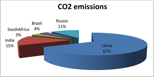
It is not surprising that the per capita CO2 emissions of China are more than 87% of the global average and 33% ahead of the level of the OECD economies. The main problem is the increasing growth rate of China’s per capita CO2 emissions. There is consent in the scientific community that the level of aggregate CO2 in the atmosphere should not go beyond a level equal to two times the level prevailing before the industrial revolution (Pacala & Socolow, 2004). In 2010, China has turned out to be the largest carbon discharger, surpassing the U.S.A. and the largest end user of fossil fuels in 2011. CO2 emissions in China have reached around nine billion tonnes by 2011, 23% of the total emissions in the world. While CO2 emissions from the use of fossil fuel burning and production of cement reached 8.50 Gt CO2 in 2012, it is worth mentioning that China’s CO2 emanations were only 5.46 Mt CO2 in 1950; hence the total discharges escalated more than 100-fold over 60 years. For example, the growth rate was the topmost among the globally significant countries (Liu, 2016). On the other hand, exceeding that level could bring about fiercely changeable weather, protracted droughts, and melting glaciers. If the rate of increase in future emissions is as prolonged as it was in the last 30 years, this perilous level could be reached in 50 years’ time. Consequently, CO2 emissions are a severe and burning issue (Chow, 2014). Figure 1 depicts that China is the most CO2 emitter among emerging economies (BRICS).

Figure 1. CO2 in the emerging economies.

Air pollution and energy use have been synonymous in China for many years, particularly in urban areas. In many big cities, air pollution is also common because a major amount of industry relies on coal is situated in the rural areas. Twenty years ago in China’s northern cities, such as Shenyang, air pollution was depicted by declined visibility caused by the high levels of particulates and other contaminated gases. Even though conditions have improved in advanced and modern cities like Shanghai and Beijing, still China has three of the ten most polluted cities in the world, and more than a hundred cities do not meet the World Health Organization (WHO) air quality parameters (Chinese Academy of Sciences, 2005). On the other hand, with the rise in pollution treatment, some conventional pollutants are controlled to some extent. However, new pollution problems keep evolving. For instance, with the rising awareness of the global environment and the unceasing emergence of climate change effects, the discharge of greenhouse gases has been steadily integrated into the country’s environmental agenda (Chang, 2011)

b. The relationship between remittances and CO2 emissions

As the literature on the relationship between remittances and CO2 are not available, we will explain this relationship with the help of a five-stage-interaction-mechanism. In the first stage, remittances increase household per capita income, which further increases the consumption and savings levels of households. A study was conducted by Prabal and Dilip (2012) on the relationship between remittances and household income. Their findings reveal that on average the remittances increase income level and consumption level of the household. Another study was carried out by Iheke (2012) on the impact of remittances on per capita income from the perspective of the Nigerian economy. The results depicted that remittances improve per capita income and hence households could consume even more., while Balde (2011) infers that remittances not only swell the level of savings but also increase the level of investment. In the second stage, increase in consumption and savings leads to an increase in aggregate demand and bank deposits (Arnold, 2008; Bhole, 2009; Graziani, 2003; Herendeen, 2007; Sawyer & Sprinkle, 2015; Sexton, 2015; Tregarthen & Rittenberg, 1999). In the third stage, increases in aggregate demand and bank deposits increases industrial production and also improves the financial sector (Corsepius, 1989; Hahnel, 1999; Herr & Kazandziska, 2011; Tregarthen & Rittenberg, 1999; Tucker, 2008). It is noteworthy to mention that this stage is also responsible for the increase in CO2 emissions, because the increase in industrial production leads to an increase in the use of energy, which is one of the prime causes of greenhouse gases. On the other hand, financial developments are also responsible for the increase in CO2 emissions. Many scholars and academics have probed the connection between financial development and CO2 emissions for different economies. The findings showed that financial development increases the emissions of CO2. These studies include (Boutabba, 2014; Jamel & Maktouf, 2017; Li, Zhang, & Ma, 2015; Ozturk & Acaravci, 2013; Saboori, Sulaiman, & Mohd, 2012; Zhang, 2011), while some studies found a negative relationship between financial development and CO2 emissions. These studies include (Mulali, Tang, & Oztur, 2015; Saidi & Mbarek, 2017; Xing, Jiang, & Ma, 2017). In the fourth stage, financial development and industrial production positively contribute to economic growth (Ang, 2008; Kedourie, 2013; Lakhera, 2016; Malinvaud, 1979; Sentā, 1966; Shucheng, 2017; Swanson & Lin, 2009) . In the fifth stage, economic growth leads to an increase in CO2 emissions. Many researchers have carried out studies on the relationships between economic growth and CO2 emissions. Their results also concluded both the positive and negative impact of economic development and CO2 emissions. These studies comprise (De Bruyn, van den Bergh, & Opschoor, 1998; Dinda, 2004; Friedl & Getzner, 2003; Grossman & Krueger, 1995; Heil & Selden, 2001; Holtz-Eakin & Selden, 1995; Managi & Jena, 2008; Moomaw & Unruh, 1997; Obradovic & Lojanica, 2017; Ozturk & Uddin, 2012; Selden & Song, 1994; Stern, 2004).

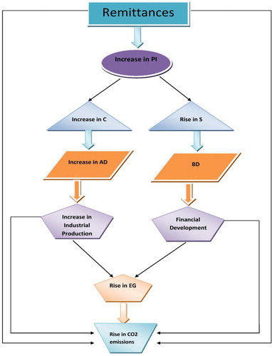
Thus, remittances as main determinants of financial development and economic growth contribute in emissions of CO2 through a five-stage-interaction-mechanism. It means remittances do not directly affect CO2 emissions, rather through different stages. The five-stages-remittances-CO2-interaction-mechanism is also represented in Figure 2.

Figure 2. The Indirect connection between Remittances and CO2 emissions. Notes: PI = Personel Income; C = Consumption; S = Savings; AD = Aggregate Demand; BD = Bank Deposits; EG = Economic Growth.

c. Five-stages-interaction-mechanism (FSIM): how remittances causes environmental degradation?

In the above section, we introduced the concept of FSIM. In this part, we discuss this concept in more detail. FSIM elaborates that inflow of remittances is an essential factor that determines CO2 emissions. Furthermore, FSIM is based on the following five stages that explain the interaction mechanism between the inflow of remittances and CO2 emissions.

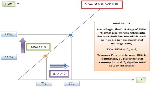
Stage 1: Inflow of remittances leads an increase in household income

Developing economies are characterised by lack of basic infrastructure, lack of technology and capital, underutilised natural resources, the vicious circle of poverty, high population growth rate, high unemployment rate, low literacy rate, etc. Moreover, due to the low per capita income and fewer job opportunities in developing economies, people move to other countries to earn a higher income. Thus, residents of developing countries work and earn money. To support their family, they send money to their home country. This money in the form of remittances (REM) boosts their families’ total income.

The nexus between the inflow of remittances and household income is depicted in Figure 3. At the initial position, remittances and household income are ${\mathit{REM}}_0$ and${\mathit{TY}}_0$, respectively, while inflow of remittances brings a change in household income from$\mathrm{ }{\mathit{TY}}_0$ and ${\mathit{TY}}_1$. This response is called first stage of FSTM.

Figure 3. First stage of FSIM.

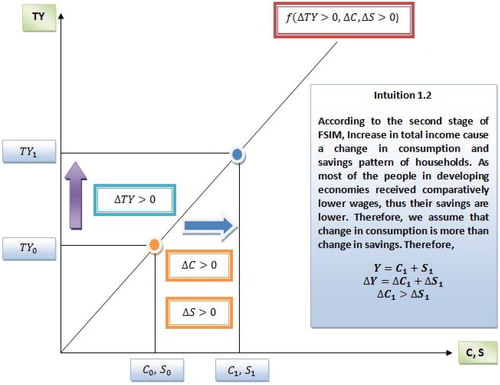
Stage 2: Increase in household total income leads an increase in consumption and savings

The household divides its income into two parts. The first part consists of consumption. Every individual works to earn money to consume goods and services. An ordinary consumer spends money on both durable and non-durable goods. These goods include daily use items which are necessary not for survival but to also make their lives more comfortable. The second part of income is savings. In developing economies, the economic condition is uncertain. People feel fear that they will lose their jobs. Meanwhile, the average price level is also changeable. This situation makes people save money to meet future demands.

The relationship between total income which is increased due to the inflow of remittances and consumption-savings is presented in Figure 4. As the level of income increases from ${\mathit{TY}}_0$ to ${\mathit{TY}}_1$ this leads an increase in the level of household consumption from $C_0$ to $C_1$ and level of savings from $S_0$ to $S_1$. This nexus between household income (TY + REM) and consumption-saving is called the second stage of FSIM.

Figure 4. Second stage of FSIM.

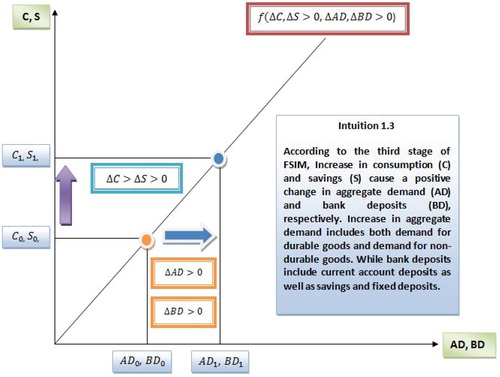
Stage 3: Increase in consumption and savings leads an increase in aggregate demand and bank savings, respectively

Consumption and savings are essential factors that determine economic growth in both the short run and long run. The demand for goods comes from the household. Any changes in the pattern of aggregate consumption have a profound influence on aggregate demand. Moreover, household utilises the more significant portion of remittances on consuming goods, which further increases aggregate demand. Also, rational families deposit their surplus money in banks to meet their future economic desires. Thus, any variation in savings causes drastic changes in bank deposits.

The possible connection between consumption-savings and aggregate demand-bank deposits is depicted in Figure 5. Increase in C-S from $C_{0,\mathrm{ }}{S}_{0,\mathrm{ }}$ to $C_{1,\mathrm{ }}{S}_{1,\mathrm{ }}$ leads to an upsurge in level of the AD-BD from ${\mathit{AD}}_{0,\mathrm{ }}{\mathit{BD}}_{0,\mathrm{ }}$ to ${\mathit{AD}}_{1,\mathrm{ }}{\mathit{BD}}_{1,\mathrm{ }}$. This nexus between C-S (C = f (TY, REM), S = f(TY, REM)) and AD-BD is called the third stage of FSIM.

Figure 5. Third stage of FSIM.

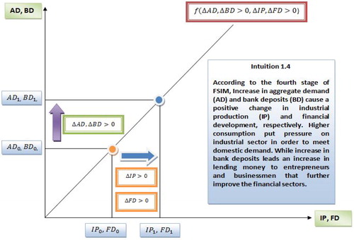
Stage 4: Increase in aggregate demand and bank savings leads an increase in industrial production and improve financial sector

Financial sectors and industrialisation are interconnected, because financial institutions provide short-term as well as long-term loans to entrepreneurs to open a factory or construct a new plant. Remittances are considered one of the vital factors of financial development. A persistent increase in remittance leads an increase in aggregate demand and bank savings. Moreover, to meet the domestic demand, the industrial sector also increases the level of production, while banking sectors increase their lending to the business community, which further improves the financial sectors.

Figure 6 depicts the linkage between AD-BD and IP-FD. A rise in AD-BD from ${\mathit{AD}}_{0,\mathrm{ }}{\mathit{BD}}_{0,\mathrm{ }}$ to ${\mathit{AD}}_{1,\mathrm{ }}{\mathit{BD}}_{1,\mathrm{ }}$ brings a change in the level of IP-FD from ${\mathit{IP}}_{0,\mathrm{ }}{\mathit{FD}}_{0,\mathrm{ }}$ to ${\mathit{IP}}_{1,\mathrm{ }}{\mathit{FD}}_{1,}$. This nexus between AD-BD and AD-BD is called the fourth stage of FSIM.

Figure 6. The Fourth stage of FSIM.

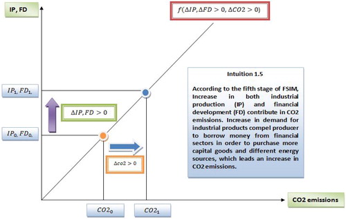
Stage 5: Increase in both industrial production and financial development contribute to CO2 emissions

Industrial production and financial development are two important sources of carbon dioxide emissions. Different sources of energy are used to produce goods. These sources include oil, natural gas, coal, etc. All these sources contribute to emissions of CO2. Thus, a rise in industrial production leads to an increase in utilisation of fossils fuel which ultimately result in a high amount of emissions. On the other hand, financial development is also responsible for contaminating the environment by providing an opportunity for heavy industries which use inefficient production technology.

Figure 7 signifies the nexus between IP-FD and CO2 emissions. A rise in IP-FD from ${\mathit{IP}}_{0,\mathrm{ }}{\mathit{FD}}_{0,\mathrm{ }}$ to ${\mathit{IP}}_{1,\mathrm{ }}{\mathit{FD}}_{1,\mathrm{ }}$ brings a change in the level of CO2 from ${\mathit{CO}2}_{0,\mathrm{ }}$ to${\mathit{CO}2}_{1,\mathrm{ }}$. This nexus between IP-FD and Co2 is called the fifth stage of FSIM. The fifth stage is the result of the last four stages where remittances are the main elements which bring a variation in carbon dioxide emissions.

Figure 7. The Fifth stage of FSIM.

Figure 6 shows the derivation of the FSIM curve. It is clear from the figure that the increase in remittances from ${\mathit{REM}}_0$ to ${\mathit{REM}}_1$ brings an upsurge in CO2 emissions from ${\mathit{CO}2}_0$ to ${\mathit{CO}2}_1$ through different stages. By joining points K and L in the last panel of Figure 8, we get the FSIM curve. It is noted that the FSIM curve signifies an indirect positive relationship between inflow of remittances and CO2 emissions. In short, the FSIM curve elaborates how the inflow of remittances affects the environment through five different stages.

Figure 8. Derivation of FSIM curve.

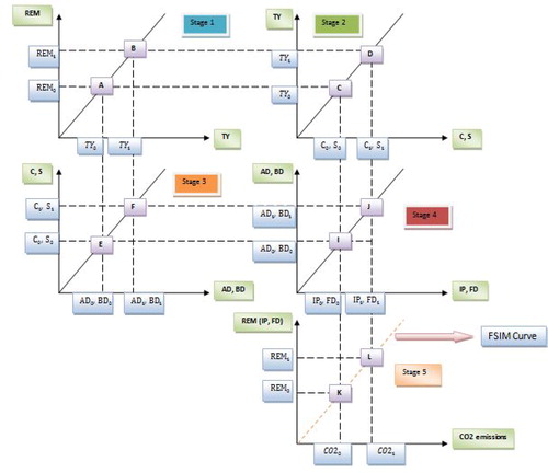
Figure 9. Relationships between negative shocks in inflow of remittances and CO2 emissions.

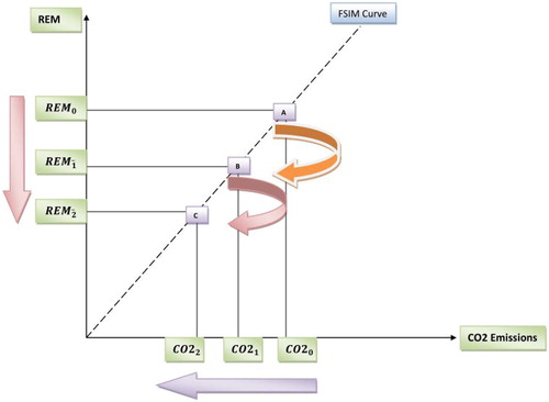
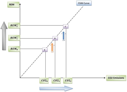
d. Positive and negative shocks in remittances and CO2 emissions

Labour migration is an important factor that determines inflow of remittances. While labour migration from one country to another country relies on economic activities, any changes in economic activities may bring a drastic change in the labour market which has further effect on inflow of remittances. Let us suppose there is a decrease in an economic activities which further trim down the inflow of remittances from ${\mathit{REM}}_0$ to ${\mathit{REM}}_1^{+}$ which leads to a decrease in carbon emissions from ${\mathit{CO}2}_0$ to ${\mathit{CO}2}_1$ (see Figure 9).

Due to contractions in economic activities, many workers become unemployed and are unable to send remittances to their home country. Thus, decrease in inflow of remittances leads a decrease in household income, savings, aggregate demand, bank deposits, lending money, and industrial production. Further, decline in industrial production will decrease CO2 emissions. Therefore, negative shocks in inflow of remittances leads to a reduction in carbon emissions. On the other hand, positive shocks lead an increase in carbon emissions.

The relationships between positive shocks in remittances and carbon emissions are presented in Figure 10. A rise in remittances from ${\mathit{REM}}_0$ to ${\mathit{REM}}_2^{+}$ leads an increase in carbon emissions from ${\mathit{CO}2}_0$ to ${\mathit{CO}2}_2$.

Figure 10. Relationships between positive shocks in inflow of remittances and CO2 emissions.

3. Data source and methodology

This study inspects the association between remittances and CO2 emissions by taking time series data from 1980 to 2014. All the data on variables have been collected from the World Bank database. The annual remittances are given in current U.S. dollars, and CO2 emissions are denoted in Kiloton. Eviews 10 is used for data analysis.

The originality of this study is based on two considerations. First we have studied remittances as a determinant of CO2 emissions for the first time. Secondly, we have employed the NARDL model, which is recently introduced by (Shin, Yu, & Greenwoo, 2013). This method allows us to scrutinise the short-run and long-run asymmetrical effects of positive and negative components of remittances on the CO2 emissions in the context of China. The non-linear ARDL model is an expanded version of the linear ARDL (Pesaran, Shin, & Smith, 2001). This model helps to capture the asymmetries emerging due to change in economic policy or business cycle. One of the most important advantages of this model is that it can be applied at any case of order of integration except I(2) (Pesaran, Shin, & Smith, 2001). Hence, the ARDL model can be applied in order to test the possible existence of long run and short run associations among variables included in the model without any earlier information about the order of integration of the single variables included in the model, which do not cause problems associated with the pre-time series stationary process (Nusair, 2016). The other advantages of the ARDL technique is that it can be applied on small sample size and both dependent and independent variables can be employed in the model with lags (Caporale & Pittis 1999; Pesaran & Shin 1999). Due to its multiple advantages, the NARDL technique has been used by many researchers in order to identify asymmetries arising due to economic shock. These studies include (Alsamara et al., 2017; Bagnai & Ospina 2016; Elafif et al., 2017; Mamun et al., 2016; Pal & Mitra 2015, 2016; Salisu & Isah 2017; Shin et al., 2018). The relationship between inflow of remittances and CO2 emissions is expressed in the following functional form: (1) $$\mathit{CO}{2}_t=f\left(\mathit{RE}{M}_t\right)\mathrm{ }$$(1)

For modelling purpose, we express equation (1)(1) $$\mathit{CO}{2}_t=f\left(\mathit{RE}{M}_t\right)\mathrm{ }$$(1) into Cobb-Douglas format:

(2) $$\mathit{CO}{2}_t={\vartheta }_0{\mathit{REM}}_t^{\vartheta }{e}^{u_t}\mathrm{ }$$(2)

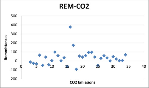
In our model, we are presuming a linear association between inflow of remittances and CO2 emissions. But the actual situation is different. Figure 11 signifies that the linkage between inflow of remittances and CO2 emissions is slightly non-linear for China. Thus it may be expected that the positive and negative shocks in remittances have deep impact on CO2 emissions. Therefore, we modify equation (2)(2) $$\mathit{CO}{2}_t={\vartheta }_0{\mathit{REM}}_t^{\vartheta }{e}^{u_t}\mathrm{ }$$(2) as follows: (3) $$\mathit{CO}{2}_t={\vartheta }_0{\mathit{REM}}_t^{+{\vartheta }_1}{\mathit{REM}}_t^{-{\vartheta }_1}{e}^{{\mathrm{\epsilon }}_{\mathrm{t}}}\mathrm{ }$$(3)

Figure 11. Relationship between Remittances and CO2 emissions for China.

This can be expressed in log form: (4) $${\mathrm{GCO}2}_{\mathrm{t}}={\mathrm{\vartheta }}_0+{\mathrm{\vartheta }}_1^{+}\mathrm{G}{\mathrm{REM}}_{\mathrm{t}}^{+}+{\mathrm{\vartheta }}_2^{-}{\mathrm{GREM}}_{\mathrm{t}}^{-}+{\mathrm{\epsilon }}_{\mathrm{t}}\mathrm{ }$$(4)

where G represents growth rate between previous and current year, $\mathrm{CO}2$ is carbon emissions integrating of order one, $\mathrm{REM}$ represents remittances integrating of order one, $\mathrm{\vartheta }={\mathrm{\vartheta }}_0,\mathrm{ }{\mathrm{\vartheta }}_1^{+},\mathrm{ }{\mathrm{\vartheta }}_2^{-})$ is a vector of long-run unknown parameters. It is noted that ${\mathrm{\vartheta }}_1^{+}$ represents coefficients of positive component of remittances and ${\mathrm{\vartheta }}_2^{-}$ indicates the negative component of remittances. While${\mathrm{REM}}_{\mathrm{t}}={\mathrm{REM}}_0+{\mathrm{REM}}_{\mathrm{t}}^{+}+{\mathrm{REM}}_{\mathrm{t}}^{-}$. Where ${\mathrm{REM}}_{\mathrm{t}}^{+}$ and ${\mathrm{REM}}_{\mathrm{t}}^{-}$ are partial sum process of positive and negative variation in ${\mathrm{REM}}_{\mathrm{t}}$ follow as; (5) $${\mathrm{REM}}_{\mathrm{t}}^{+}=\sum _{\mathrm{j}=1}^{\mathrm{t}}\Delta {\mathrm{REM}}_{\mathrm{j}}^{+}=\sum _{\mathrm{j}=1}^{\mathrm{t}}\mathrm{max }\left(\Delta {\mathrm{REM}}_{\mathrm{j}},\mathrm{ }0\right),\mathrm{ }{\mathrm{REM}}_{\mathrm{t}}^{-}=\sum _{\mathrm{j}=1}^{\mathrm{t}}\Delta {\mathrm{REM}}_{\mathrm{j}}^{-}=\sum _{\mathrm{j}=1}^{\mathrm{t}}\mathrm{min }\left(\Delta {\mathrm{REM}}_{\mathrm{j}},\mathrm{ }0\right)\mathrm{ }$$(5)

The equation (5)(5) $${\mathrm{REM}}_{\mathrm{t}}^{+}=\sum _{\mathrm{j}=1}^{\mathrm{t}}\Delta {\mathrm{REM}}_{\mathrm{j}}^{+}=\sum _{\mathrm{j}=1}^{\mathrm{t}}\mathrm{max }\left(\Delta {\mathrm{REM}}_{\mathrm{j}},\mathrm{ }0\right),\mathrm{ }{\mathrm{REM}}_{\mathrm{t}}^{-}=\sum _{\mathrm{j}=1}^{\mathrm{t}}\Delta {\mathrm{REM}}_{\mathrm{j}}^{-}=\sum _{\mathrm{j}=1}^{\mathrm{t}}\mathrm{min }\left(\Delta {\mathrm{REM}}_{\mathrm{j}},\mathrm{ }0\right)\mathrm{ }$$(5) is a simple modelling in order to study asymmetrical behaviour among variables. This modelling was first employed by (Schorderet, 2001) from the perspective of non-linear nexus between unemployment and output.

The concept of hidden co-integration was developed by (Granger & Yoon, 2002). They defined cointegration as both positive and negative components of the main variables in the context of the connection between United States of America short and long term rates of interest and output-employment nexus. Later, Schorderet, 2003) simplifies this idea and elaborates the following linear combination of partial sum components having the property of stationarity; (6) $${\zeta }_t={\mathrm{\Psi }}_0^{+}{\mathit{CO}2}_t^{+}+{\mathrm{\Psi }}_0^{-}{\mathit{CO}2}_t^{-}+{\mathrm{\Psi }}_1^{+}{\mathit{REM}}_t^{+}+{\mathrm{\Psi }}_1^{-}{\mathit{REM}}_t^{-}\mathrm{ }$$(6)

where ${\mathit{CO}2}_t$ and ${\mathit{REM}}_t$ are considered to be “Asymmetrical Cointegration” if ${\zeta }_t$ is stationary. It infers that symmetric cointegration is a unique case of equation (6)(6) $${\zeta }_t={\mathrm{\Psi }}_0^{+}{\mathit{CO}2}_t^{+}+{\mathrm{\Psi }}_0^{-}{\mathit{CO}2}_t^{-}+{\mathrm{\Psi }}_1^{+}{\mathit{REM}}_t^{+}+{\mathrm{\Psi }}_1^{-}{\mathit{REM}}_t^{-}\mathrm{ }$$(6) , taken only if ${\mathrm{\Psi }}_0^{+}={\mathrm{\Psi }}_0^{-}$ and ${\mathrm{\Psi }}_1^{+}={\mathrm{\Psi }}_1^{-}$. Following (Shin, Yu, & Greenwoo, 2013), to avoid our model from the problem of hidden cointegration we impose the following restrictions on equation (6)(6) $${\zeta }_t={\mathrm{\Psi }}_0^{+}{\mathit{CO}2}_t^{+}+{\mathrm{\Psi }}_0^{-}{\mathit{CO}2}_t^{-}+{\mathrm{\Psi }}_1^{+}{\mathit{REM}}_t^{+}+{\mathrm{\Psi }}_1^{-}{\mathit{REM}}_t^{-}\mathrm{ }$$(6) such as ${\mathrm{\Psi }}_0^{+}={\mathrm{\Psi }}_0^{-}={\mathrm{\Psi }}_0$, ${\psi }^{+}=\frac{{-\psi }_1^{+}}{{\mathrm{\Psi }}_0^{+}}$ and ${\psi }^{-}=\frac{{-\psi }_1^{-}}{{\mathrm{\Psi }}_0^{+}}$.

Following (Shin, Yu, & Greenwoo, 2013), Equation (3)(3) $$\mathit{CO}{2}_t={\vartheta }_0{\mathit{REM}}_t^{+{\vartheta }_1}{\mathit{REM}}_t^{-{\vartheta }_1}{e}^{{\mathrm{\epsilon }}_{\mathrm{t}}}\mathrm{ }$$(3) can be fitted in an ARDL setting under the context of (Pesaran et al., 1998, 2001) as: (7) $${\Delta \mathrm{CO}2}_{\mathrm{t}}={\mathrm{\varsigma }}_0+{\mathrm{\varsigma }}_1{\mathrm{CO}2}_{\mathrm{t}-\mathrm{i}}+{\mathrm{\varsigma }}_2^{+}{\mathrm{REM}}_{\mathrm{t}-\mathrm{i}}^{+}+{\mathrm{\varsigma }}_3^{-}{\mathrm{REM}}_{\mathrm{t}-\mathrm{i}}^{-}+\sum _{\mathrm{i}=1}^{\mathrm{p}}{\mathrm{\Theta }}_{\mathrm{i}}{\Delta \mathrm{CO}2}_{\mathrm{t}-\mathrm{i}}+\mathrm{ }\sum _{\mathrm{i}=0}^{\mathrm{m}}({\mathrm{\varpi }}_{\mathrm{i}}^{+}\Delta {\mathrm{REM}}_{\mathrm{t}-\mathrm{i}}^{+}+\mathrm{ }{\mathrm{\varpi }}_{\mathrm{i}}^{-}\Delta {\mathrm{REM}}_{\mathrm{t}-\mathrm{i}}^{-})+{\mathrm{ϵ}}_{\mathrm{t}}\mathrm{ }$$(7)

where $p$ and $\mathrm{m}$ are lag orders.$\mathrm{ }{\sum }_{\mathrm{i}=0}^{\mathrm{m}}{\mathrm{\varpi }}_{\mathrm{i}}^{+}$ estimates the short-run possible response of remittances increases in the CO2 emissions while ${\sum }_{\mathrm{i}=0}^{\mathrm{m}}{\mathrm{\varpi }}_{\mathrm{i}}^{-}$ measures the short run impact of remittances reduction on CO2 emissions. Hence, in this setup, along with asymmetric long-term association, the asymmetric short-run impact of variations in remittances on CO2 emissions is also captured.

The error correction model (ECM) of the previous equation is depicted as: (8) $${\Delta \mathrm{CO}2}_{\mathrm{t}}=\sum _{\mathrm{i}=1}^{\mathrm{p}}{\mathrm{{\rm A}}}_{\mathrm{i}}{\Delta \mathrm{CO}2}_{\mathrm{t}-\mathrm{i}}+\sum _{\mathrm{i}=1}^{\mathrm{m}}{(\mathrm{\eta }}_{\mathrm{i}}^{+}\Delta {\mathrm{REM}}_{\mathrm{t}-\mathrm{i}}^{+}+{\mathrm{\eta }}_{\mathrm{i}}^{-}\Delta {\mathrm{REM}}_{\mathrm{t}-\mathrm{i}}^{-})+{\mathrm{{\rm Y}}}_{\mathrm{i}}{\mathrm{ECT}}_{\mathrm{t}-\mathrm{i}}+{\mathrm{\rho }}_{\mathrm{t}}\mathrm{ }$$(8)

where ${\mathrm{{\rm A}}}_{\mathrm{i}}$, depicts short-run coefficient and ${\mathrm{\eta }}_{\mathrm{i}}^{+}$, ${\mathrm{\eta }}_{\mathrm{i}}^{-}$ indicate short-run adjustment symmetry, while ${\mathrm{{\rm Y}}}_{\mathrm{i}}$ indicates the coefficient of error correction term.

We follow the following steps and procedures in order to estimate the NARDL model. In step 1, we identify the order of integrations with the help of ADG-GLS and PP Unit Root tests (Dickey & Fuller 1979; Phillips & Perron 1988; Elliott et al., 1996). In the second step, we compute equation (7)(7) $${\Delta \mathrm{CO}2}_{\mathrm{t}}={\mathrm{\varsigma }}_0+{\mathrm{\varsigma }}_1{\mathrm{CO}2}_{\mathrm{t}-\mathrm{i}}+{\mathrm{\varsigma }}_2^{+}{\mathrm{REM}}_{\mathrm{t}-\mathrm{i}}^{+}+{\mathrm{\varsigma }}_3^{-}{\mathrm{REM}}_{\mathrm{t}-\mathrm{i}}^{-}+\sum _{\mathrm{i}=1}^{\mathrm{p}}{\mathrm{\Theta }}_{\mathrm{i}}{\Delta \mathrm{CO}2}_{\mathrm{t}-\mathrm{i}}+\mathrm{ }\sum _{\mathrm{i}=0}^{\mathrm{m}}({\mathrm{\varpi }}_{\mathrm{i}}^{+}\Delta {\mathrm{REM}}_{\mathrm{t}-\mathrm{i}}^{+}+\mathrm{ }{\mathrm{\varpi }}_{\mathrm{i}}^{-}\Delta {\mathrm{REM}}_{\mathrm{t}-\mathrm{i}}^{-})+{\mathrm{ϵ}}_{\mathrm{t}}\mathrm{ }$$(7) , utilising the standard OLS procedure. In step 3, Bound testing procedure is carried out in order to test the existence of long run associations between variables (Pesaran et al., 2001; Shin et al., 2013). This comprises Wald F test of null hypothesis for equation (7)(7) $${\Delta \mathrm{CO}2}_{\mathrm{t}}={\mathrm{\varsigma }}_0+{\mathrm{\varsigma }}_1{\mathrm{CO}2}_{\mathrm{t}-\mathrm{i}}+{\mathrm{\varsigma }}_2^{+}{\mathrm{REM}}_{\mathrm{t}-\mathrm{i}}^{+}+{\mathrm{\varsigma }}_3^{-}{\mathrm{REM}}_{\mathrm{t}-\mathrm{i}}^{-}+\sum _{\mathrm{i}=1}^{\mathrm{p}}{\mathrm{\Theta }}_{\mathrm{i}}{\Delta \mathrm{CO}2}_{\mathrm{t}-\mathrm{i}}+\mathrm{ }\sum _{\mathrm{i}=0}^{\mathrm{m}}({\mathrm{\varpi }}_{\mathrm{i}}^{+}\Delta {\mathrm{REM}}_{\mathrm{t}-\mathrm{i}}^{+}+\mathrm{ }{\mathrm{\varpi }}_{\mathrm{i}}^{-}\Delta {\mathrm{REM}}_{\mathrm{t}-\mathrm{i}}^{-})+{\mathrm{ϵ}}_{\mathrm{t}}\mathrm{ }$$(7) : $${\mathrm{H}}_0\mathrm{ }\left(\mathrm{HYP}1\right):{\mathrm{\varsigma }}_1={\mathrm{\varsigma }}_2^{+}={\mathrm{\varsigma }}_3^{-}=0$$ $${\mathrm{H}}_0:\mathrm{ }{\mathrm{\varsigma }}_1\ne {\mathrm{\varsigma }}_2^{+}\ne {\mathrm{\varsigma }}_3^{-}\ne 0$$

In the fourth step, the possible existence of the long-run and short-run asymmetries in the connections between remittances and CO2 emissions is developed and inferences are drawn. In addition to this, we estimated asymmetric cumulative dynamic multiplier effects of one percent variation in ${\mathrm{REM}}_{\mathrm{t}-\mathrm{i}}^{+}$ and ${\mathrm{REM}}_{\mathrm{t}-\mathrm{i}}^{-}$ respectively as: $${\mathrm{{\rm K}}}_{\mathrm{b}}^{+}=\sum _{\mathrm{j}=0}^{\mathrm{b}}\frac{\partial \mathrm{CO}{2}_{\mathrm{t}+\mathrm{j}}}{\partial {\mathrm{REM}}_{\mathrm{t}-1}^{+}},\mathrm{ }{\mathrm{{\rm K}}}_{\mathrm{b}}^{-}=\sum _{\mathrm{j}=0}^{\mathrm{b}}\frac{\partial \mathrm{CO}{2}_{\mathrm{t}+\mathrm{j}}}{\partial {\mathrm{REM}}_{\mathrm{t}-1}^{-}},\mathrm{ }\mathrm{b}=1,2,3\dots \dots .$$

It is noted that as $\mathrm{b}\to \mathrm{\infty }$, ${\mathrm{{\rm K}}}_{\mathrm{b}}^{+}\to {\mathrm{\vartheta }}_1^{+}$ and ${\mathrm{{\rm K}}}_{\mathrm{b}}^{-}\to {\mathrm{\vartheta }}_1^{-}$.

In the last step, the following hypothesis of asymmetrical relationship against alternative hypothesis is tested: $${\mathrm{H}}_0\left(\mathrm{HYP}2\right):-\raisebox{1ex}{${\mathrm{\varsigma }}_2^{+}$}\!\left/ \!\raisebox{-1ex}{${\mathrm{\varsigma }}_1$}\right.=-\raisebox{1ex}{${\mathrm{\varsigma }}_3^{-}$}\!\left/ \!\raisebox{-1ex}{${\mathrm{\varsigma }}_1$}\right. \left(\text{No long run asymmetrical relationships}\right)$$ $${\mathrm{H}}_1:-\raisebox{1ex}{${\mathrm{\varsigma }}_2^{+}$}\!\left/ \!\raisebox{-1ex}{${\mathrm{\varsigma }}_1$}\right.\ne -\raisebox{1ex}{${\mathrm{\varsigma }}_3^{-}$}\!\left/ \!\raisebox{-1ex}{${\mathrm{\varsigma }}_1$}\right.\ne 0\mathrm{ }\left(\text{Long Run asymmetrical relationships}\right)$$ (No short run asymmetrical relationships) $${\mathrm{H}}_0\left(\mathrm{HYP}3\right):-\raisebox{1ex}{${\mathrm{\varpi }}_{\mathrm{i}}^{+}$}\!\left/ \!\raisebox{-1ex}{${\mathrm{\Theta }}_{\mathrm{i}}$}\right.=-\raisebox{1ex}{${\mathrm{\varpi }}_{\mathrm{i}}^{-}$}\!\left/ \!\raisebox{-1ex}{${\mathrm{\Theta }}_{\mathrm{i}}$}\right.$$(No short run asymmetrical relationships) $${\mathrm{H}}_1:-\raisebox{1ex}{${\mathrm{\varpi }}_{\mathrm{i}}^{+}$}\!\left/ \!\raisebox{-1ex}{${\mathrm{\Theta }}_{\mathrm{i}}$}\right.\ne -\raisebox{1ex}{${\mathrm{\varpi }}_{\mathrm{i}}^{-}$}\!\left/ \!\raisebox{-1ex}{${\mathrm{\Theta }}_{\mathrm{i}}$}\right.\left(\text{Short Run asymmetrical relationships}\right)$$

4. Results & discussions

To identify the order of integration between the main variables, the ADF-GLS and Phillips-Perron test have been employed. The findings of the unit root tests are depicted in Table 1. The outcome validates that all the main variable series are non-stationary at the level, but become stationary at first difference. In addition to this, none of the variables is integrated of order two. So, we can carry out NARDL in our study.

Table 1. ADF and PP unit root test.

	Level		First Difference
Variables
	ADF-GLS	PP	ADF	PP
CO2	−0.840107	0.207404	−2.206023*	−2.958129*
REM	−0.622387	−0.124514	−5.948178*	−8.350255*

Note: ^*depict significance at 5%.

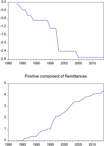
The non-linear ARDL is based on the assertion that a particular economic variable has different effect during positive and negative shock. Thus, the NARDL method divides remittances into positive and negative components. Figure 12 represents the negative and positive components of remittances.

Figure 12. Negative and Positive components of Remittances.

The lags and model specification of the NARDL model is presented in Table 2. Accordingly, the NARDL specification having lags 2, 2, 0 are selected based on the AIC criterion. The estimated long run and short run coefficients of NARDL are depicted in Table 3.

Table 2. Optimal lag and model selection criteria.

Model	AIC*	BIC	HQ	Adj. R-sq	Specification
8	−5.7984689	−5.464653	−5.691326	0.997251	ARDL(2, 2, 0)
4	−5.780946	−5.780946	−5.662817	0.997275	ARDL(2, 3,0)
7	−5.728344	−4.351159	−5.610215	0.9972127	ARDL(2. 2, 1)
3	−5.7166231	−5.291898	−5.583335	0.9971151	ARDL (2, 3, 1)

* shows an optimum selection of lag order.

Table 3. Results of non-linear ARDL equation.

Variable	Short run Coefficient	Std. Error	t-Statistic
LC(-1)	−0.173453***	0.308414	−3.630849
${\mathit{REM}}^{+}$ (-1)	0.042583***	0.014365	2.964463
${\mathit{REM}}^{-}$	0.028226***	0.014294	1.974589
D(LC(-1))	0.572122***	0.143800	3.978599
D(${\mathit{REM}}^{+}$ )	0.007791	0.014715	0.529469
D(${\mathit{REM}}^{-}$ (-1))	−0.036656	0.0147514	−2.266737
ECT(-1)	−0.173543***	0.041084	−4.224118
Variable	Long run Coefficient	Std. Error	t-Statistic
${\mathit{REM}}^{+}$	0.245377***	0.035720	6.869424
${\mathit{REM}}^{-}$	0.162644***	0.059238	2.745617
C	6.452614***	0.050902	126.7653
NARDL Bound test
$\mathrm{F}-\mathrm{statistic}\mathrm{ }\left(\mathrm{HYP}1\right)=\mathrm{ }3.946085\mathrm{ }[\mathrm{LB}=2.63,\mathrm{ }\mathrm{UB}=3.53\text{ at }10\mathrm{\%}]$ $\mathrm{ }[\mathrm{LB}=3.1,\mathrm{ }\mathrm{UB}=3.87\text{ at }5\mathrm{\%}]$

Note: ^{** *}depict significance at 1%.

The hypothesis regarding no long-run relationship between variables is rejected at one percent level of significance. Thus, there exists a long run relationship between remittances and CO2 emissions. The coefficients of long-run specify that the effect of positive variation in remittances (${\mathit{REM}}_t^{+}$ ) is nearly 0.25% and statistically significant at the 1% level. But on the other hand, the coefficient of remittance (${\mathit{REM}}_t^{-}$ ) is nearly 0.16% and also significant at one percent level. The effect of the negative component of remittance is less than the effect of positive component of remittances.

The presence of cointegration associations between the variables entails the estimation of the Error Correction Model (ECM) to understand the short-run relationships between variables in the model. The coefficient of ECM also shows the speed of adjustment to equilibrium when an economic shock is faced by an economy. The results of short-run coefficients and error correction term are reported in Table 3.

After a temporary shock, estimated short-run coefficients depict the conjunction to equilibrium in the long run. Keeping the views of econometric theory, the dynamic steadiness of the path of CO2 emissions needs that the parameter on the ECT must be negative and significant on the statistical background. As in our estimated model, the coefficient of error correction term is negative and also statistically significant at the level of 1% significance.

The estimated coefficient of the ECM is 17%. This reveals that the nearly 17% of disequilibrium in the preceding year following shocks to the system converge back to the long run equilibrium in the current year. By this ruling, it is deduced that to some extent disequilibrium within the CO2 emissions in the short run is hastily corrected and converged back to equilibrium in the long run.

To confirm the existence of long-run asymmetric association between remittances and CO2 emissions, we utilised the Wald test. The long run finding in Table 3 signifies that the negative and positive components of remittances are not the same, which depict an asymmetric association between remittances and CO2 emissions. The Wald test is reported in Table 4. The results of the Wald test depicted that there exists an asymmetrical association between remittances and CO2 emissions.

Table 4. Testing hypothesis of asymmetrical effect.

Null Hypothesis	F-Statistic	Probability
Long Run Symmetries (HYP2)	5.0503	0.033
Short Run Symmetries (HYP3)	6.5541	0.0165

To assess the adjustment of asymmetry in the existing long-run quilibrium after passing to a new long-run equilibrium due to negative and positive shocks, a dynamic multiplier graph is plotted for NARDL as shown in Figure 13. Here, the asymmetry curves show the linear mixture of the dynamic multipliers due to positive and negative remittances shocks.

Figure 13. NARDL Dynamic Multiplier Graph.

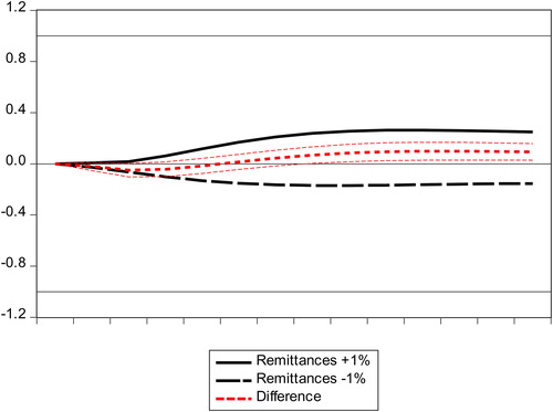
Figure 14. CUSUM Test.

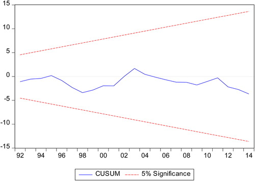
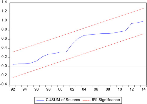
Figure 15. CUSUM of Square Test.

Positive and negative change curves indicate the evidence about the asymmetric adjustment of CO₂ emissions to negative and positive remittances shocks at a given period.

The difference between the positive component and negative component curve of remittances represents an asymmetry curve, which indicates the linear mixture of the dynamic multipliers linked with positive and negative remittances shocks. The positive change curve gives information about the asymmetric adjustment of CO2 emissions to positive remittances shock at a given forecasting horizon, while the negative variation curve gives knowledge about the asymmetric adjustment of CO2 emissions to negative remittances shock at a forecasting horizon. The overall intuition is that positive remittances shocks have a more deep impact on CO2 emissions in the long run comparedto the negative remittances shocks.

We carry out some diagnostic tests to validate our estimated results. These tests include the Jarque-Bera test which is used for checking normality in an estimated model, LM test which is used for identifying the problem of Autocorrelation, a White test which is used for detecting the problem of Heteroscedasticity, Ramsey Reset test which is applicable for checking the model for stability, CUSUM, and CUSUM of Square test. The results of these diagnostic tests reported in Table 5 show that our estimated model is free of any statistical problems.

Table 5. Validation test.

Test	Test-Statistic	Probability
Normality Test	1.183440	0.553375
LM Test	1.890423	0.3886
White test	27.49186	0.3318
Ramsay Reset test	2.709920	0.1633

Both CUSUM and CUSUM of Square tests confirm the stability of the estimated model (See Figure 14 & 15).

5. Conclusions

This paper attempts to develop a new theoretical framework that explains how the inflow of remittances causes a rise in carbon emissions. The theory is based on the assumption that the inflows of remittances affect CO2 emissions positively. Furthermore, we assumed that the inflows of remittances do not affect CO2 emissions directly rather than they affect carbon emissions indirectly through five different stages. After constructed theoretical framework, we tested the effect of remittances inflow on CO2 emissions. The selection of the NARDL model is based on the fact that macroeconomic variables rely on different economic conditions and that is why there exists a non-linear relationship among different macroeconomic variables. The ADF-GLS and PP unit root tests are employed to check the variables for tracking the order of integrations. The results of both unit root tests revealed that all the variables are I (1). The NARDL bound test shows that there exists a long run association between remittances and CO2 emissions. The Wald test confirmed that there exists an asymmetric linkage between remittances and CO2 emissions in both the short run and the long run. The findings also inferred that the effects of a positive component of remittances are more than the effect of negative component of remittances on CO2 emissions.

As remittances are an essential factor of financial development and economic growth, their role in polluting the environment cannot be denied. The current study recommends that the government should channel remittances for effective usage and more importantly should focus on sustainable and environmentally friendly financial expansion to avoid the adverse effect of remittances inflow on carbon emissions. Besides, remittances are considered one of the important factors of financial development. Thus, government should formulate lending policy in such a way that the banking sector or other financial institutions should lend money to those industries that follow the environmentally friendly production techniques. Thus, in this way the negative effect of remittances can be reduced. Moreover, government should encourage the financial sectors in order to invest in renewable energy resources so that dependency on harmful sources of energy will be reduced. One of the most important benefits of renewable energy is that it does not emit dangerous gases. In addition to this, a renewable source of energy is costlier. Therefore, it is imperative to allocate more money for research and development purposes to innovate the less costly source of energy for the protection of the environment.

6. Limitation and future research direction

The current study is limited to China; similar studies can be extended to other developing countries, especially by using more updated data and in the case of different cross-sections or countries including India, Pakistan, Sri-Lanka, Bangladesh and Nepal which receive a major portion of remittances.

References

- Alsamara, M., Mrabet, Z., Dombrecht, M., & Barkat, K. (2017). Asymmetric responses of money demand to oil price shocks in Saudi Arabia: A non-linear ARDL. Applied Economics, 49(37), 3758–3769. doi: 10.1080/00036846.2016.1267849
- Ang, J. B. (2008). Financial development and economic growth in Malaysia. London: Routledge.
- Arnold, R. A. (2008). Macroeconomics. Boston: Cengage Learning.
- Ayeche, M. B., Barhoumi, M., & Amin, M. (2016). Causal linkage between economic growth, financial development, trade openness and CO2 emissions in European Countries. American Journal of Environmental Engineering, 6, 110–122.
- Bagnai, A., & Ospina, C. A. (2016). Asymmetric asymmetries” in Eurozone markets gasoline pricing. The Journal of Economic Asymmetries, 13, 89–99. doi: 10.1016/j.jeca.2016.03.004
- Balde, Y. (2011). The Impact of Remittances and Foreign Aid on Savings/Investment in Sub-Saharan Africa. African Development Review, 23, 247–262.
- Başarir, Ç., & Çakir, Y. N. (2015). Causal Interactions between Co2 emissions, financial development, energy and tourism. Asian Economic and Financial Review, 26, 1227–1238.
- Bhole. (2009). Financial institutions & markets 5E. New York: Tata McGraw-Hill Education.
- Boutabba, M. A. (2014). The impact of financial development, income, energy and trade on carbon emissions: Evidence from the Indian economy. Economic Modelling, 40, 33–41. doi: 10.1016/j.econmod.2014.03.005
- Caporale, G., & Pittis, N. (1999). Efficient estimation of cointegration vectors and testing for causality in vector autoregressions. J. Econ. survey, 13, 1–35. doi: 10.1111/1467-6419.00073
- Chang, M. I. (2011). Pollution in China: China in the 21st century. New York: Nova Science Publishers.
- Chow, G. C. (2015). China’s Economic Transformation. Wiley.
- Corsepius, U. (1989). Peru at the brink of economic collapse: Current problems and policy options. Germany: Institut für Weltwirtschaft.
- de Bruyn, S. M., van den Bergh, J. C. J. M., & Opschoor, J. B. (1998). Economic growth and emissions: Reconsidering the empirical basis of Environmental Kuznets curves. Ecological Economics, 25(2), 161–175. doi: 10.1016/S0921-8009(97)00178-X
- Dickey, D., & Fuller, W. (1979). Distribution of the estimator for autoregressive time series with a unit root. Journal of American Statistical Association, 74, 427–431. doi: 10.1080/01621459.1979.10482531
- Dinda, S. (2004). Environmental Kuznets curve hypothesis: A survey. Ecological Economics, 49(4), 431–455. doi: 10.1016/j.ecolecon.2004.02.011
- Elafif, M., Alsamara, M. K., Mrabet, Z., & Gangopadhyay, P. (2017). The asymmetric effects of oil price on economic growth in Turkey and Saudi Arabia: New evidence from nonlinear ARDL approach. International Journal of Development and Conflict, 7, 97–118.
- Elliott, G., Rothenberg, T., & Stock, J. (1996). Efficient tests for an autoregressive unit root. Econometrica, 64(4), 813–836. doi: 10.2307/2171846
- Farhani, S., & Ozturk, I. (2015). Causal relationship between CO2 emissions, real GDP, energy consumption, financial development, trade openness, and urbanization in Tunisia. Environmental Science and Pollution Research, 22(20), 15663. doi: 10.1007/s11356-015-4767-1
- Friedl, B., & Getzner, M. (2003). Determinants of CO2 emissions in a small open economy. Ecological Economics, 45(1), 133–148. doi: 10.1016/S0921-8009(03)00008-9
- Granger, C., & Yoon, G. (2002). Hidden cointegration. Working paper, UCSD.
- Graziani, A. (2003). The monetary theory of production. Cambridge: Cambridge University Press.
- Grossman, G., & Krueger, A. (1995). Economic environment and the economic growth. Quarterly Journal of Economics, 110(2), 353–377. doi: 10.2307/2118443
- Hahnel, R. (1999). Panic rules!: Everything you need to know about the global economy. Boston: South End Press.
- Heil, M., & Selden, M. (2001). Carbon emissions and economic development: Future trajectories based on historical experience. Environment and Development Economics, 6 (1), 63–83. doi: 10.1017/S1355770X01000043
- Herendeen, J. B. (2007). Issues in economics: An introduction. USA: University Press of America.
- Herr, H., & Kazandziska, M. (2011). Macroeconomic policy regimes in western industrial countries. London: Routledge.
- Hijazi, M. H. (2016). he giving world: The three financial forces that could transform global development. Oxford: Infinite Ideas.
- Holtz-Eakin, D., & Selden, T. (1995). Stoking the fires? CO2 emissions and economic growth. Journal of Public Economics, 57(1), 85–101. doi: 10.1016/0047-2727(94)01449-X
- Iheke, O. (2012). The effect of remittances on the Nigerian economy. International Journal of Development and Sustainability, 1, 614–621.
- Jamel, L., & Maktouf, S. (2017). The nexus between economic growth, financial development, trade openness, and CO2 emissions in European countries. Cognet Economics & Finance, 5.
- Kedourie, E. (2013). The Middle Eastern Economy: Studies in economics and economic history. London: Routledge.
- Lakhera, M. (2016). Economic growth in developing countries: Structural transformation, manufacturing and transport infrastructure. New York: Springer.
- Li, S., Zhang, J., & Ma, Y. (2015). Financial development, environmental quality and economic growth. Sustainability, 7(7), 9395–9416. doi: 10.3390/su7079395
- Liu, Z. (2016). Carbon emissions in China. New York: Springer.
- Malinvaud, E. (1979). Economic growth and resources. New York: Springer.
- Mamun, M. A., Sohag, K., Samargandi, N. & Farid, (2016). Does remittance fuel labour productivity in Bangladesh? The application of an asymmetric non-linear ARDL approach. Applied Economics, 48, 4861–4877.
- Managi, S., & Jena, P. (2008). Environmental productivity and Kuznets curve in India. Ecological Economics, 65(2), 432–440. doi: 10.1016/j.ecolecon.2007.07.011
- Meyer, D., & Shera, A. (2017). The impact of remittances on economic growth: An econometric model. EconomiA, 18(2), 147–155. doi: 10.1016/j.econ.2016.06.001
- Moomaw, W., & Unruh, G. (1997). Are environmental Kuznets curve misleading us? The case of CO 2 emissions. Environment and Development Economics, 2, (4), 451–463. doi: 10.1017/S1355770X97000247
- Motelle, S. I. (2011). The role of remittances in financial development in Lesotho: Evidence from alternative measures of financial development. Journal of Development and Agricultural Economics, 241–251.
- Mugableh, M. I. (2015). Economic Growth, CO 2 Emissions, and Financial Development in Jordan: Equilibrium and Dynamic Causality Analysis. International Journal of Economics and Finance, 98–105. doi: 10.5539/ijef.v7n7p98
- Mulali, U. A., Tang, C. F., & Oztur, I. (2015). Does financial development reduce environmental degradation? Evidence from a panel study of 129 countries. Environmental Science and Pollution Research, 22, 14891–14900. doi: 10.1007/s11356-015-4726-x
- Nusair, S. A. (2016). The effects of oil price shocks on the economies of the Gulf Co-operation Council countries: Nonlinear analysis. Energy Policy, 91(C), 256–267. doi: 10.1016/j.enpol.2016.01.013
- Obradovic, S., & Lojanica, N. (2017). Energy use, CO2 emissions and economic growth– causality on a sample of SEE countries. Economic Research-Ekonomska Istraživanja, 30(1), 511–526. doi: 10.1080/1331677X.2017.1305785
- Ozturk, I., & Acaravci, A. (2013). The long-run and causal analysis of energy, growth, openness and financial development on carbon emissions in Turkey. Energy Economics, 36, 262–267. doi: 10.1016/j.eneco.2012.08.025
- Ozturk, I., & Uddin, G. S. (2012). Causality among carbon emissions, energy consumption and growth in India. Economic Research-Ekonomska Istraživanja, 25(3), 752–775. doi: 10.1080/1331677X.2012.11517532
- Pacala, S., & Socolow, R. (2004). Stabilization wedges: Solving the climate problem for the next 50 years with current technologies. Science, 305(5686), 968–972. doi: 10.1126/science.1100103
- Pal, D., & Mitra, S. K. (2015). Asymmetric impact of crude price on oil product pricing in the United States: An application of multiple threshold nonlinear autoregressive distributed lag model. Economic Modelling, 51, 436–443. doi: 10.1016/j.econmod.2015.08.026
- Pal, D., & Mitra, S. K. (2016). Asymmetric oil product pricing in India: Evidence from a multiple threshold nonlinear ARDL model. Economic Modelling, 59, 314–328. doi: 10.1016/j.econmod.2016.08.003
- Pesaran, M. H., Shin, Y., & Smith, R. J. (2001). Bounds testing approaches to the analysis of level relationships. Journal of Applied Econometrics, 16(3), 289–326. doi: 10.1002/jae.616
- Pesaran, M., & Shin, Y. (1998). An autoregressive distributed-lag modelling approach to cointegration analysis. Econometric Society Monographs, 31, 371–413.
- Pesaran, M., & Shin, Y. (1999). An autoregressive distributed lag modelling approach to cointegration analysis’ In. S Strom, (ed.). Econometrics and economic theory in the 20th century: the Ragnar Frisch centennial symposium. Cambridge: Cambridge U P.
- Pesaran, M., Shin, Y., & Smith, R. (2001). Bonds testing approaches to the analysis of level relationship. Journal of Applied Econometrics, 16(3), 289–326. doi: 10.1002/jae.616
- Phillips, P., & Perron, P. (1988). Testing for unit root in time series regression. Biometrica, 75(2), 335–346. doi: 10.2307/2336182
- Prabal, K. D., & Dilip, R. (2012). Impact of remittances on household income, asset and human capital: Evidence from Sri Lanka. Migration and Development, 1(1), 163–179. doi: 10.1080/21632324.2012.719348
- Saboori, B., Sulaiman, J., & Mohd, S. (2012). Economic growth and CO2 emissions in Malaysia: A cointegration analysis of the Environmental Kuznets Curve. Energy Policy, 15, 184–191. doi: 10.1016/j.enpol.2012.08.065
- Saidi, K., & Mbarek, M. B. (2017). The impact of income, trade, urbanization, and financial development on CO 2 emissions in 19 emerging economies. Environmental Science and Pollution Research, 24(14), 12748–12757. doi: 10.1007/s11356-016-6303-3
- Salisu, A. A., & Isah, K. O. (2017). Revisiting the oil price and stock market nexus: A nonlinear Panel ARDL approach. Economic Modelling, 66, 258–271. doi: 10.1016/j.econmod.2017.07.010
- Sawyer, W. C., & Sprinkle, R. L. (2015). Applied international economics. London: Routledge.
- Schorderet, Y. (2001). Revisiting Okun' s law: An hysteretic perspective. Mimeo, San Diego: University of California.
- Schorderet, Y. (2003). Asymmetric cointegration. Université de Genève/Faculté Des Sciences Économiques et Sociales.
- Selden, T. & Song, (1994). Environmental quality and development: Is there a Kuznets curve for air pollution?. Journal of Environmental Economics and Management, 147–162. doi: 10.1006/jeem.1994.1031
- Sentā, T. K. (1966). Postwar economic growth in Japan: Selected papers of the first conference of the Tokyo economic research center. California: University of California Press.
- Sexton, R. L. (2015). Exploring macroeconomics. Boston: Cengage Learning.
- Shin, h., Baek, J., & Heo, E. (2018). Do oil price changes have symmetric or asymmetric effects on Korea’s demand for imported crude oil?. Energy Sources, Part B: Economics, Planning, and Policy, 13(1), 6–12. doi: 10.1080/15567249.2017.1374489
- Shin, Y., Yu, B., & Greenwoo, M. (2013). Modelling asymmetric cointegration and dynamic multipliers in a nonlinear ARDL framework. New York: Springer.
- Shucheng, L. (2017). Chinese economic growth and fluctuations. New York: Taylor & Francis.
- Stern, D. (2004). The rise and fall of the environmental Kuznets curve. World Development, 32 (8), 1419–1439. doi: 10.1016/j.worlddev.2004.03.004
- Swanson, T., & Lin, T. (2009). Economic Growth and Environmental Regulation: China's Path to a Brighter Future. London: Routledge.
- Tregarthen, T. D., & Rittenberg, L. (1999). Macroeconomics, Second Edition. Macmillan.
- Tregarthen, T., & Rittenberg, L. (1999). Economics, Second Edition. Basingstoke: Macmillan.
- Tucker, I. (2008). Survey of economics. Boston: Cengage Learning.
- World Bank Group. (2017). Migration and remittances: Recent development and outlook. Washington: World Bank Group.
- Xing, T., Jiang, Q., & Ma, X. (2017). To facilitate or curb? The role of financial development in China’s carbon emissions reduction process: A novel approach. International Journal of Environmental Research and Public Health, 14(10), 1222. doi: 10.3390/ijerph14101222
- Zhang, Y. J. (2011). The impact of financial development on carbon emissions: An empirical analysis in China. Energy Policy, 39(4), 2197–2203.