Price rigidity, market competition, and product differentiation

Abstract

This study develops a two-period model in which the manufacturer determines a price floor and sets production output before demand becomes certain. The model defines the distance between price floor and high-demand-state price in concern to the degree of price flexibility. While conflicting empirical results underscore the importance of theoretical underpinnings, this study shows that economies of scale determine the relation between market competition and price rigidity. A decline in output leads to higher average costs in the industry characterised by economies of scale, a hike in average costs adds pressure on the inventory liquidation that drives price cutting in the low-demand state. Prices tend to more fluctuate as the product becomes more homogeneous or more players enter into the industry. The knowledge of the relationship between market competition, product homogeneity, and price rigidity is critical in formulating antitrust and monetary policies.

Keywords:

• price rigidity
• Cournot competition
• returns to scale

Subject Classification Codes:

• D21
• L11
• M21

1. Introduction

Across national boundaries and over time, changes in demand for goods have been accompanied by only a partial price-level response (Gordon, 1981). Studies of price rigidity have offered implications for various academic disciplines. For example, in marketing, pricing and price adjustment plays a critical role in a business determining how to adjust the prices of individual products in response to temporary cost increases, how to adjust prices to competitors’ price changes, and how to adjust the prices of sale and non-sale items. In the field of microeconomics, understanding the price change process can provide insights into issues such as the price rigidity of individual products, the rate at which costs are passed through to prices, and the time it takes prices to adjust to changes in market conditions (e.g., changes in supply and demand). Because price-setting behavior influences the way in which monetary policy affects the economy, central banks must understand how companies set prices. Understanding the extent of these nominal rigidities, their causes, and to what extent they react asymmetrically to demand or supply shocks is therefore crucial to formulate and implement monetary policy. According to Gordon (1981), understanding the reasons for the heterogeneity in price rigidity is crucial for the theory of price adjustment. Peltzman (2000) finds asymmetric price transmission to be the rule rather than the exception and the standard economic theory of markets remains incomplete. Meyer and Cramon-Taubadel (2004) indicate that sluggish price is not only important because it may point to gaps in economic theory, but also because its presence is often considered for policy purposes to be evidence of market failure.

Price rigidity variations refer to the high and low levels of nominal price inertia across product categories, firm sizes, and market structures (Carlton, 1986). Conlisk et al. (1984) develop a model to show that prices of durable goods remain constant for a length of time, drops temporarily and then returns to the initial level. According to the Tirole (1988), prices could be rigid because there are incentives for firms to sustain prices at higher levels through implicit agreements. Caucutt et al. (1999) document the extent of price rigidity across U.S. manufacturing industries and found that durable products have relatively high price rigidity across industrial product classes.

The existing empirical evidence reflects the ambiguity concerning the direction of the effect of industrial concentration on the rate of price adjustment. Several studies have found that the level of market concentration is strongly correlated with price stickiness (Carlton, 1986; Caucutt et al., 1999; Geroski, 1992). Carlton (1986) concludes that length of a spell of price rigidity is positively related to the four-firm concentration ratio. Geroski (1992) examines the data of U.K. manufacturing industries; the result suggests that pricing dynamics are more sluggish to shocks in more concentrated industries. Caucutt et al. (1999) use the U.S. Bureau of Labor Statistics (B.L.S.) individual-commodity monthly price series and finds price rigidity is positively related to four-firm concentration ratio. However, studies that have used aggregate data to examine the rate of price adjustment have yielded conflicting results. Domberger (1979, 1983) finds a positive relationship between the speed of price adjustment and Herfindahl index of concentration, his argument is communication on price information between firms facilitated by concentration. Domowitz et al. (1986) uses data from the U.S. Census of Manufacture and finds that price-cost margins in manufacturing are more procyclical in more concentrated industries. Setiawan et al. (2015) investigate the relationship between industrial concentration and price rigidity in the Indonesian market and suggest that industrial concentration has a positive effect on percentage price changes. The relationship between price rigidity and market structure remains an inconclusive issue in literature, the main difficulty in resolving the controversy is the lack of a clear-cut rationale explaining the phenomena.

The stipulation of a price floor is one of most commonly used practice in the industries. Butz (1997) creates a model in which the manufacturer employs resale price maintenance to restrict low-demand dealer rivalry. Minimum resale price maintenance is a widely used practice whereby an upstream entity specifies a minimum price to which a downstream entity is required to adhere. Butz (1997) assumes demand is binary distribution and price is binding if demand turns out low and manufacturer repurchases each retailer’s unsold inventories. Jullien and Rey (2007) conclude that a price floor in marketing channel leads to price rigidity that facilitates the detection of a deviation for a collusive agreement.

The remainder of this article is organised as follows. Section 2 presents a model in which a monopoly manufacturer treats output and the price floor as endogenous variables. This section also examines how salvage values, production costs, the length of production affect price rigidity. Section 3 introduces more players into the model and examines the effect of competition on price rigidity. Section 4 confirms product homogeneity in industries with economies of scale is positively related to price fluctuations. Finally, Section 5 explains the economic implications of these models and concludes.

2. Price floor model

In this section, we construct a model, in which there is a monopoly manufacturer and, in the subsequent section, competition is introduced by adding other players. The following basic assumptions are needed:

Assumption 1:

A two-period model in which the firm produces or purchases merchandise at $T=1$ and sells at $T=2$. At $T=1$, the current demand faced by the firm is given by: (1) $$P=(\mathit{aX}-Q)b^{-1},$$(1) where $a,b>0$ are constants, $Q$ is output, $P$ is market price, and $X$ is demand uncertainty, which becomes certain at $T=2$ and has the following binominal probability distribution (Chen, 2016): (2) $$X=\{\begin{array}{c}{X}_H=X{e}^{v\sqrt{t}},\mathit{withprobability}=\alpha \\ X_L=X{e}^{-v\sqrt{t}},\mathit{with}\mathit{probability}=1-\alpha \end{array}.$$(2)

The probability $\alpha >0$ can be given exogenously or determined endogenously. The latter is the risk-neutral probability (Cox et al., 1979), and this can be written as: (3) $$\alpha =\frac{e^{\mathit{rt}}-e^{-v\sqrt{t}}}{e^{v\sqrt{t}}-e^{-v\sqrt{t}}},$$(3) where $r>0$ denotes the discount rate, $v>0$ the volatility of demand shocks, and $t>0$ the length of the production period, while $e^{v\sqrt{t}}$ and $e^{-v\sqrt{t}}$ represent the percentages of upward and downward movements, respectively. The risk-neutral probability has the advantage of being independent of subjective beliefs regarding the occurrence of the possible states, which ensures that the expected growth rate of demand equals the discount rate $r$, which can be written as: (4) $$e^{\mathit{rt}}=\alpha \cdot e^{v\sqrt{t}}+(1-\alpha )e^{-v\sqrt{t}}.$$(4)

Equation (4)(4) $$e^{\mathit{rt}}=\alpha \cdot e^{v\sqrt{t}}+(1-\alpha )e^{-v\sqrt{t}}.$$(4) shows that once the appropriate discount rate is chosen, the expected growth rate of demand is independent of volatility and probability. It must be noted that the choice of probability determination will not influence any result in this study.

Assumption 2:

For a two-period model under demand uncertainty, the manufacturer must determine its production output before demand becomes certain. At $T=1$, the manufacturer produces a cost function as follows: (5) $$\mathit{TC}=(f_0+f_{1}Q)Q,$$(5)

Where $f_0>0$ is a constant, it is important to specify the minimum value of $f_1$: (6) $$f_1>-\frac{\alpha e^{-\mathit{rt}}}{b}.$$(6)

Inequality (6) ensures the existence of optimal solution for the firm maximising its profits. Although Inequality (6) allows the case of economies of scale (i.e., unit cost is a decreasing function of output) with $f_1<0$, it requires that $f_1$ cannot be too low otherwise the profit maximisation solution cannot be defined.

Assumption 3:

Along with production output $Q$, the manufacturer determines price floor $\underset{\_}{\mathit{P}}$ before market demand becomes certain. If the low-demand state ($X=X_L$) occurs and the market-clearing price is below the price floor at $T=2$, there are unsold quantities at the binding price floor, and the salvage value per unit of unsold goods is $s$. To rule out the arbitrage opportunity, we restricted $s<a{X}_L/b$. Without this restriction, firms will not sell products in consumer markets when $X=X_L$, and if $s$ is higher than market prices when $X=X_H$ then the second order condition for maximum profits will not exist.

Given these three assumptions, the profit maximisation problem for the monopoly manufacturer can now be defined as: $$\begin{array}{l}\underset{Q,\underset{\_}{\mathit{P}}}{\overset{}{\mathit{Max}}}\begin{array}{c}\end{array}{\pi }_M=(-f_0-f_{1}Q)Q+m(\frac{a}{b}{X}_H-\frac{Q}{b})Q+u\underset{\_}{\mathit{P}}(a{X}_L-b\underset{\_}{\mathit{P}})+\mathit{us}(Q-(a{X}_L-b\underset{\_}{\mathit{P}}))\\ \begin{array}{ll}s.t.& \end{array}\frac{a{X}_H}{b}-\frac{Q}{b}\ge \underset{\_}{\mathit{P}}\ge \frac{a{X}_L}{b}-\frac{Q}{b}\end{array}$$ where $m=\alpha e^{-\mathit{rt}}$ and $u=(1-\alpha )e^{-\mathit{rt}}$ for simplicity. If the constraint $\frac{a{X}_H}{b}-\frac{Q}{b}\ge \underset{\_}{\mathit{P}}$ were to be violated, goods would not be fully sold, even in the high-demand state. This would be economically unreasonable and the second-order sufficient conditions for profit maximisation would not hold. If the constraint $\underset{\_}{\mathit{P}}\ge \frac{a{X}_L}{b}-\frac{Q}{b}$ were to be violated, the price floor would not bind even in the low-demand state, rendering the price floor meaningless. The solution to output and price floor can be found by forming the Lagrangian and satisfying the Kuhn–Tucker conditions (Chen, 2016): (7) $$\mathcal{L}=\left(-f_0-f_{1}Q\right)Q+m(\frac{a}{b}{X}_H-\frac{Q}{b})Q+u\underset{¯}{\mathit{P}}(a{X}_L-b\underset{¯}{\mathit{P}})+\mathit{us}(Q-(a{X}_L-b\underset{¯}{\mathit{P}}))+{\lambda }_1(\frac{a{X}_H}{b}-\frac{Q}{b}-\underset{¯}{\mathit{P}})+{\lambda }_2(\underset{¯}{\mathit{P}}-\frac{a{X}_L}{b}+\frac{Q}{b}).$$(7)

The Kuhn–Tucker conditions are as follows: $$\begin{array}{c}\frac{\partial \mathcal{L}}{\partial Q}\le 0\begin{array}{cc}& \end{array}\begin{array}{c}\end{array}Q\ge 0\begin{array}{cc}& \end{array}Q\frac{\partial \mathcal{L}}{\partial Q}=0,\\ \frac{\partial \mathcal{L}}{\partial \underset{\_}{\mathit{P}}}\le 0\begin{array}{cc}& \end{array}\begin{array}{c}\end{array}\underset{\_}{\mathit{P}}\ge 0\begin{array}{c}\begin{array}{c}\end{array}\end{array}\begin{array}{c}\end{array}\begin{array}{c}\end{array}\begin{array}{c}\end{array}\underset{\_}{\mathit{P}}\frac{\partial \mathcal{L}}{\partial \underset{\_}{\mathit{P}}}=0,\\ \frac{\partial \mathcal{L}}{\partial {\lambda }_1}\le 0\begin{array}{cc}& \end{array}{\lambda }_1\ge 0\begin{array}{cc}& \end{array}{\lambda }_1\frac{\partial \mathcal{L}}{\partial {\lambda }_1}=0,\\ \frac{\partial \mathcal{L}}{\partial {\lambda }_2}\le 0\begin{array}{cc}& \end{array}{\lambda }_2\ge 0\begin{array}{cc}& \end{array}{\lambda }_2\frac{\partial \mathcal{L}}{\partial {\lambda }_2}=0.\end{array}$$

Lemma 1:

Given Assumptions 1–3, the manufacturer’s optimal strategy consists of setting its production output and price floor according to various constraints: (8) $$\begin{array}{c}Q=\frac{\mathit{am}{X}_H+\mathit{bus}-b{f}_0}{2f_{1}b+2m},\underset{\_}{\mathit{P}}=\frac{a{X}_L}{2b}+\frac{s}{2}\text{if}\frac{a{X}_H}{b}-\frac{Q}{b}>\underset{\_}{\mathit{P}}>\frac{a{X}_L}{b}-\frac{Q}{b}\text{or}\\ \frac{4\mathit{ab}{f}_1{X}_L-2am{X}_H+4\mathit{am}{X}_L+2b{f}_0}{b(2f_{1}b+2m+2u)}<s<\frac{4ab{X}_H{f}_1-2f_{1}ab{X}_L+2am(X_H-X_L)+2b{f}_0}{b(2f_{1}b+2m+2u)},\end{array}$$(8) $$\begin{array}{c}Q=\frac{a{X}_H{e}^{-\mathit{rt}}+\mathit{au}(X_H-X_L)-b{f}_0}{2f_{1}b+2e^{-\mathit{rt}}}\\ \text{if}\underset{\_}{\mathit{P}}=\frac{a{X}_H}{b}-\frac{Q}{b}\text{or}\frac{4ab{X}_H{f}_1-2f_{1}ab{X}_L+2am(X_H-X_L)+2b{f}_0}{b(2f_{1}b+2m+2u)}\le s<\frac{a{X}_L}{b},\end{array}$$ (10) $$\begin{array}{c}Q=\frac{\mathit{am}{X}_H+\mathit{au}{X}_L-b{f}_0}{2f_{1}b+2e^{-\mathit{rt}}}\\ \text{if}\underset{\_}{\mathit{P}}=\frac{a{X}_L}{b}-\frac{Q}{b}\text{or}s\le \frac{4\mathit{ab}{f}_1{X}_L-2am{X}_H+4\mathit{am}{X}_L+2b{f}_0}{b(2f_{1}b+2m+2u)}.\end{array}$$(10)

Proof:

Please see Appendix.

Equations (8)–(10) enable us to assess the position of the price floor relative to the prices in the high- and low-demand states, denoted by $P_H=a{X}_H/b-Q/b$ and $P_L=a{X}_L/b-Q/b$, respectively. A high degree of price rigidity corresponds to the price floor being near the price in the high-demand state, whereas prices are entirely flexible when the price floor coincides with the price in the low-demand state.

Proposition 1:

When$\frac{4\mathit{ab}{f}_1{X}_L-2am{X}_H+4\mathit{am}{X}_L+2b{f}_0}{b(2f_{1}b+2m+2u)}<s<\frac{4ab{X}_H{f}_1-2f_{1}ab{X}_L+2am(X_H-X_L)+2b{f}_0}{b(2f_{1}b+2m+2u)}$ or $\frac{a{X}_H}{b}-\frac{Q}{b}>\underset{\_}{\mathit{P}}>\frac{a{X}_L}{b}-\frac{Q}{b}$, the degree of price flexibility increases with a lower salvage value $s$, higher cost parameters $f_0,f_1$.

Proof:

Please see Appendix.

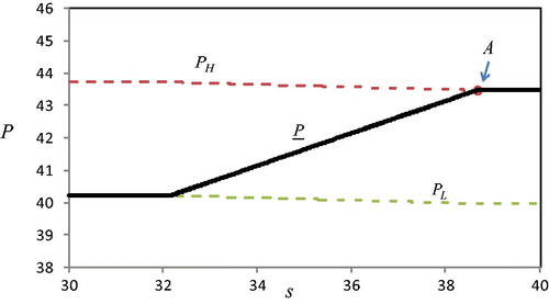
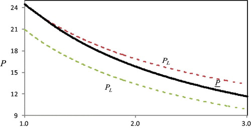
Figure 1 represents that how the durability affects the degree of price rigidity in the selling season. As salvage value $s$ increases, price floor $\underset{\_}{\mathit{P}}$ rises until it reaches the price in the high-demand state. At a point $A$, the price floor coincides with the price in the high-demand state; however, the market price is fixed regardless of demand fluctuations and thus it demonstrates perfect rigidity. Because the high salvage value, or the long shelf-life, limits the downside risk, the producer does not have to cut prices to generate sales. This result corresponds with those of Conlisk et al. (1984) and Caucutt et al. (1999), who found that durable products have relatively high price rigidity across industrial product classes. Consistently, Serra and Goodwin (2003) also demonstrated that the prices of highly perishable dairy products in Spain are flexible.

Figure 1. Salvage value and price rigidity.

Parameter values:$a=50,b=1,X=1,v=0.035,r=0.02,f_0=2,f_1=2$

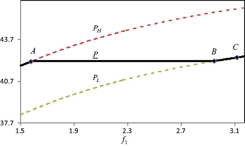
As similarly indicated by Proposition 1, Figure 2 shows that the magnitude of price changes becomes greater as the parameters of unit cost $f_1$ increases. The economic intuition behind Figure 2 is, as unit cost rises over salvage value, the pressure of unsold goods increases accordingly, therefore the distance between high-demand price and price floor widens. The greater distance creates an asymmetric price adjustment in response to cost changes during the low-demand period. From point $B$ to point $C$, the market price increases with a rise in the production cost; however, from point $B$ to point $A$, the production cost decreases but the market price remains unchanged. The illustration that prices rise faster, following positive cost shocks than they fall as costs decline is consistent with the findings of Peltzman (2000) and Setiawan et al. (2015). However, when demand is in the high-state, the adjustments of market price $P_H$ to upward and downward cost changes are symmetric. The price unresponsiveness to cost changes is likely to take place in the low-demand state, a finding that corresponds with that of Kraft (1995), who used German data to show that prices are more rigid to cost shocks during periods of recession than in boom times. If firms with high capital intensity is characterised by a low value of $f_1$, our model predicts a positive effect of capital intensity on price rigidity, consistent with the works of Schramm and Sherman (1977), Kraft (1995), and Weiss (1995). A large firm tends to experience economies of scale where output rises faster than the cost, so a large firm is more likely to have a low value of $f_1$. Greenslade and Parker (2012) showed that larger firms reviewed their prices more often than smaller firms, and set prices according to economic conditions.

Figure 2. Production cost and price rigidity.

Parameter values:$a=50,b=1,X=1,v=0.035,r=0.02,f_0=2,s=36$

3. Market competition

The effect of market competition on price rigidity plays an essential role in formulating antitrust and economic policies. By modifying the assumption of a monopoly manufacturer to $n$ homogeneous manufacturers, Equation (1)(1) $$P=(\mathit{aX}-Q)b^{-1},$$(1) can be rewritten as: (1) $$P=\frac{\mathit{aX}}{b}-\frac{(q_1+q_2+\dots q_n)}{b}.$$(1)

The profit maximisation problem of an individual manufacturer,${\pi }_i,i=1..n$, can be described as: (20) $$\begin{array}{c}\underset{q_i,\underset{\_}{P_i}}{\mathit{Max}}\begin{array}{c}\end{array}{\pi }_i=\left(-f_0-f_{1}q{}_i\right)q_i+m(\frac{a}{b}{X}_H-\frac{Q}{b})q_i+u{\underset{\_}{\mathit{P}}}_i(a{X}_L-Q_{-i}-b{\underset{\_}{\mathit{p}}}_i)+\mathit{us}(q_i-(a{X}_L-Q_{-i}-b{\underset{\_}{\mathit{p}}}_i))\\ \begin{array}{cc}s.t.& \end{array}\frac{a{X}_H}{b}-\frac{Q}{b}\ge {\underset{\_}{\mathit{p}}}_i\ge \frac{a{X}_L}{b}-\frac{Q}{b},\end{array}$$(20)

Where $Q$ is the combined output of all firms and $Q_{-i}=Q-q_i$ is the combined output of all firms except $i$. If player $i$ in the Cournot game chose its output $q_i$ and price floor ${\underset{\_}{\mathit{p}}}_i$, the solution to Equation (20)(20) $$\begin{array}{c}\underset{q_i,\underset{\_}{P_i}}{\mathit{Max}}\begin{array}{c}\end{array}{\pi }_i=\left(-f_0-f_{1}q{}_i\right)q_i+m(\frac{a}{b}{X}_H-\frac{Q}{b})q_i+u{\underset{\_}{\mathit{P}}}_i(a{X}_L-Q_{-i}-b{\underset{\_}{\mathit{p}}}_i)+\mathit{us}(q_i-(a{X}_L-Q_{-i}-b{\underset{\_}{\mathit{p}}}_i))\\ \begin{array}{cc}s.t.& \end{array}\frac{a{X}_H}{b}-\frac{Q}{b}\ge {\underset{\_}{\mathit{p}}}_i\ge \frac{a{X}_L}{b}-\frac{Q}{b},\end{array}$$(20) would be found by forming the Lagrangian: (21) $$\begin{array}{c}\mathcal{L}=\left(-f_0-f_{1}q{}_i\right)q_i+m(\frac{a}{b}{X}_H-\frac{Q}{b})q_i+u{\underset{¯}{\mathit{P}}}_i(a{X}_L-Q_{-i}-b{\underset{¯}{\mathit{p}}}_i)+\mathit{us}(Q-(a{X}_L-Q_{-i}-b{\underset{¯}{\mathit{p}}}_i))\\ \begin{array}{c}\end{array}+{\lambda }_1(\frac{a{X}_H}{b}-\frac{Q}{b}-{\underset{¯}{\mathit{p}}}_i)+{\lambda }_2({\underset{¯}{\mathit{p}}}_i-\frac{a{X}_L}{b}+\frac{Q}{b}).\end{array}$$(21)

Lemma 2:

Suppose that Assumptions 1–3 hold and that $n$ manufacturers engage in Cournot competition; hence, each manufacturer’s optimal strategy consists of setting production output $q_i$ and price floor ${\underset{\_}{\mathit{p}}}_i$,$i=1..n$, as follows: $$q_i=\frac{\mathit{am}{X}_H+\mathit{bus}-b{f}_0}{2f_{1}b+(n+1)m},\begin{array}{c}\end{array}{\underset{\_}{\mathit{p}}}_i=\frac{a{X}_L}{2b}+\frac{s}{2}-\frac{(n-1)(\mathit{am}{X}_H+\mathit{bus}-b{f}_0)}{2b(2f_{1}b+(n+1)m)}$$ (22) $$\text{If}\frac{2\mathit{ab}{f}_1{X}_L+\mathit{am}(n+1)(X_L-X_L)+b(n+1)f_0}{b(2f_{1}b+(+(n+1)m+(n+1)u)}<s<\frac{4ab{X}_H{f}_1-2f_{1}ab{X}_L+\mathit{am}(n+1)(X_H-X_L)+b(n+1)f_0}{b(2f_{1}b+(+(n+1)m+(n+1)u)},$$(22) (23) $$q_i=\frac{a{X}_H{e}^{-\mathit{rt}}+\mathit{au}(X_H-X_L)-b{f}_0}{2f_{1}b+(n+1)e^{-\mathit{rt}}}\text{if}\frac{4ab{X}_H{f}_1-2f_{1}ab{X}_L+\mathit{am}(n+1)(X_H-X_L)+b(n+1)f_0}{b(2f_{1}b+(+(n+1)m+(n+1)u)}\le s<\frac{a{X}_L}{b},$$(23) (24) $$q_i=\frac{\mathit{am}{X}_H+\mathit{au}{X}_L-b{f}_0}{2f_{1}b+(n+1)e^{-\mathit{rt}}}\text{if}s\le \frac{2\mathit{ab}{f}_1{X}_L+\mathit{am}(n+1)(X_L-X_L)+b(n+1)f_0}{b(2f_{1}b+(+(n+1)m+(n+1)u)}.$$(24)

Proof:

Please see Appendix.

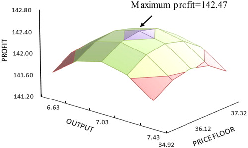
As taking rival’s output as fixed, each firm is making the best response to each other. The output $q_i$ and ${\underset{\_}{\mathit{p}}}_i$ derived in Lemma 2 are an equilibrium that maximises profit, it is no incentive for firms to deviate. Table 1 and Figure 3 used a numerical example to illustrate that no firm will cut the price by lowering price floor in equilibrium. Suppose that there are two firms, the parameter values are as follows:$a=50,b=1,X=1,v=0.035,r=0.02,f_0=2,f_1=2,s=31$, then two firms will choose $q_1=q_2=7.03$, ${\underset{\_}{\mathit{p}}}_1={\underset{\_}{\mathit{p}}}_2=36.12$ based on the Equation (22)(22) $$\text{If}\frac{2\mathit{ab}{f}_1{X}_L+\mathit{am}(n+1)(X_L-X_L)+b(n+1)f_0}{b(2f_{1}b+(+(n+1)m+(n+1)u)}<s<\frac{4ab{X}_H{f}_1-2f_{1}ab{X}_L+\mathit{am}(n+1)(X_H-X_L)+b(n+1)f_0}{b(2f_{1}b+(+(n+1)m+(n+1)u)},$$(22) . Given firm 2 output is fixed, firm 1 has no incentive to deviate current choices, because other combinations of $q_i$ and ${\underset{\_}{\mathit{p}}}_i$ generate lower profit than that in equilibrium.

Table 1. Firm’s profit under different combinations of output and price floor, given competing for opponent choices are fixed. When equilibrium output and price floor is 7.03 and 36.12, the profit is 142.47. Other combinations of output and price floor give lower profit than that in equilibrium.

Parameter values:$n=2,a=50,b=1,X=1,v=0.035,r=0.02,f_0=2,f_1=2,s=31$

Output Price floor	6.63	6.83	7.03	7.23	7.43
34.92	141.71	142.04	142.16	142.04	141.71
35.52	141.95	142.28	142.39	142.28	141.95
36.12	142.02	142.36	142.47	142.36	142.02
36.72	141.95	142.28	142.39	142.28	141.95
37.32	141.71	142.04	142.16	142.04	141.71

Figure 3. Firm profit under various combinations of output and price floor given competing firm’s choices are fixed.

Parameter values:$n=2,a=50,b=1,X=1,v=0.035,r=0.02,f_0=2,f_1=2,s=31$

Proposition 2:

As $\frac{2\mathit{ab}{f}_1{X}_L+\mathit{am}(n+1)(X_L-X_L)+b(n+1)f_0}{b(2f_{1}b+(+(n+1)m+(n+1)u)}<s<\frac{4ab{X}_H{f}_1-2f_{1}ab{X}_L+\mathit{am}(n+1)(X_H-X_L)+b(n+1)f_0}{b(2f_{1}b+(+(n+1)m+(n+1)u)}$ or $\frac{a{X}_H}{b}-\frac{Q}{b}>{\underset{\_}{\mathit{p}}}_i>\frac{a{X}_L}{b}-\frac{Q}{b}$, the degree of price flexibility decreases as the number of firms increases given the unit cost is an increasing function of output ($f_1>0$). The reverse is true when the unit cost is a decreasing function of output ($f_1<0$), given that a sufficient condition for profit maximisation, $f_1>-m{b}^{-1}$, must hold.

Proof:

Please see Appendix.

In Assumption 2, we suppose that the cost function is $(f_0+f_{1}Q)Q$, where $f_1$ is the slope of the unit cost to output and the constraint $f_1>m{b}^{-1}$ is used to guarantee a profit maximisation solution. Proposition 2 indicates that the effect of competition on price rigidity depends on the degree of returns of scale. A positive $f_1$, which means that the industry experience decreasing returns of scale, might be caused by production capacity, inventory storage space, or financial risk. Equation (31)(31) $$\frac{\mathit{dD}}{\mathit{dn}}=\frac{-q{f}_1}{(2f_{1}b+(n+1)m)}.$$(31) indicates that market competition leads to price stickiness when players’ cost structures exhibit the decreasing returns of scale. The economic intuition can be described as follows. When the number of players in the market increases, mutual competition will suppress each firm’s production. Lower production leads to a lower unit cost if $f_1>0$ and a lower unit cost reduces the risk of an additional unit of production being unsold due to positive salvage value. As Proposition 1 and Figure 2 have shown, firms tend to set a more rigid price as the costs decline. On the contrary, with $f_1<0$, a lower production caused by competition leads to a higher unit cost and a higher unsold risk, so the firms adopt a more flexible pricing such as cutting prices during an economic downturn.

Figure 4 shows that when the unit cost is an increasing function of output (i.e.,$f_1>0$), the distance between the high-demand price and price floor narrows as the number of players increases from one to three. Both the high-demand price and the price floor decline with the number of players, but the price floor declines at a slower rate, resulting in a negative relationship between market concentration and price rigidity. This finding is consistent with that of Bedrossian and Moschos (1988), who found that the rate of price adjustment is positively correlated with industrial concentration. Caucutt et al. (1999) and Taylor (2000) also showed that the size of price changes in consumer goods is positively related to market concentration, while Domberger (1979) pointed out that the costs of search and communication among sellers in concentrated industries are relatively low, price adjustments can be effectively coordinated, and the equilibrium in the industry restored rapidly. Domberger (1983) argued that the higher profitability, the lower is the burden of risk associated with an upward adjustment decision at the firm level. Consistently, Ball and Romer (1991) reasoned that with ‘coordination failure’ or ‘competitiveness pressure’, no company in competitive markets wants to be the first to change prices. Powers and Powers (2001), analysing grocery store price data, found that higher degrees of industry concentration lead to frequent and large price changes. Finally, Setiawan et al. (2015) found that industrial concentration has a positive effect on price changes.

Figure 4. Positive $f_1$, numbers of firm and price rigidity.

Parameter values: $a=50,b=1,X=1,v=0.035,r=0.02,f_0=2,f_1=2,s=31$

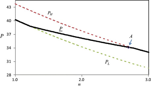
Moreover, it is dangerous for monetary authorities to target price level as policy instruments (Gaspar et al., 2010; Kahn, 2009). For example, at point $A$ in Figure 4, if central bank intends to lower price it might undertake contractionary monetary policies. However, the price remains the same even after such contractionary policies have taken effect because prices are identical in the high and low-demand states. Therefore, policymakers would further increase the magnitude of monetary policy. This action might then be too strong and could harm the manufacturers in highly competitive markets.

With the case of economies of scale ($f_1<0$), Figure 5 reveals a positive relation between market competition and price flexibility, which contrasts with that in Figure 4. Price is completely rigid when the market concentration is high ($n=1$), and starts to fluctuate in larger magnitude as the number of competitors increases. The economic intuition is that market competition increases supply across the market but decreases each incumbent player’s supply. As more competitors enter the game, the reduction of each player’s production leads to a higher unit cost given $f_1<0$; thus, based on Proposition 1 and Figure 2, a higher $f_1$ can enlarge price fluctuations. This result, that the industry with higher market concentration generates more rigid prices, is consistent with Means’ (1935) administered price hypothesis, which suggested that firms with a degree of market power would choose to lower output rather than prices during recessionary periods. Geroski (1992) found that pricing dynamics are more sluggish in less competitive industries in the U.K. Carlton (1986) and Caucutt et al. (1999) concluded that seller concentration has a statistically significant positive influence on rigidity in manufacturing industries in the U.S. The divergent effects of Figure 4 and Figure 5 in relation to conflicting empirical results present the importance of theoretical underpinnings.

Figure 5. Negative $f_1$, numbers of firm and price rigidity.

Parameter values: $a=50,b=1,X=1,v=0.035,r=0.02,f_0=2.5,f_1=-0.1,s=0$

4. Product differentiation

Sellers can insulate themselves from price competition through locations, atmosphere, and sales services. The higher the level of differentiation in product markets, the higher the levels of profitability seem to be (Davies, 2001). However, the association between seller differentiation and price flexibility is rarely discussed in the literature. This section specifies $n=2$ follows Section 3 in order to construct a model with differentiated manufacturers. At $T=1$, the demand functions faced by the two sellers respectively can be written as follows: (32) $$p_1=\frac{\mathit{aX}}{b}-\frac{(q_1+\theta q_2)}{b},$$(32) (33) $$p_2=\frac{\mathit{aX}}{b}-\frac{(\theta q_1+q_2)}{b},$$(33)

Where $\theta$ is the inverse of the degree of product differentiation or the degree of product homogeneity, ranging from 0 when players are independent of one another to 1 when players are perfect substitutes. Suppose that two manufacturers have a similar cost function, we have Lagrangian for the manufacturer $i$ as follow: (34) $$\begin{array}{c}{\mathcal{L}}_i=\left(-f_0-f_1{q}_i\right)q_i+m(\frac{a}{b}X{}_H-\frac{q_i+\theta q_j}{b})q_i+u{\underset{\_}{\mathit{p}}}_i(\mathit{aX}{}_L-\theta q_j-b{\underset{\_}{\mathit{p}}}_i)+\mathit{us}(q_i-(\mathit{aX}{}_L-q_j\theta -b{\underset{\_}{\mathit{p}}}_i))\\ +{\lambda }_1(\frac{\mathit{aX}{}_H}{b}-\frac{(q_i+\theta q_j)}{b}-{\underset{\_}{\mathit{p}}}_i)+{\lambda }_2({\underset{\_}{\mathit{p}}}_i-\frac{\mathit{aX}{}_L}{b}+\frac{(q_i+\theta q_j)}{b}),i,j=1,2.\end{array}$$(34)

Lemma 3: Suppose that demand functions faced by two differentiated manufacturers are Equation (32)–(33), respectively, where $\theta$ ranging from 0 when manufacturers are independent of one another to 1 when manufacturers are perfect substitutes. Two manufacturers have identical cost structures and engage in Cournot competition, their optimal production output $q_i$ and price floor ${\underset{\_}{\mathit{p}}}_i,i=1,2$, can be obtained as follows: (35) $$\begin{array}{c}{q}_i=\frac{\mathit{amX}{}_H+\mathit{bus}-b{f}_0}{2f_{1}b+2m+\theta m},{\underset{\_}{\mathit{p}}}_i=\frac{\mathit{aX}{}_L}{2b}+\frac{s}{2}-\frac{\theta q}{2b}\\ \text{If}\frac{2ab{f}_1{X}_L+\mathit{am}(2+\theta )(X_L-X_L)+b(2+\theta )f_0}{b(2f_{1}b+(2+\theta )e^{-\mathit{rt}})}<s<\frac{4ab{X}_H{f}_1-2f_{1}ab{X}_L+\mathit{am}(2+\theta )(X_H-X_L)+b(2+\theta )f_0}{b(2f_{1}b+(2+\theta )e^{-\mathit{rt}})},\end{array}$$(35) (36) $$q_i=\frac{a{X}_H{e}^{-\mathit{rt}}+\mathit{au}(X_H-X_L)-b{f}_0}{2f_{1}b+(2+\theta )e^{-\mathit{rt}}}\text{if}\frac{4ab{X}_H{f}_1-2f_{1}ab{X}_L+\mathit{am}(2+\theta )(X_H-X_L)+b(2+\theta )f_0}{b(2f_{1}b+(2+\theta )e^{-\mathit{rt}})}\le s<\frac{a{X}_L}{b},$$(36) (37) $$q_i=\frac{\mathit{am}{X}_H+\mathit{au}{X}_L-b{f}_0}{2f_{1}b+(2+\theta )e^{-\mathit{rt}}} \text{if} s\le \frac{2ab{f}_1{X}_L+\mathit{am}(2+\theta )(X_L-X_L)+b(2+\theta )f_0}{b(2f_{1}b+(2+\theta )e^{-\mathit{rt}})}.$$(37)

Proof:

Please see Appendix.

When competing products become more homogeneous, price competition in the market intensifies even the number of competitors remain the same. Proposition 3 shows that the relation between product homogeneity and price rigidity are not unidirectional but depends on the economics of scale.

Proposition 3:

The price rigidity is positively related to the product homogeneity $\theta$ as unit cost is an increasing function of output. The reverse is true when the unit cost is a decreasing function of output.

Proof:

Please see Appendix.

Proposition 3 explains why we cannot obtain consistent empirical results for the relation between product homogeneity and price rigidity until the cost factors have been taken into consideration. The markets filled with homogeneous competitors could exhibit price inertia given industry characterised by businesses with decreasing returns of scale, such as independent restaurants and other labor-intensive firms. However, the markets filled with homogeneous competitors also can produce obvious price fluctuations given industry characterised by economies of scale, such as panel and steel. The intuition behind conflicting results is a positive relation between average costs and price flexibility. In the industries with economies of scale, the production for each firm shrinks as players become more homogeneous, a hike of average cost adds pressure on inventory liquidation during economic recessions, thus leads to price fluctuations as stated in Proposition 1.

5. Conclusion

Economists traditionally regard the monopoly power as the cause behind price rigidity. The absence of economic underpinning on price rigidity could bring undesirable results in practices, such as monetary policies, antitrust policies, and marketing strategies. When market power is inaccurately regarded as the reason behind price rigidity, monetary policies can be too drastic for small businesses. If price inertia is misled as an evidence of monopoly, the antitrust investigation into price manipulations might end up suppressing competition. Further, in the field of marketing, inaccurate interpretation of the association among costs, output, and price adjustments could persuade marketing managers to devise inappropriate price promotions.

In light of theory vacancy, this study assumes that a risk-neutral manufacturer selects output and price floor before the realisation of stochastic demand, and defines the degree of price flexibility as the distance between price floor and high-demand-state price. The manufacturers set a price floor in order to preserve revenue in low-demand state conditional on positive salvage value of the unsold merchandise. This study shows that the salvage value and unit cost have divergent effects on the extent of price adjustments. While a positive salvage value relieves the pressure of inventory liquidation during the sluggish demand, the unit cost does the opposite. Our model also points out the ties between price rigidity and market competition but the directions could be divergent on distinctive cost structures. While the industry is characterised by decreasing returns to scale (unit cost is an increasing function of output), market competition is positively related to price rigidity. The reverse is true when the industry is characterised by economies of scale (unit cost is a decreasing function of output). The effect of product homogeneity on price rigidity resembles those of market competition, suggesting empirical research will not produce conclusive results until cost structures being considered in the future studies.

Appendix

Proof of Lemma 1.

Proof: If $\frac{a{X}_H}{b}-\frac{Q}{b}>\underset{\_}{\mathit{P}}>\frac{a{X}_L}{b}-\frac{Q}{b}$, the Kuhn–Tucker conditions $\frac{\partial L}{\partial {\lambda }_1},\frac{\partial L}{\partial {\lambda }_2}>0$ are naturally satisfied. Since the two constraints are not binding, one can assume ${\lambda }_1={\lambda }_2=0$, and the first-order conditions become: (11) $$\frac{\partial \mathcal{L}}{\partial Q}=-f_0-2f_{1}Q+m(\frac{a{X}_H}{b}-\frac{2Q}{b})+\mathit{us}=0,$$(11) (12) $$\frac{\partial \mathcal{L}}{\partial \underset{\_}{\mathit{P}}}=\mathit{au}{X}_u-2bu\underset{\_}{\mathit{P}}+\mathit{ubs}=0.$$(12)

Solving for $Q$ and $\underset{\_}{\mathit{P}}$ yields: (8) $$Q=\frac{\mathit{am}{X}_H+\mathit{bus}-b{f}_0}{2f_{1}b+2m},\begin{array}{c}\end{array}\underset{\_}{\mathit{P}}=\frac{a{X}_L}{2b}+\frac{s}{2}.$$(8)

The following second-order sufficient conditions for maximum profit are automatically satisfied given Assumption 2: $$\frac{\partial \mathcal{L}}{\partial Q}=-2f_1-\frac{2m}{b}<0,\begin{array}{c}\end{array}\frac{\partial \mathcal{L}}{\partial \underset{\_}{\mathit{P}}}=-2bu<0,\begin{array}{c}\end{array}\frac{\partial \mathcal{L}}{\partial Q}\frac{\partial \mathcal{L}}{\partial \underset{\_}{\mathit{P}}}-\frac{{\partial }^2\mathcal{L}}{\partial Q\partial \underset{\_}{\mathit{P}}}=4(f_1+\frac{m}{b})(\mathit{bu})-0>0.$$

Substituting equilibrium price floor and quantity into $\frac{a{X}_H}{b}-\frac{Q}{b}>\underset{\_}{\mathit{P}}>\frac{a{X}_L}{b}-\frac{Q}{b}$ produces the range of salvage value. If $\underset{\_}{\mathit{P}}=\frac{a{X}_H}{b}-\frac{Q}{b}$, the constraint $\underset{\_}{\mathit{P}}=\frac{a{X}_L}{b}-\frac{Q}{b}$ cannot be binding, and thus we assume that ${\lambda }_2=0$. The first-order conditions therefore become $\frac{\partial \mathcal{L}}{\partial Q}=\frac{\partial \mathcal{L}}{\partial \underset{\_}{\mathit{P}}}=\frac{\partial \mathcal{L}}{\partial {\lambda }_1}=0$. (13) $$\left[\begin{array}{ccc}-2f_1-\frac{2m}{b}& 0& \frac{1}{b}\\ 0& -2bu& 1\\ \frac{1}{b}& 1& 0\end{array}\right]\left[\begin{array}{c}Q\\ \underset{\_}{\mathit{P}}\\ {\lambda }_1\end{array}\right]=\left[\begin{array}{c}\\ \end{array}\begin{array}{c}{f}_0-\frac{\mathit{am}{X}_H}{b}-\mathit{us}\\ -\mathit{au}{X}_L-\mathit{usb}\\ \frac{a}{b}{X}_H\end{array}\right].$$(13)

Solving these equations yields Equation (9). The second-order sufficient condition requires that the following boarded Hessian be positive: (14) $$\left|\begin{array}{ccc}-2f_1-2m/b& 0& 1/b\\ 0& -2bu& 1\\ 1/b& 1& 0\end{array}\right|=2(f_1+m/b)+2u.$$(14)

This is satisfied if $f_1>-m{b}^{-1}$, which is given by Inequality (6(6) $$f_1>-\frac{\alpha e^{-\mathit{rt}}}{b}.$$(6) ) in Assumption 2. Following the same procedure, one can obtain Equation (10)(10) $$\begin{array}{c}Q=\frac{\mathit{am}{X}_H+\mathit{au}{X}_L-b{f}_0}{2f_{1}b+2e^{-\mathit{rt}}}\\ \text{if}\underset{\_}{\mathit{P}}=\frac{a{X}_L}{b}-\frac{Q}{b}\text{or}s\le \frac{4\mathit{ab}{f}_1{X}_L-2am{X}_H+4\mathit{am}{X}_L+2b{f}_0}{b(2f_{1}b+2m+2u)}.\end{array}$$(10) under the constraint $\underset{\_}{\mathit{P}}=\frac{a{X}_L}{b}-\frac{Q}{b}$.

Q.E.D.

Proof of Proposition 1.

Proof: When $\frac{4\mathit{ab}{f}_1{X}_L-2am{X}_H+4\mathit{am}{X}_L+2b{f}_0}{b(2f_{1}b+2m+2u)}<s<\frac{4ab{X}_H{f}_1-2f_{1}ab{X}_L+2am(X_H-X_L)+2b{f}_0}{b(2f_{1}b+2m+2u)}$ or $\frac{a{X}_H}{b}-\frac{Q}{b}>\underset{\_}{\mathit{P}}>\frac{a{X}_L}{b}-\frac{Q}{b}$, we define the difference between the high-demand price and price floor as: (15) $$D=(\frac{a{X}_H}{b}-\frac{\mathit{am}{X}_H+\mathit{bus}-b{f}_0}{2f_1{b}^2+2mb})-(\frac{a{X}_L}{2b}+\frac{s}{2}).$$(15)

A higher $D$ represents a higher degree of price flexibility. Hence, differentiating Equation (15)(15) $$D=(\frac{a{X}_H}{b}-\frac{\mathit{am}{X}_H+\mathit{bus}-b{f}_0}{2f_1{b}^2+2mb})-(\frac{a{X}_L}{2b}+\frac{s}{2}).$$(15) with respect to $s$ yields: (16) $$\frac{\mathit{dD}}{\mathit{ds}}=-\frac{u}{2f_{1}b+2m}-\frac{1}{2}<0.$$(16)

Equation (16)(16) $$\frac{\mathit{dD}}{\mathit{ds}}=-\frac{u}{2f_{1}b+2m}-\frac{1}{2}<0.$$(16) indicates that a higher salvage value narrows the magnitude of price fluctuations. Differentiating Equation (15)(15) $$D=(\frac{a{X}_H}{b}-\frac{\mathit{am}{X}_H+\mathit{bus}-b{f}_0}{2f_1{b}^2+2mb})-(\frac{a{X}_L}{2b}+\frac{s}{2}).$$(15) with respect to $f_0$ and $f_1$ yields: (17) $$\frac{\mathit{dD}}{d{f}_0}=\frac{1}{2f_{1}b+2m}>0,$$(17) (18) $$\frac{\mathit{dD}}{d{f}_1}=\frac{2(\mathit{am}{X}_H+\mathit{bus}-b{f}_0)}{{(2f_{1}b+2m)}^2}>0.$$(18)

Equations (17)(17) $$\frac{\mathit{dD}}{d{f}_0}=\frac{1}{2f_{1}b+2m}>0,$$(17) and (18)(18) $$\frac{\mathit{dD}}{d{f}_1}=\frac{2(\mathit{am}{X}_H+\mathit{bus}-b{f}_0)}{{(2f_{1}b+2m)}^2}>0.$$(18) prove that a higher cost expands the price fluctuations under the given demand uncertainty. (19) $$\frac{\mathit{dD}}{\mathit{dt}}=\frac{-(a\frac{\mathit{dm}}{\mathit{dt}}{X}_H+b\frac{\mathit{du}}{\mathit{dt}}s+b{f}_0)(2f_1{b}^2+2mb)-(\mathit{am}{X}_H+\mathit{bus}-b{f}_0)\cdot 2\frac{\mathit{dm}}{\mathit{dt}}b}{{(2f_1{b}^2+2mb)}^2}.$$(19)

Because $\mathit{dm}/\mathit{dt}=-r\alpha e^{-\mathit{rt}}<0$, one can ensure $\mathit{dD}/\mathit{dt}>0$.

Q.E.D.

Proof of Lemma 2.

Proof: When $\frac{a{X}_H}{b}-\frac{Q}{b}>{\underset{\_}{\mathit{p}}}_i>\frac{a{X}_L}{b}-\frac{Q}{b}$, letting ${\lambda }_1={\lambda }_2=0$ and differentiating Equation (21)(21) $$\begin{array}{c}\mathcal{L}=\left(-f_0-f_{1}q{}_i\right)q_i+m(\frac{a}{b}{X}_H-\frac{Q}{b})q_i+u{\underset{¯}{\mathit{P}}}_i(a{X}_L-Q_{-i}-b{\underset{¯}{\mathit{p}}}_i)+\mathit{us}(Q-(a{X}_L-Q_{-i}-b{\underset{¯}{\mathit{p}}}_i))\\ \begin{array}{c}\end{array}+{\lambda }_1(\frac{a{X}_H}{b}-\frac{Q}{b}-{\underset{¯}{\mathit{p}}}_i)+{\lambda }_2({\underset{¯}{\mathit{p}}}_i-\frac{a{X}_L}{b}+\frac{Q}{b}).\end{array}$$(21) with respect to $q_i$ and ${\underset{\_}{\mathit{p}}}_i$ yields: (25) $$(2f_1+\frac{2m}{b})q_i+\frac{m}{b}{Q}_{-i}=\frac{\mathit{am}}{b}{X}_H-f_0+\mathit{us},$$(25) (26) $${\underset{\_}{\mathit{p}}}_i=\frac{a}{2b}{X}_L+\frac{s}{2}-\frac{Q_{-i}}{2b}.$$(26)

Differentiating Equation (21)(21) $$\begin{array}{c}\mathcal{L}=\left(-f_0-f_{1}q{}_i\right)q_i+m(\frac{a}{b}{X}_H-\frac{Q}{b})q_i+u{\underset{¯}{\mathit{P}}}_i(a{X}_L-Q_{-i}-b{\underset{¯}{\mathit{p}}}_i)+\mathit{us}(Q-(a{X}_L-Q_{-i}-b{\underset{¯}{\mathit{p}}}_i))\\ \begin{array}{c}\end{array}+{\lambda }_1(\frac{a{X}_H}{b}-\frac{Q}{b}-{\underset{¯}{\mathit{p}}}_i)+{\lambda }_2({\underset{¯}{\mathit{p}}}_i-\frac{a{X}_L}{b}+\frac{Q}{b}).\end{array}$$(21) with respect to $q_i,i=2..n$ gives $n-1$ equations, with Equation (25)(25) $$(2f_1+\frac{2m}{b})q_i+\frac{m}{b}{Q}_{-i}=\frac{\mathit{am}}{b}{X}_H-f_0+\mathit{us},$$(25) we have $n$ equation describe the relationship among $q_i,i=1..n$. With $n$ equations, one can solve output for $n$ firms; the results show that each firm’s output is the same, so we have $q_i=\frac{\mathit{am}{X}_H+\mathit{bus}-b{f}_0}{2f_{1}b+(n+1)m},i=1..n$. Differentiating Equation (21)(21) $$\begin{array}{c}\mathcal{L}=\left(-f_0-f_{1}q{}_i\right)q_i+m(\frac{a}{b}{X}_H-\frac{Q}{b})q_i+u{\underset{¯}{\mathit{P}}}_i(a{X}_L-Q_{-i}-b{\underset{¯}{\mathit{p}}}_i)+\mathit{us}(Q-(a{X}_L-Q_{-i}-b{\underset{¯}{\mathit{p}}}_i))\\ \begin{array}{c}\end{array}+{\lambda }_1(\frac{a{X}_H}{b}-\frac{Q}{b}-{\underset{¯}{\mathit{p}}}_i)+{\lambda }_2({\underset{¯}{\mathit{p}}}_i-\frac{a{X}_L}{b}+\frac{Q}{b}).\end{array}$$(21) with respect to ${\underset{\_}{\mathit{p}}}_i,i=2..n$ gives $n-1$ equations, with Equation (26)(26) $${\underset{\_}{\mathit{p}}}_i=\frac{a}{2b}{X}_L+\frac{s}{2}-\frac{Q_{-i}}{2b}.$$(26) we have $n$ equation describing the relationship between each firm’s price floor and other players’ output. Substituting $q_i=\frac{\mathit{am}{X}_H+\mathit{bus}-b{f}_0}{2f_{1}b+(n+1)m},i=2..n$ into Equation (26)(26) $${\underset{\_}{\mathit{p}}}_i=\frac{a}{2b}{X}_L+\frac{s}{2}-\frac{Q_{-i}}{2b}.$$(26) , one can solve price floor for $p_1$, iterating the same procedure we can have ${\underset{\_}{\mathit{p}}}_2,{\underset{\_}{\mathit{p}}}_3\dots {\underset{\_}{\mathit{p}}}_n$. Substituting equilibrium $q_i$ and ${\underset{\_}{\mathit{p}}}_i$ into $\frac{a{X}_H}{b}-\frac{Q}{b}>{\underset{\_}{\mathit{p}}}_i>\frac{a{X}_L}{b}-\frac{Q}{b}$ gives a condition $\frac{2\mathit{ab}{f}_1{X}_L+\mathit{am}(n+1)(X_L-X_L)+b(n+1)f_0}{b(2f_{1}b+(+(n+1)m+(n+1)u)}<s<\frac{4ab{X}_H{f}_1-2f_{1}ab{X}_L+\mathit{am}(n+1)(X_H-X_L)+b(n+1)f_0}{b(2f_{1}b+(+(n+1)m+(n+1)u)}$.

When ${\underset{\_}{\mathit{p}}}_i=\frac{a{X}_H}{b}-\frac{Q}{b}$, the solutions can be obtained by solving the following equations: (27) $$\left[\begin{array}{ccc}-2f_1-\frac{2m}{b}& 0& \frac{1}{b}\\ 0& -2bu& 1\\ \frac{1}{b}& 1& 0\end{array}\right]\left[\begin{array}{c}{q}_i\\ {\underset{\_}{\mathit{p}}}_i\\ {\lambda }_1\end{array}\right]=\left[\begin{array}{c}\\ \end{array}\begin{array}{c}{f}_0-\frac{\mathit{am}{X}_H}{b}-\mathit{us}+\frac{m{Q}_{-i}}{b}\\ -\mathit{au}{X}_L-\mathit{usb}+u{Q}_{-i}\\ \frac{a}{b}{X}_H+\frac{Q_{-i}}{b}\end{array}\right].$$(27)

Solving these equations yields Equation (23)(23) $$q_i=\frac{a{X}_H{e}^{-\mathit{rt}}+\mathit{au}(X_H-X_L)-b{f}_0}{2f_{1}b+(n+1)e^{-\mathit{rt}}}\text{if}\frac{4ab{X}_H{f}_1-2f_{1}ab{X}_L+\mathit{am}(n+1)(X_H-X_L)+b(n+1)f_0}{b(2f_{1}b+(+(n+1)m+(n+1)u)}\le s<\frac{a{X}_L}{b},$$(23) . Following the same procedure, one can obtain Equation (24)(24) $$q_i=\frac{\mathit{am}{X}_H+\mathit{au}{X}_L-b{f}_0}{2f_{1}b+(n+1)e^{-\mathit{rt}}}\text{if}s\le \frac{2\mathit{ab}{f}_1{X}_L+\mathit{am}(n+1)(X_L-X_L)+b(n+1)f_0}{b(2f_{1}b+(+(n+1)m+(n+1)u)}.$$(24) under the constraint ${\underset{\_}{\mathit{p}}}_i=\frac{a{X}_L}{b}-\frac{Q}{b}$. The second-order conditions are the same as those in Lemma 1, which requires that Inequality (6(6) $$f_1>-\frac{\alpha e^{-\mathit{rt}}}{b}.$$(6) ) holds ($f_1>-m{b}^{-1}$).

Q.E.D.

Proof of Proposition 2.

Proof: When $\frac{2\mathit{ab}{f}_1{X}_L+\mathit{am}(n+1)(X_L-X_L)+b(n+1)f_0}{b(2f_{1}b+(+(n+1)m+(n+1)u)}<s<\frac{4ab{X}_H{f}_1-2f_{1}ab{X}_L+\mathit{am}(n+1)(X_H-X_L)+b(n+1)f_0}{b(2f_{1}b+(+(n+1)m+(n+1)u)}$ or $\frac{a{X}_H}{b}-\frac{Q}{b}>{\underset{\_}{\mathit{p}}}_i>\frac{a{X}_L}{b}-\frac{Q}{b}$, the difference between the high-demand price and price floor is: (28) $$D=(\frac{a{X}_H}{b}-\frac{\mathit{nq}}{b})-(\frac{a{X}_L}{2b}-\frac{(n-1)q}{2b}+\frac{s}{2}).$$(28)

Differentiating $D$ with respect to $n$ yields: (29) $$\frac{\mathit{dD}}{\mathit{dn}}=\left[-\frac{\partial q}{\partial n}(n+1)-q\right]{(2b)}^{-1}.$$(29)

Differentiating $q$ in Equation (22)(22) $$\text{If}\frac{2\mathit{ab}{f}_1{X}_L+\mathit{am}(n+1)(X_L-X_L)+b(n+1)f_0}{b(2f_{1}b+(+(n+1)m+(n+1)u)}<s<\frac{4ab{X}_H{f}_1-2f_{1}ab{X}_L+\mathit{am}(n+1)(X_H-X_L)+b(n+1)f_0}{b(2f_{1}b+(+(n+1)m+(n+1)u)},$$(22) with respect to $n$ yields: (30) $$\frac{\partial q}{\partial n}=-q\frac{m}{2f_{1}b+(n+1)m}.$$(30)

Substituting Equation (30)(30) $$\frac{\partial q}{\partial n}=-q\frac{m}{2f_{1}b+(n+1)m}.$$(30) into Equation (29)(29) $$\frac{\mathit{dD}}{\mathit{dn}}=\left[-\frac{\partial q}{\partial n}(n+1)-q\right]{(2b)}^{-1}.$$(29) gives: (31) $$\frac{\mathit{dD}}{\mathit{dn}}=\frac{-q{f}_1}{(2f_{1}b+(n+1)m)}.$$(31)

The sign of $\mathit{dD}/\mathit{dn}$ depends on the sign of $f_1$.

Q.E.D.

Proof of Lemma 3.

Proof: When $\frac{a{X}_H}{b}-\frac{(q_1+\theta q_2)}{b}>{\underset{\_}{\mathit{p}}}_i>\frac{a{X}_L}{b}-\frac{(q_1+\theta q_2)}{b}$, letting ${\lambda }_1={\lambda }_2=0$ and differentiating Equation (34)(34) $$\begin{array}{c}{\mathcal{L}}_i=\left(-f_0-f_1{q}_i\right)q_i+m(\frac{a}{b}X{}_H-\frac{q_i+\theta q_j}{b})q_i+u{\underset{\_}{\mathit{p}}}_i(\mathit{aX}{}_L-\theta q_j-b{\underset{\_}{\mathit{p}}}_i)+\mathit{us}(q_i-(\mathit{aX}{}_L-q_j\theta -b{\underset{\_}{\mathit{p}}}_i))\\ +{\lambda }_1(\frac{\mathit{aX}{}_H}{b}-\frac{(q_i+\theta q_j)}{b}-{\underset{\_}{\mathit{p}}}_i)+{\lambda }_2({\underset{\_}{\mathit{p}}}_i-\frac{\mathit{aX}{}_L}{b}+\frac{(q_i+\theta q_j)}{b}),i,j=1,2.\end{array}$$(34) with respect to $q_i$ and ${\underset{\_}{\mathit{p}}}_i$ yields: (38) $$(2f_1+\frac{2m}{b})q_i+\frac{m}{b}{q}_j=\frac{\mathit{am}}{b}{X}_H-f_0+\mathit{us},$$(38) (39) $${\underset{\_}{\mathit{p}}}_i=\frac{a}{2b}{X}_L+\frac{s}{2}-\frac{\theta q_j}{2b}.$$(39)

Replacing $i$ with $j$ in Equation (34)(34) $$\begin{array}{c}{\mathcal{L}}_i=\left(-f_0-f_1{q}_i\right)q_i+m(\frac{a}{b}X{}_H-\frac{q_i+\theta q_j}{b})q_i+u{\underset{\_}{\mathit{p}}}_i(\mathit{aX}{}_L-\theta q_j-b{\underset{\_}{\mathit{p}}}_i)+\mathit{us}(q_i-(\mathit{aX}{}_L-q_j\theta -b{\underset{\_}{\mathit{p}}}_i))\\ +{\lambda }_1(\frac{\mathit{aX}{}_H}{b}-\frac{(q_i+\theta q_j)}{b}-{\underset{\_}{\mathit{p}}}_i)+{\lambda }_2({\underset{\_}{\mathit{p}}}_i-\frac{\mathit{aX}{}_L}{b}+\frac{(q_i+\theta q_j)}{b}),i,j=1,2.\end{array}$$(34) and differentiating it, produces four equations, results in Equation (35)(35) $$\begin{array}{c}{q}_i=\frac{\mathit{amX}{}_H+\mathit{bus}-b{f}_0}{2f_{1}b+2m+\theta m},{\underset{\_}{\mathit{p}}}_i=\frac{\mathit{aX}{}_L}{2b}+\frac{s}{2}-\frac{\theta q}{2b}\\ \text{If}\frac{2ab{f}_1{X}_L+\mathit{am}(2+\theta )(X_L-X_L)+b(2+\theta )f_0}{b(2f_{1}b+(2+\theta )e^{-\mathit{rt}})}<s<\frac{4ab{X}_H{f}_1-2f_{1}ab{X}_L+\mathit{am}(2+\theta )(X_H-X_L)+b(2+\theta )f_0}{b(2f_{1}b+(2+\theta )e^{-\mathit{rt}})},\end{array}$$(35) could be obtained by solving them. Substituting equilibrium output and price floor into $\frac{a{X}_H}{b}-\frac{(q_1+\theta q_2)}{b}>{\underset{\_}{\mathit{p}}}_i>\frac{a{X}_L}{b}-\frac{(q_1+\theta q_2)}{b}$ gives the condition of salvage value range. When $\underset{\_}{\mathit{P}}=\frac{a{X}_H}{b}-\frac{(q_i+\theta q_j)}{b}$, we derive Equation (35)(35) $$\begin{array}{c}{q}_i=\frac{\mathit{amX}{}_H+\mathit{bus}-b{f}_0}{2f_{1}b+2m+\theta m},{\underset{\_}{\mathit{p}}}_i=\frac{\mathit{aX}{}_L}{2b}+\frac{s}{2}-\frac{\theta q}{2b}\\ \text{If}\frac{2ab{f}_1{X}_L+\mathit{am}(2+\theta )(X_L-X_L)+b(2+\theta )f_0}{b(2f_{1}b+(2+\theta )e^{-\mathit{rt}})}<s<\frac{4ab{X}_H{f}_1-2f_{1}ab{X}_L+\mathit{am}(2+\theta )(X_H-X_L)+b(2+\theta )f_0}{b(2f_{1}b+(2+\theta )e^{-\mathit{rt}})},\end{array}$$(35) by solving the following bordered Hessian: $$\left[\begin{array}{ccc}-2f_1-\frac{2m}{b}& 0& \frac{1}{b}\\ 0& -2bu& 1\\ \frac{1}{b}& 1& 0\end{array}\right]\left[\begin{array}{c}{q}_i\\ {\underset{\_}{\mathit{p}}}_i\\ {\lambda }_1\end{array}\right]=\left[\begin{array}{c}\\ \end{array}\begin{array}{c}{f}_0-\frac{\mathit{am}{X}_H}{b}-\mathit{us}+\frac{m\theta q_j}{b}\\ -\mathit{au}{X}_L-\mathit{usb}+u\theta q_j\\ \frac{a}{b}{X}_H+\frac{\theta q_j}{b}\end{array}\right]$$

Replacing $a{X}_H/b$ in bordered Hessian with $a{X}_L/b$ produces Equation (37)(37) $$q_i=\frac{\mathit{am}{X}_H+\mathit{au}{X}_L-b{f}_0}{2f_{1}b+(2+\theta )e^{-\mathit{rt}}} \text{if} s\le \frac{2ab{f}_1{X}_L+\mathit{am}(2+\theta )(X_L-X_L)+b(2+\theta )f_0}{b(2f_{1}b+(2+\theta )e^{-\mathit{rt}})}.$$(37) . The second-order condition is satisfied given Assumption 2.

Q.E.D.

Proof of Proposition 3.

Proof: When $\frac{2\mathit{ab}{f}_1{X}_L+\mathit{am}(2+\theta )(X_L-X_L)+b(2+\theta )f_0}{b(2f_{1}b+(2+\theta )e^{-\mathit{rt}})}<s<\frac{4ab{X}_H{f}_1-2f_{1}ab{X}_L+\mathit{am}(2+\theta )(X_H-X_L)+b(2+\theta )f_0}{b(2f_{1}b+(2+\theta )e^{-\mathit{rt}})}$ or $\frac{a{X}_H}{b}-\frac{(1+\theta )q}{b}>{\underset{\_}{\mathit{p}}}_i>\frac{a{X}_L}{b}-\frac{(1+\theta )q}{b}$, the difference between the high-demand price and price floor is: (40) $$D=(\frac{a{X}_H}{b}-\frac{(1+\theta )q}{b})-(\frac{a{X}_L}{2b}-\frac{\theta q}{2b}+\frac{s}{2}).$$(40)

Differentiating $D$ with respect to $\theta$ yields: (41) $$\frac{\mathit{dD}}{d\theta }=\left[-\frac{\partial q}{\partial \theta }(\theta +2)-q\right]{(2b)}^{-1}.$$(41)

Based on Equation (35)(35) $$\begin{array}{c}{q}_i=\frac{\mathit{amX}{}_H+\mathit{bus}-b{f}_0}{2f_{1}b+2m+\theta m},{\underset{\_}{\mathit{p}}}_i=\frac{\mathit{aX}{}_L}{2b}+\frac{s}{2}-\frac{\theta q}{2b}\\ \text{If}\frac{2ab{f}_1{X}_L+\mathit{am}(2+\theta )(X_L-X_L)+b(2+\theta )f_0}{b(2f_{1}b+(2+\theta )e^{-\mathit{rt}})}<s<\frac{4ab{X}_H{f}_1-2f_{1}ab{X}_L+\mathit{am}(2+\theta )(X_H-X_L)+b(2+\theta )f_0}{b(2f_{1}b+(2+\theta )e^{-\mathit{rt}})},\end{array}$$(35) , the $\partial q/\partial \theta =-\mathit{qm}/(2f_1^{}b+2m+\theta m)$, substituting it into Equation (41)(41) $$\frac{\mathit{dD}}{d\theta }=\left[-\frac{\partial q}{\partial \theta }(\theta +2)-q\right]{(2b)}^{-1}.$$(41) one has: (42) $$\frac{\mathit{dD}}{d\theta }=\frac{-q{f}_1}{(2f_{1}b+(2+\theta )m)}.$$(42)

Assumption 2 assures that the denominator must be positive so the sign of Equation (42)(42) $$\frac{\mathit{dD}}{d\theta }=\frac{-q{f}_1}{(2f_{1}b+(2+\theta )m)}.$$(42) depends on $f_1$.

Q.E.D.

References

- Ball, Laurence, & Romer, David. (1991). Sticky Prices as Coordination Failure. American Economic Review, 81(3), 539–552.
- Bedrossian, A., & Moschos, D. (1988). Industrial structure, concentration and the speed of price adjustment. The Journal of Industrial Economics, 26, 459–475. doi: 10.2307/2098450
- Butz, David A. (1997). Vertical Price Controls with Uncertain Demand. Journal of Law and Economics, 40(2), 433–460.
- Carlton, D. W. (1986). The rigidity of prices. American Economic Review, 76, 637–658.
- Caucutt, E. M., Ghosh, M., & Kelton Christina, L. (1999). Durability versus concentration as an explanation for price inflexibility. Review of Industrial Organization, 14(1), 27–50. doi: 10.1023/A:1007723912369
- Chen, G. R. (2016). Dynamic model for market competition and price rigidity. Applied Economics, 48(36), 3485–3496. doi: 10.1080/00036846.2016.1139681
- Conlisk, J., Gerstner, E., & Sobel, J. (1984). Cyclic pricing by a durable goods monopolist. The Quarterly Journal of Economics, 99(3), 489–505. doi: 10.2307/1885961
- Cox, J. C., Ross, S. A., & Rubinstein, M. (1979). Option pricing: A simplified approach. Journal of Financial Economics, 7(3), 229–263. doi: 10.1016/0304-405X(79)90015-1
- Domberger, S. (1979). Price adjustment and market structure. The Economic Journal, 89(353), 96–108. doi: 10.2307/2231409
- Domberger, S. (1983). Industrial structure, pricing and inflation. Martin Robinson, UK: Oxford.
- Domowitz, I., Hubbard, R. G., & Petersen, B. C. (1986). Business cycles and the relationship between concentration and price-cost margins. The Rand Journal of Economics, 17(1), 1–17.
- Gaspar, V., Smets, F., & Vestin, D. (2010). Is the time for price-level path stability?. In P. Siklos, M. T. Bohl, & M. E. Wohar (Eds.), Challenges in central banking: The current institutional environment and forces affecting monetary policy. Cambridge: Cambridge University Press.
- Geroski, P. A. (1992). Price dynamics in UK manufacturing: A microeconomic view. Economica, 59(236), 403–419. doi: 10.2307/2554887
- Gordon, R. J. (1981). Output fluctuations and gradual price adjustment. Journal of Economic Literature, 19, 493–530.
- Greenslade, J. V., & Parker, M. (2012). New insights into price-setting behaviour in the UK: Introduction and survey results. The Economic Journal, 122(558), F1–15. doi: 10.1111/j.1468-0297.2011.02492.x
- Jullien, B., & Rey, P. (2007). Resale Price Maintenance and Collusion. The Rand Journal of Economics, 38(4), 983–1001. doi: 10.1111/j.0741-6261.2007.00122.x
- Kahn, G. A. (2009). Beyond inflation targeting: Should central banks target the price level? Federal Reserve Bank of Kansas City Economic Review, 2009, 35–64.
- Kraft, K. (1995). Determinants of price adjustment. Applied Economics, 27(6), 501–507. doi: 10.1080/00036849500000137
- Means, G. C. (1935). Industrial prices and their relative inflexibility. Paper Presented at the US Senate Document 13, 74th Congress, 1st Session, US Govt. Printing Office, Washington, DC.
- Meyer, J., & Cramon-Taubadel, S. (2004). Asymmetric price transmission: A survey. Journal of Agricultural Economics, 55(3), 581–611. doi: 10.1111/j.1477-9552.2004.tb00116.x
- Peltzman, S. (2000). Prices rise faster than they fall. Journal of Political Economy, 108(3), 466–502. doi: 10.1086/262126
- Powers, E. T., & Powers, N. J. (2001). The size and frequency of price changes: Evidence from grocery stores. Review of Industrial Organization, 18(4), 397–416.
- Schramm, R., & Sherman, R. (1977). A rationale for administered pricing. Southern Economic Journal, 44(1), 125–135. doi: 10.2307/1057306
- Serra, T., & Goodwin, B. K. (2003). Price transmission and asymmetric adjustment in the Spanish dairy sector. Applied Economics, 35(18), 1889–1899. doi: 10.1080/00036840310001628774
- Setiawan, M., Emvalomatis, G., & Oude, L. A. (2015). Price rigidity and industrial concentration: Evidence from the Indonesian food and beverages industry. Asian Economic Journal, 29(1), 61–72. doi: 10.1111/asej.12047
- Taylor, J. B. (2000). Low inflation, pass-through and the pricing power of firms. European Economic Review, 44(7), 1389–1408. doi: 10.1016/S0014-2921(00)00037-4
- Tirole, J. (1988). The theory of industrial organization. Cambridge, Mass: MIT Press.
- Weiss, C. R. (1995). Determinants of price flexibility in oligopolistic markets: Evidence from Austrian manufacturing firms. Journal of Economics and Business, 47(5), 423–439. doi: 10.1016/0148-6195(95)00036-4