Predicting the performance of equity anomalies in frontier emerging markets: a Markov switching model approach

Abstract

Equity anomalies in frontier markets appear and disappear over time. This article aims to demonstrate the predictability of which of these transient anomalies will be profitable using a Markov switching model. To do so, we examine 140 equity anomalies identified in the literature using a unique sample of over 3,600 stocks from 23 frontier equity markets between 1997 and 2016. The application of a Markov switching model reveals that the time-series pattern of expected returns is dependent upon the type of anomaly; some anomalies become unprofitable over time whereas profitability increases in tandem with the development of a specific stock market for other types of anomalies. Results further indicate that forecasts of the next month’s return obtained from this model can translate into profitable investment strategies. We find that an anomaly selection strategy that relies on the model produces abnormal returns and outperforms a naïve benchmark that considers all the anomalies. We go onto demonstrate that our results are robust.

Keywords:

• equity anomalies
• Markov switching model
• return predictability
• frontier equity markets
• emerging stock markets
• factor allocation

Jel codes:

• G12
• G14
• G15

1. Introduction

Equity anomalies are deceptive.¹ Although they are a popular topic in finance literature – potentially because they can translate into profits and bonuses for portfolio managers – they pose a challenge to researchers and investors. Although recent literature has identified hundreds of them (see, e.g., Green, Hand, & Zhang, 2017; Hou, Xue, & Zhang, 2017; Jacobs, 2015, 2016), they tend to disappear once discovered. Dimson and Marsh (1999) and McLean and Pontiff (2016) showed that as a result of investor learning and adaptation, many documented anomalies have ceased to exist.² It appears that when as a market develops and efficiency improves, the profitability of anomalies decreases.

However, recent studies by Cai et al. (2018) and Jacobs (2016) suggest the opposite. The authors argue that there are more equity anomalies in developed markets than in emerging ones. This suggests that as a market develops, anomalies tend to come to the fore rather than disappear. Regardless of the reality, a single conclusion is shared by all of these studies; expected returns on equity anomalies are not stable over time. Therefore, investors need a viable method of predicting the future performance of equity anomalies. The primary aim of this study is to offer such a method. In particular, the pertinent questions are as to whether an anomaly is still (or already) present and whether can investors profit from it.

In this study, we show that a Markov switching model may be used effectively to uncover the time-varying nature of expected returns and to predict the future performance of equity anomalies. We find that a portfolio of strategies with high predicted returns significantly outperforms a portfolio of anomalies with low predicted returns as well as a naïve benchmark that equal-weights anomaly portfolios.

To examine the time-varying nature of expected returns on anomalies, we conduct our investigations within frontier market equities. The analysis is performed using accounting and stock market data for more than 3,600 firms from 23 different countries in Africa, Asia, Europe and South America between 1997 and 2016. There are three reasons as to why we concentrate on frontier equities. Firstly, these markets offer a unique opportunity to observe the lifecycle of the development of market anomalies – from the inception of these markets. Secondly, they permit an out-of-sample examination of return patterns as frontier markets are largely an unexplored field in terms of equity anomalies. Thirdly, although the current size of frontier markets is relatively small, these markets have been growing rapidly in importance and prominence for global investors. For example, assets under management in dedicated active frontier market funds have increased from under US$1 billion in 2009 to more than US$9 billion in 2014 (Acadian, 2014).³

To investigate the behaviour of equity anomalies, we replicate and classify 140 strategies identified in the finance literature, based on the sample of Zaremba (2017b). Following Jacobs (2016), we use sorting procedures to form long-short portfolios. We also form meta-anomalies that aggregate multiple individual anomalies based on the basis similar underlying economic intuition. Subsequently, we apply a Markov switching model approach to uncover the time-series variation in expected returns on anomalies.

Finally, we evaluate whether the predictions of a Markov switching model can be translated into profitable strategies. To do so, we construct long-short portfolios of anomalies based upon forecasts obtained from a Markov switching model relating to the probability and expected returns of the following month’s regime. We then evaluate the performance of this portfolios using the Fama and French (1995) five-factor (F.F.5.F.) model.

This article proposes to contribute in two ways. First and foremost, we use a Markov switching model to uncover the time-varying expected returns on equity anomalies. Therefore, we reconcile the earlier seemingly conflicting results on disappearing and emerging anomalies (see Dimson & Marsh, 1999; Jacobs, 2016; McLean & Pontiff, 2016). We show that time-series patterns in expected returns depend strongly upon the type of anomaly.

Second, we demonstrate that the forecasts obtained using a Markov switching model may be successfully employed to predict performance and for the purposes of selecting the most promising equity anomaly strategies. Therefore, we offer a new anomaly-allocation instrument and expand upon the existing understanding of anomaly momentum (Avramov, Cheng, Schreiber, & Shemer, 2017; Ehsani, 2017; Zaremba & Szyszka, 2016), anomaly reversals (Arnott, Beck, & Kalesnik, 2016) and cross-sectional seasonalities in anomaly returns (Keloharju, Linnainmaa, & Nyberg, 2016; Zaremba, 2017a).

The findings of this study can be summarised as follows. First, out of the 140 equal-weighted (value-weighted) anomaly portfolios analysed, 56 (28) exhibit have C.A.P.M. alphas. By applying a Markov switching model to anomalies, we uncover time-series variation (changes over time) in expected returns on anomaly portfolios. For some categories, such as value investing, profitability has declined over time. Other strategies with initially insignificant gains, such as those based upon dividends or profitability, begin to yield significant payoffs in later stages of market development. Finally, there are also strategies with ambiguous time-varying patterns in expected returns that do not exhibit a distinct switch (change) over time.

Second, we demonstrate that forecasts provided by a Markov switching model can translate into profitable investment strategies. The anomalies that are identified as leading to positive and significant expected returns exhibit substantially higher subsequent payoffs than the anomalies that deliver negative or positive and insignificant expected returns. The results indicate that a long-short portfolio of anomalies that is long (short) in anomalies that are predicted to be profitable (unprofitable) on the basis of a Markov switching model yield a five-factor model alpha that exceeds 0.4% on a monthly basis and outperforms a naïve benchmark that equal weights all anomalies. The outcomes are robust to many considerations.

The remainder of the manuscript is organised as follows. Section 2 presents the data sources and the methodology used in constructing the sample. Section 3 outlines and discusses the performance of equity anomalies in frontier markets. Section 4 applies a Markov switching model to investigate the time-varying nature of expected returns on anomalies. Section 5 presents the results of the performance of anomaly-picking strategies that are based upon forecasts obtained using a Markov switching model. The last section concludes the article.

2. Data sources and sample construction

The sample used in this study comprises 23 stock markets classified as frontier markets by MSCI and that are included in the MSCI Frontier Markets Index. These are Argentina, Bahrain, Bangladesh, Bulgaria, Croatia, Estonia, Jordan, Kazakhstan, Kenya, Kuwait, Lebanon, Lithuania, Mauritius, Morocco, Nigeria, Oman, Pakistan, Romania, Serbia, Slovenia, Sri Lanka, Tunisia and Vietnam (MSCI, 2016).

We source our data from Bloomberg and include both listed and delisted firms to mitigate survivorship bias. Data manipulation is done using a monthly time series sample period of returns that spans the period between March 1998 and September 2016. Thus, the sample period includes a total of 223 monthly observations. We also utilise older data when necessary to estimate certain anomalies.

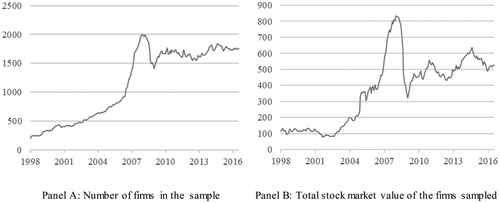
A firm is included in the sample if its return in month t and its total capitalisation at the end of month t-1 are both available. To ensure the quality of the sample and to align with market practice, we implement a few static and dynamic filters. As the sample comprises of only common stocks, we exclude closed-end funds, E.T.F.s, G.D.R.s and similar investment assets. We include equities for which the selected frontier countries are the primary markets. We also account for practical problems with so-called penny stocks and eliminate any firm from the sample in month t if at the end of month t-1 its nominal share price has dropped below US$0.20 or the total stock market capitalisation is below US$10 million. We also exclude observations with monthly returns of more than 500% or less than -98% as these most likely from the result of erroneously estimated stock split ratios (10 observations in total). Our final sample comprises of 3,621 firms and 255,079 monthly observations. The composition and evolution of the sample are presented in Table 1 and Figure 1, respectively.

Table 1. Geographical coverage of the research sample.

Country	Number of firms	Number of monthly observations	Country	Number of firms	Number of monthly observations
Argentina	98	11,977	Morocco	91	12,048
Bahrain	48	5146	Mauritius	83	7882
Bangladesh	260	10,912	Nigeria	54	2989
Bulgaria	156	8709	Oman	120	14,127
Croatia	235	16,227	Pakistan	305	23,736
Estonia	29	2699	Romania	272	9549
Jordan	226	21,719	Serbia	258	11,337
Kazakhstan	32	1152	Slovenia	99	7516
Kenya	54	5742	Sri Lanka	205	12,824
Kuwait	221	24,754	Tunisia	84	8647
Lebanon	11	1481	Vietnam	623	28,862
Lithuania	57	5044	Total	3621	255,079

Note: This table provides an overview of the geographical distribution of the sample. The number of monthly observations refers to periods for which both return and capitalisation data was available.

Figure 1. The research sample. Note. The figure presents the changes in the research sample over time.

All data has been converted into US dollars (US$) and we use the one-month U.S. T-bill rate from the Kenneth R. French data library as a proxy for the risk-free rate. ⁴

3. Equity anomalies in frontier markets

We examine 140 distinct cross-sectional patterns. The selection of anomalies closely follows from Zaremba (2017b) and is motivated by previous research on patterns in cross-sectional returns and includes the patterns investigated by Green et al. (2017), Hou et al. (2017) and Jacobs (2015, 2016).⁵ To be included in our sample, an anomaly must be identifiable from market and accounting data that is available in standard databases. As we require return data with a monthly frequency, the data must permit the derivation of returns on a monthly basis. A detailed description of the anomalies, their implementation and literature references are exhibited in Table A1 of supplementary material. We classified the anomalies into 20 categories based upon the underlying economic intuition and the correlation structure of their payoffs. This classification structure follows Zaremba (2017b).

On the basis of the 140 anomalies, we form portfolios by following a uniform procedure across all strategies. All stocks within the sample are sorted on anomaly-relevant variables as at the end of month t-1.⁶ Next, all stocks from the top and bottom 30% of the rankings are used to form equal-weighted and value-weighted portfolios. Finally, we construct zero-investment long-short portfolios. For each anomaly portfolio, we assume a long (short) position in the portfolio that should exhibit higher (lower) returns based upon the theoretical and empirical evidence. Thus, we expect all of the long-short strategies to exhibit positive returns.

In addition to individual anomalies, we also examine meta-anomalies as in Jacobs (2015). These are equal-weighted portfolios of all anomalies grouped according to the classification scheme set out in Table A1 in the supplementary material. We further aim to identify the underlying drivers of these anomalies – psychological, economic, institutional or anomalies specific. As evident from Table 3, this leads to the formation of 20 composite anomaly groups.

Table 2. Performance of equity meta-anomalies.

No.	Meta-anomaly	Panel A: Equal-weighted portfolios				Panel B: Value-weighted portfolios
		R		α		R		α
		Value	t-stat	Value	t-stat	Value	t-stat	Value	t-stat
1.	Value	0.93**	(6.66)	0.93**	(6.14)	0.48*	(2.55)	0.49*	(2.46)
2.	Dividends	0.19	(1.38)	0.19	(1.36)	0.33	(1.26)	0.33	(1.51)
3.	Profitability	0.37	(1.88)	0.36	(1.53)	0.47	(1.35)	0.46	(1.27)
4.	Credit risk and indebtedness	0.43**	(3.75)	0.43**	(3.07)	0.29	(1.66)	0.29	(1.15)
5.	Investment and intangibles	0.02	(0.32)	0.02	(0.10)	–0.14	(–0.34)	–0.14	(–0.49)
6.	Accruals	0.31	(1.86)	0.31	(1.26)	0.04	(0.12)	0.05	(0.13)
7.	Fundamental analysis	0.26*	(2.29)	0.26*	(2.31)	0.24	(1.88)	0.23	(1.66)
8.	Issuance	0.34*	(2.43)	0.34*	(2.45)	0.07	(0.32)	0.07	(0.33)
9.	Liquidity	0.29	(1.01)	0.28	(0.98)	–0.11	(–0.36)	–0.12	(–0.46)
10.	Low-volatility	0.63*	(2.19)	0.63	(1.95)	0.84*	(2.17)	0.83*	(1.98)
11.	Extreme and downside risk	–0.13	(–0.79)	–0.12	(–0.76)	–0.51*	(–2.03)	–0.49	(–1.58)
12.	Skewness	0.13	(1.00)	0.13	(1.00)	0.38	(1.69)	0.38	(1.55)
13.	Long-term reversal	0.41	(1.86)	0.41	(1.61)	0.31	(0.99)	0.31	(0.98)
14.	Short-term reversal	–1.17**	(–4.94)	–1.17**	(–4.78)	–0.94*	(–2.43)	–0.94**	(–2.58)
15.	Momentum	1.29**	(5.66)	1.28**	(5.34)	0.92**	(3.59)	0.91**	(2.90)
16.	Trend	1.15**	(3.88)	1.15**	(3.08)	0.42	(0.97)	0.42	(0.82)
17.	52-week high	1.31**	(5.55)	1.31**	(4.97)	1.07**	(3.88)	1.05**	(3.17)
18.	Seasonalities	0.72**	(4.14)	0.72**	(4.77)	0.49	(1.59)	0.49	(1.73)
19.	Analyst coverage	0.70**	(4.19)	0.70**	(2.75)	0.49*	(2.57)	0.49	(1.58)
20.	Market frictions and others	0.29**	(2.59)	0.29*	(2.47)	0.17	(0.79)	0.17	(0.81)

Note: This table reports the performance for meta-anomalies, i.e., portfolios that equally-weight all long-short anomaly portfolios from one-way sorts with a 30%-breakpoint according to the classifications in Table A1. No. is the number of anomalies considered. Meta-anomaly refers to groups of anomalies in Table 3. R is the mean monthly return, α is the intercept from the CAPM, and t-stat are corresponding t-statistics. The asterisks, * and **, indicate values that are significantly different from zero at the 5% and 1% levels of significance, The numbers in brackets are bootstrap (Newey and West [1987] robust standard error adjusted) t-statistics for the means (alphas).

Table 3. Performance of meta-anomalies under both regimes.

No.	Strategy group	Regime 1					Regime 2					LM
		µ		b		E(R)	µ		b		E(R)
		Value	t-stat	Value	t-stat		Value	t-stat	Value	t-stat
Panel A: Equal-Weighted Portfolios
1.	Value	0.97**	(4.71)	0.01	(0.15)	0.98**	0.44**	(2.90)	0.30*	(2.19)	0.63**	0.00
2.	Dividends	0.36**	(3.26)	0.21	(1.79)	0.45**	0.11	(0.65)	0.06	(0.72)	0.12	0.00
3.	Profitability	0.53**	(4.48)	0.23**	(2.83)	0.69**	–0.10	(–0.19)	0.07	(0.64)	–0.10	0.00
4.	Credit risk and indebtedness	0.31**	(3.51)	0.18*	(2.03)	0.38**	0.39	(1.14)	0.21	(1.80)	0.49	0.00
5.	Investment and intangibles	0.07	(0.16)	0.27*	(2.31)	0.10	–0.05	(–0.43)	0.03	(0.33)	–0.05	0.00
6.	Accruals	0.35	(0.90)	0.20*	(2.05)	0.43	0.08	(0.79)	0.28**	(3.19)	0.11	0.00
7.	Fundamental analysis	0.22**	(4.04)	0.02	(0.25)	0.23**	0.39	(1.10)	–0.12	(–0.98)	0.35	0.00
8.	Issuance	0.12	(0.70)	0.31	(1.33)	0.17	1.05	(0.61)	–0.69	(–1.14)	0.63	0.04
9.	Liquidity	0.29	(1.35)	0.16*	(2.34)	0.35	–0.24	(–0.08)	–0.03	(–0.11)	–0.23	0.00
10.	Low-volatility	0.30	(1.94)	0.27**	(3.64)	0.42	0.92	(1.24)	0.16	(1.38)	1.10	0.00
11.	Extreme and downside risk	0.05	(0.29)	0.25*	(2.13)	0.07	–0.18	(–0.70)	0.31**	(3.65)	–0.26	0.00
12.	Skewness	0.05	(0.68)	0.19**	(2.76)	0.07	0.52	(0.30)	0.06	(0.22)	0.56	0.00
13.	Long-term reversal	1.20	(1.94)	0.15	(1.27)	1.41	–0.04	(–0.22)	0.03	(0.36)	–0.04	0.00
14.	Short-term reversal	–1.02	(–1.93)	0.18	(1.62)	–1.25	–0.93**	(–3.33)	0.15	(1.31)	–1.09**	0.81
15.	Momentum	1.63**	(5.99)	–0.19	(–1.52)	1.37**	–0.33	(–0.38)	0.91**	(6.00)	–3.59	0.01
16.	Trend	1.22**	(2.94)	0.56**	(4.50)	2.81**	–0.02	(–0.03)	–0.28	(–1.24)	–0.02	5.21
17.	52-week high	1.55**	(6.00)	–0.09	(–0.82)	1.42**	0.25	(0.34)	0.80**	(3.95)	1.26	0.01
18.	Seasonalities	0.66**	(5.04)	0.10	(1.40)	0.73**	0.48	(0.33)	0.06	(0.22)	0.51	0.00
19.	Analyst coverage	0.42**	(4.46)	0.05	(0.52)	0.44**	0.89*	(2.07)	0.11	(1.15)	1.00*	0.00
20.	Market frictions and others	1.29**	(3.61)	–0.45**	(–3.17)	0.89**	0.00	(–0.01)	0.35**	(4.06)	0.00	0.00
Panel B: Value-Weighted Portfolios
1.	Value	1.01	(1.76)	0.04	(0.29)	1.05	0.18	(1.04)	–0.05	(–0.56)	0.17	0.00
2.	Dividends	0.79	(1.45)	0.01	(0.13)	0.80	0.05	(0.26)	–0.04	(–0.46)	0.05	0.00
3.	Profitability	0.46**	(2.80)	–0.12	(–1.38)	0.41**	0.53	(0.63)	0.07	(0.74)	0.57	0.00
4.	Credit risk and indebtedness	0.43	(0.95)	0.09	(0.90)	0.48	0.10	(0.81)	0.11	(1.23)	0.11	0.00
5.	Investment and intangibles	–0.17	(–0.22)	0.19	(1.56)	–0.21	–0.17	(–1.16)	0.11	(1.35)	–0.19	0.00
6.	Accruals	0.19	(0.32)	0.15	(1.60)	0.23	–0.31	(–1.92)	0.04	(0.45)	–0.32	0.00
7.	Fundamental analysis	0.14	(1.88)	–0.09	(–1.00)	0.12	0.39	(1.30)	–0.02	(–0.17)	0.38	0.00
8.	Issuance	0.01	(0.16)	0.26**	(2.86)	0.02	–0.03	(–0.05)	0.01	(0.16)	–0.03	0.00
9.	Liquidity	0.15	(0.72)	0.03	(0.26)	0.16	–0.59	(–0.89)	–0.12	(–1.07)	–0.53	0.00
10.	Low-volatility	0.58**	(2.90)	0.24	(1.93)	0.76**	0.95	(1.56)	0.09	(1.02)	1.04	0.00
11.	Extreme and downside risk	–0.19	(–0.94)	0.08	(1.03)	–0.21	–1.19	(–1.33)	0.17	(1.28)	–1.44	0.00
12.	Skewness	1.75*	(2.23)	–0.01	(–0.11)	1.73*	–0.10	(–0.99)	0.11	(1.33)	–0.11	0.00
13.	Long-term reversal	0.24	(0.48)	–0.33*	(–2.55)	0.18	0.23	(0.43)	0.70**	(4.83)	0.78	0.68
14.	Short-term reversal	–1.24	(–1.41)	0.10	(0.84)	–1.37	–0.61*	(–2.42)	–0.04	(–0.45)	–0.59*	0.00
15.	Momentum	1.05**	(4.48)	0.01	(0.07)	1.06**	0.40	(0.36)	0.27	(1.74)	0.55	0.00
16.	Trend	0.54	(1.51)	0.03	(0.31)	0.56	0.07	(0.07)	0.40**	(2.60)	0.11	0.00
17.	52-week high	1.17**	(5.53)	0.03	(0.33)	1.20**	0.66	(0.49)	0.30*	(1.99)	0.95	0.00
18.	Seasonalities	0.60**	(3.92)	–0.05	(–0.61)	0.57**	0.49	(0.69)	0.15	(1.33)	0.57	0.00
19.	Analyst coverage	0.41**	(2.81)	0.08	(0.87)	0.45**	0.47	(1.09)	0.14	(1.58)	0.55	0.00
20.	Market frictions and others	0.25	(1.14)	–0.26**	(–2.81)	0.19	0.06	(0.15)	0.89**	(5.60)	0.56	0.00

Note: This table reports the performance for the meta-anomalies, i.e., portfolios that equally weight the long-short anomaly portfolios according to the classification in Table A1 in the supplementary material, for two regimes as in Equation (4)(4) $$R_t={\mu }_{\left(s_i\right)}+b_{\left(s_i\right)}{R}_{t-1}+{\epsilon }_t\text{\hspace{0.5em}and\hspace{0.5em}}{\epsilon }_t\sim N(0,{\sigma }_{\left(s_i\right)}).$$(4) . No. is the number of anomalies considered. Meta-anomaly refers to groups of anomalies in Table 3, µ and b are parameters in Equation (3)(3) $$E\left(R_t\right)=\frac{\mu }{1-b},$$(3) and (4)(4) $$R_t={\mu }_{\left(s_i\right)}+b_{\left(s_i\right)}{R}_{t-1}+{\epsilon }_t\text{\hspace{0.5em}and\hspace{0.5em}}{\epsilon }_t\sim N(0,{\sigma }_{\left(s_i\right)}).$$(4) . L.M. is the p-value associated with the L.M. test statistic in Equation (10)(10) $$\mathit{LM}=2\mathrm{*}\left({\ell }_c\left(\mathit{\theta }\right)-\ell \left({\mathit{\theta }}_1\right)\right)$$(10) . The asterisks, * and **, indicate values that are significantly different from zero at the 5% and 1% levels of significance. The numbers in brackets are t-statistics.

To quickly scan the anomalies, in the first stages of analysis, we investigate the performance of the anomaly portfolios using the C.A.P.M. (Sharpe, 1964), which postulates that returns are solely determined by and related to movements in the market portfolio: (1) $$R_{i,t}={\alpha }_i+{\beta }_{\mathit{MKT},i}·\mathit{MKT}+{\epsilon }_{i,t},$$(1) where R_i,t, and MKT are excess returns on portfolio i and the market portfolio at time t, while α_i, and β_MKT,i are model parameters. The intercept, α_i, measures the average abnormal return (Jensen's alpha). The reason why we do not employ more sophisticated models at this stage is that our sample of anomalies includes return patterns – such as value, size, and momentum – that feature in a number popular asset pricing models.

Table A2 in the supplementary material reports the performance of the individual long-short anomaly portfolios. In total, only 62 (32) of the equal-weighted (value-weighted) strategies show positive and statistically significant mean returns (at the 5% level).⁷ Following adjustment for market risk, 56 (28) of the strategies result in statistically significant and positive abnormal returns. Although these results may initially appear unsatisfactory, they are consistent with earlier evidence that suggests that either due to data mining or improved market efficiency, the performance of numerous anomalies is questionable out-of-sample (see Dimson & Marsh, 1999; McLean & Pontiff, 2016). For example, Cai et al. (2018), who researched 16 popular anomalies in numerous countries around the world, report that only 20% (14%) of equal-weighted (value-weighted) anomalies yield significant payoffs in mainstream emerging markets.

Table 2 summarises the performance of meta-anomalies – portfolios that incorporate multiple individual anomaly strategies. The value effect (meta-anomaly 1) confirms its profitability, yield positive and abnormal returns across both equal-weighted and value-weighted portfolios. Analogously, the trend-related anomalies (meta-anomalies [15] – [16]) also exhibit cross-sectional predictive power. A reduction in the noise on individual ranking methodologies permits the emergence of additional patterns, undisclosed by the outcomes in Table A2 in the supplementary material. A number of further meta-strategies lead to positive and significant raw and abnormal returns for either equal-weighted or value-weighted portfolios. These include credit risk and indebtedness (meta-anomaly 4), fundamental analysis (meta-anomaly 7), issuance (meta-anomaly 8), low-volatility (meta-anomaly 10), seasonalities (meta-anomaly 18), analyst coverage (meta-anomaly 19) and the market friction and others (meta-anomaly 20) meta-anomaly strategies. Conversely, the short-term reversal phenomenon continues to produce losses. In summary, five meta-strategies are profitable for both equal-weighted and value-weighted portfolios and six anomalies result in significant payoffs for equal-weighted portfolios. However, the majority of the strategies are unprofitable.

4. Modelling the changing profitability of equity anomalies

As pointed out by Dimson and Marsh (1999), Cai et al. (2018), Jacobs (2016), and McLean and Pontiff (2016), the profitability of equity anomalies is not constant over time. Some anomaly strategies may become temporarily or structurally unstable while others may begin to yield abnormal returns as the market matures. To capture the time-varying nature of the equity anomalies, we apply a Markov switching model. We first outline its theoretical basis and then apply the model to meta-anomaly returns in frontier equity markets.

The aim of this exercise is to verify whether the anomaly returns could be characterised by two independent regimes. If so, then an investor may expect to use the Markov switching model as an effective tool for forecasting the anomaly performance.

Let ${\left(R_t\right)}_{t\in \mathbb{N}}$ denote returns on the meta-anomaly portfolios. To account for the presence of potential autocorrelation in monthly returns, the meta-anomalies may be modelled as an A.R.(1) process: (2) $$R_t=\mu +b{R}_{t-1}+{\epsilon }_t, {\epsilon }_t\sim N\left(0,\sigma \right).$$(2)

The optimal lag is selected using the standard information criteria and is found to be one. The expected value of an A.R.(1) process is given by: (3) $$E\left(R_t\right)=\frac{\mu }{1-b},$$(3)

Furthermore, if the process is stationary, then $\left|b<1\right|$.

As stated earlier, the aim of our approach is to account for the time-varying nature of expected returns on equity anomalies. Thus, to describe anomaly portfolio behaviour, we apply an A.R.(1) Markov switching model as follows: (4) $$R_t={\mu }_{\left(s_i\right)}+b_{\left(s_i\right)}{R}_{t-1}+{\epsilon }_t\text{\hspace{0.5em}and\hspace{0.5em}}{\epsilon }_t\sim N(0,{\sigma }_{\left(s_i\right)}).$$(4)

We allow coefficients associated with the expected value to switch between two different states, i.e., $s_t\in \left\{1,\mathrm{ }2\right\}$. The observation of either regime 1 or 2 at time t depends upon a realisation of an unobservable Markov chain. Thus, $s_t$ is conditioned on the following information set: $$R_{t-1}=\{s_{t-1}{,\mathrm{ }s}_{t-2},\dots .\}.$$

At any time where $\tau <t$, the regime that will prevail at time $t$ is unknown. Following Hamilton (1990), we introduce the following notation for conditional probabilities: (5) $${\widehat{\xi }}_{t|\tau }={\left[P\left(s_t=1|R_t;\mathit{\theta }\right),P\left(s_t=2|R_t\right)\right]}^T.$$(5)

We further assume that the transition probabilities from one regime to the other are defined as follows: $$P_t=\left[\begin{array}{cc}{p}_t^{11}& 1-p_t^{11}\\ 1-\mathrm{ }{p}_t^{22}& p_t^{22}\end{array}\right]$$ where $p_t^{\mathit{ij}}=P\left(s_t=j|s_{t-1}=i\right)$. Also, we assume that the transition matrix is constant. The estimation of unknown model parameters is performed using maximum likelihood estimation. Let $\mathit{\theta }$ denote all parameters of the unknown model and relevant log-likelihood function ${\ell }_c\left(\mathit{\theta }\right)\mathrm{ }$ has the following form: $${\ell }_c\left(\mathit{\theta }\right)=\sum _{t=1}^T\log \left(\sum _{j=1}^2{f}_j\left(r_t\right)P\left(s_t=j|{\mathcal{R}}_{t-1};\mathit{\theta }\right)\right),$$ where $f_j\left(r_t\right)$ is a density of returns in the $j$-regime (when $s_t=j$, j = 1, 2).

To find the maximum of ${\ell }_c\left(\mathit{\theta }\right)$, we apply the Hamilton filter (Hamilton, 1990). Let ${\eta }_t$ denote a vector of densities governed by $s_t$ at date $t$: (6) $${\eta }_t={\left[f_1\left(r_t\right),f_2\left(r_t\right)\right]}^T.$$(6)

The optimal inference and forecast for each month, $t$, in the sample can then be found by iteration using the following equations: (7) $${\widehat{\mathrm{ }\xi }}_{t|t}=\frac{{\widehat{\xi }}_{t|t-1}\odot \mathrm{ }{\eta }_t}{1^T\left({\widehat{\xi }}_{t|t-1}\odot \mathrm{ }{\eta }_t\right)},$$(7) (8) $${\widehat{\xi }}_{t+1|t}=P_t^T{\widehat{\xi }}_{t|t}.$$(8)

Where element by element multiplication is represented by ⊙. The log-likelihood function, ${\ell }_c\left(\mathit{\theta }\right)$, now has the following form: (9) $${\ell }_c\left(\mathit{\theta }\right)=\sum _{t=1}^T\log \left(1^T\left({\widehat{\xi }}_{t|t-1}\odot \mathrm{ }{\eta }_t\right)\right).$$(9)

The A.R.(1) model is nested within an A.R.(1) Markov switching model. If there is no statistically meaningful information in the two-regime model that predicts the profitability of an investment strategy, then a single regime model is followed. This can be established formally by testing the null hypothesis of an A.R.(1) model against an alternative of a two-regime model using the log-likelihood ratio test. The test statistic is then: (10) $$\mathit{LM}=2\mathrm{*}\left({\ell }_c\left(\mathit{\theta }\right)-\ell \left({\mathit{\theta }}_1\right)\right)$$(10) where ${\ell }_c\left(\mathit{\theta }\right)$) and $\ell \left({\mathit{\theta }}_1\right)$ are the likelihood functions of the unrestricted and restricted models. The test statistic follows a chi-square distribution with $\left(p-q\right)$ degrees of freedom where $p$ and $q$ is the number of unknown parameters in unrestricted and restricted models respectively.

On the basis of the A.R.(1) Markov switching model, we are able to obtain two regimes with different expected returns. The results in Table 3 provide insights into the time-varying nature of the meta-anomalies over two separate regimes. The last column of Table 3 reports the p-values associated with the L.M. test statistic for specification (10). Table 3 provides convincing evidence that for almost all of the anomalies the two regime Markov switching model provides a better description relative to a single-distribution alternative. This observation forms a solid foundation for the implementation of an anomaly selection strategy based on this method.

It appears that two individual distributions better approximate the universe of stock market anomalies and demonstrate the value of using two separate regimes to predict future returns. The results provide an overview of the characteristics of the two regimes. The left-hand-side columns of Panels A and B of Table 3 depict the regime with higher t-statistics associated with µ_(si). For a number of anomalies, the model indicates that there is only one profitable regime and the µ parameter is significant; in the other regime µ is statistically insignificant and indicative of a lack of profitability. Furthermore, while some anomalies remain significant under both regimes, their expected payoffs differ noticeably, and, also, a number of strategies are found to have an insignificant µ under both regimes. Nevertheless, for the majority of anomalies, the Markov switching model is a reliable method to approximate the return distribution and to predict future performance. This is in line with the findings of Dimson and Marsh (1999), Cai et al. (2016), Jacobs (2016), and McLean and Pontiff (2016) and others who report that the profitability and nature of equity anomalies are unstable over time. The results for the value-weighted portfolios are similar although the differences between regimes are less pronounced. However, almost all p-values are close to zero and this confirms the usefulness of the model in explaining and predicting returns on anomalies.

Figure 2 provides supplementary information that assists in gaining further insight into the results reported in Table 3. The individual figures (Panel A to L) indicate the probability at the end of month t that in month t-1 the anomaly will remain profitable – that is, remain under the first regime. For brevity, we only report the results for these anomalies for which at least one regime was associated with a significant µ. We also limit our discussion to the equal-weighted portfolios – the value-weighted strategies are reported in Figure A1 in the supplementary material.

Figure 2. Time series probabilities of remaining in a regime that results in significant positive returns. Note: This figure presents the probabilities of remaining in a regime that yields significant positive returns on meta-anomalies. Shaded areas represent the periods during which probability exceeds 0.5.

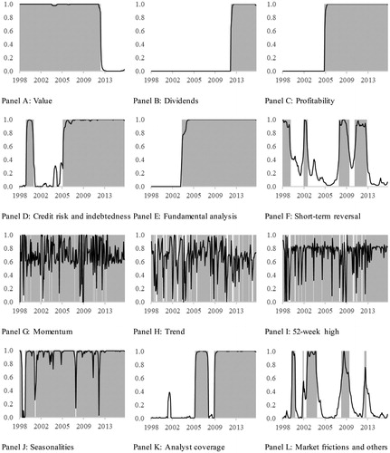
The meta-anomaly associated with the value effect (Panel A) exhibits behaviour that is in line with that observed by McLean and Pontiff (2016). This anomaly is found to be profitable and significant until 2012 after which it loses its ability to generate abnormal returns. In contrast, a number of meta-anomalies, for example, dividends (Panel B), profitability (Panel C), credit risk and indebtedness (Panel D), fundamental analysis (Panel E) and analyst coverage (Panel K), which are initially insignificant and unprofitable, subsequently transition to profitability. Some, such as fundamental analysis, transition at an earlier date (2003) whereas others, such as dividends, transition at later dates (2012). However, in all instances, the patter of transition is similar; profitability appears after a certain period of time. This supports the propositions of Jacobs (2016) that the more developed a stock market is, that the greater the number of anomalous patterns in cross-sectional returns.

Finally, there are anomalies for which the time-series variation is not as clear. Momentum (Panel G) and trend (Panel H) are two examples; these anomalies experience frequent switches between profitability and unprofitability which are potentially driven by external factors or an unknown process.

Summing, the application of the Markov switching model to the meta-anomaly portfolio confirms that the returns could be well described by two individual distributions, forming a promising starting point for the design of a relevant anomaly-picking strategy.

5. Asset allocation across anomalies

Having documented the time-series variation in expected returns on equity anomalies, we are interested in determining whether these patterns may be translated into profitable trading strategies. Therefore, we form portfolios of equal-weighted meta-anomalies which we predict will remain profitable (or unprofitable) and test their performance using an asset pricing model.

Our methodology for constructing anomaly portfolios is based upon the Markov switching model. The model requires a considerable amount of data estimate the regimes accurately and therefore we apply our model to the latest 53 monthly observations and use the first 170 monthly observations as a model training samples. For each month, months 171 to 223, we estimate our model using all observations available for these months. The training period is systematically extended to forecast to returns in the next month.

When forming the meta-anomaly portfolios, we consider two criteria that identify future regimes: (1) the forecasted probability of an observation to falling under a specific regime in the following month; and (2) the t-statistic associated with an estimated ${\mu }_{\left(s_i\right)}$ parameter for the following month’s most probable regime. In the first pass, we verify whether the probability of an observation of the most likely regime is sufficiently high – whether it exceeds a certain threshold of p. We use three different minimum levels for p: 0.5, 0.7, and 0.9 (corresponding to 50%, 70% and 90%, respectively). We then consider for inclusion in our portfolios the anomalies that are associated with forecasted probabilities that exceed the required thresholds. Subsequently, we determine whether the anomaly in the most likely next month’s regime is significantly profitable, i.e., whether the ${\mu }_{\left(s_i\right)}$ is positive and significantly different from zero at the 5% level of statistical significance. Following this test, we form two individual equal-weighted portfolios of meta-anomalies that include all anomalies that are predicted to be significantly profitable in the next month (i.e., ${\mu }_{\left(s_i\right)}$ is positive and statistically significant) and that is expected to not be positive and significantly profitable (i.e., ${\mu }_{\left(s_i\right)}$ is not simultaneously positive and significant). We classify these portfolios as profitable (Prof) and unprofitable (Unprof). To investigate differences in the performance of these two portfolios, we also form a long-short portfolio (P-U) which is long (short) in the Prof (Unprof) anomalies. Finally, we compare their performance with a benchmark portfolio that weights 20 meta-anomalies equally.

To evaluate the performance of the meta-anomaly portfolios, we apply the FF5F (2015) model: (10) $$R_t=\alpha +{\beta }_{\mathit{MKT}}{\mathit{MKT}}_t+{\beta }_{\mathit{SMB}}{\mathit{SMB}}_t+{\beta }_{\mathit{HML}}{\mathit{HML}}_t+{\beta }_{\mathit{RMW}}{\mathit{RMW}}_t+{\beta }_{\mathit{CMA}}{\mathit{CMA}}_t+{\epsilon }_t,$$(10) where ${\mathit{MKT}}_t$ is the excess market return (the market risk factor) observed at time t, SMB_t, HML_t, RMW_t, and CMA_t, are factor portfolios representing size, value, profitability and investment effects in the cross-section of returns and ${\beta }_{\mathit{MKT}}$, ${\beta }_{\mathit{SMB}}$, ${\beta }_{\mathit{HML}}$, ${\beta }_{\mathit{RMW}}$, ${\beta }_{\mathit{CMA}}$ are corresponding factor exposures. The intercept is denoted by $\alpha$ and ${\epsilon }_t$ is the random error term. Factor returns are calculated following the approach of Zaremba (2017b).

Table 4 reports the performance of profitable and unprofitable meta-anomalies selected using the Markov switching model. The results in the table show that the anomalies predicted as profitable outperform the unprofitable anomalies. The mean monthly returns on the Prof portfolios are always significantly positive, regardless of the required prediction probability and range between 0.46% and 0.55% (t-statistics between 4.94 and 7.10) The Unprof portfolios are characterised by mean monthly returns of between 0.04% and 0.13%, that are statistically indistinguishable from zero. The means returns on the long-short P-U portfolios are positive and statistically significant in all instances and range between 0.40% and 0.43% (t-statistics between 3.20 and 3.61). Furthermore, when the FF5F (2015) model is applied, the alphas on the long-short portfolios are statistically significant. Their magnitudes range between 0.41% and 0.45% (with the corresponding t-statistics between 2.67 and 3.20), depending upon the assumed probability forecast (50%, 70%, or 90%).

Table 4. Performance of portfolios of meta-anomalies formed using Markov switching model predictions.

	50% probability forecast			70% probability forecast			90% probability forecast			Benchmark portfolio
	Pro	Unprof	P-U	Prof	Unprof	P-U	Prof	Unprof	P-U
R	0.50**	0.10	0.40**	0.55**	0.13	0.43**	0.46**	0.04	0.42**	0.31**
	(4.94)	(1.74)	(3.20)	(6.12)	(1.81)	(3.61)	(7.10)	(0.48)	(3.66)	(5.61)
Vol	0.69	0.47	0.82	0.61	0.53	0.73	0.47	0.78	0.83	0.42
αFF5	0.46**	0.06	0.41**	0.53**	0.08	0.45**	0.47**	0.06	0.41**	0.28**
	(4.07)	(1.05)	(2.67)	(5.26)	(1.14)	(2.95)	(7.34)	(0.70)	(3.20)	(5.80)
MKT	–0.03	–0.01	–0.03	–0.02	–0.04	0.02	0.01	–0.08	0.10	–0.02
	(–0.85)	(–0.30)	(–0.52)	(–0.68)	(–1.29)	(0.40)	(0.47)	(–1.95)	(1.71)	(–0.90)
SMB	0.02	0.04	–0.02	0.00	0.00	0.00	–0.01	–0.03	0.02	0.03
	(0.40)	(1.30)	(–0.29)	(0.10)	(0.01)	(0.06)	(–0.30)	(–0.42)	(0.19)	(1.00)
HML	0.00	0.14**	–0.15	0.00	0.12*	–0.12	–0.05	0.10	–0.15	0.06
	(–0.03)	(3.36)	(–1.60)	(0.00)	(2.15)	(–1.69)	(–1.71)	(1.60)	(–1.90)	(1.80)
RMW	0.10*	0.08**	0.02	0.10**	0.11**	0.00	0.10**	0.13**	–0.03	0.09**
	(2.47)	(3.31)	(0.42)	(3.13)	(3.43)	(–0.04)	(3.93)	(3.34)	(–0.69)	(4.17)
CMA	0.04	0.08	–0.04	0.06	0.07	–0.01	0.07	0.14*	–0.08	0.07*
	(0.65)	(1.84)	(–0.39)	(1.08)	(1.54)	(–0.15)	(1.83)	(2.18)	(–0.90)	(2.54)
R^2	7.40	30.50	1.40	13.90	29.30	4.40	34.40	35.40	7.20	27.90

Note: This table reports the monthly returns on portfolios of equal-weighted meta-anomalies reported in Panel A in Table 2. Prof (Unprof) is an equal-weighted portfolio of meta-anomalies that is predicted to be in a regime with a positive significant (insignificant) µ parameter in Equation (4)(4) $$R_t={\mu }_{\left(s_i\right)}+b_{\left(s_i\right)}{R}_{t-1}+{\epsilon }_t\text{\hspace{0.5em}and\hspace{0.5em}}{\epsilon }_t\sim N(0,{\sigma }_{\left(s_i\right)}).$$(4) with a probability of profitability of at least 50% (Panel A), 70% (Panel B), or 90% (Panel C). The required significance level is 1%. P-U is a long-short portfolio which is long (short) in the Prof (Unprof) portfolios. The table also reports results for a benchmark portfolio that equal-weights all 20 meta-anomalies. R is the mean monthly return, Vol is the monthly standard deviation of returns, and α_FF5 is the intercept of the Fama and French (2015) five-factor model. The numbers in brackets (for R) are bootstrap (Newey and West (1987) robust standard error) adjusted (for α_FF5) t-statistics. Means, volatilities, and intercepts are expressed as percentages. The asterisks * and **, indicate values significantly different from zero at the 5% and 1% levels of significance.

Finally, strategies based upon predictions from the Markov switching model substantially outperform the equal-weighted benchmark comprising of all anomalies. The five-factor model alpha on the benchmark portfolio is 0.28% yet the Prof portfolios deliver monthly abnormal returns on that are between 66% and 91% higher.

In conclusion and with reference to the results in Table 4, the portfolios predicted to be profitable markedly outperform the meta-anomalies that are predicted to be unprofitable and the equal-weighted benchmark comprising all anomalies. As a robustness check, we relax some of the assumptions underlying our meta-anomaly picking strategies. Thus far, we have examined three different probability thresholds relating to next month’s regime, 50%, 70%, and 90%, and we also require that the anomalies are significantly profitable (${\mu }_{\left(s_i\right)}$). We now consider anomalies that are statistically at the 10% and 1% levels of significance extend our analysis of equal-weighted anomaly portfolios to value-weighted anomaly portfolios. Table 3 reports the five-factor model alphas on Prof, Unprof, and P-U portfolios for 15 new specifications that are the result of our robustness checks.

The results in Table 5 indicate that the efficiency of the anomaly-picking approach based upon the Markov switching model is robust to many considerations. The Prof portfolio displays higher five-factor alphas relative to the Unprof portfolios under different conditions. Outperformance is particularly strong for the equal-weighted anomaly portfolios (Panel A of Table 5); all long-short portfolios exhibit positive and significant abnormal returns between 0.37% and 0.48% per month. For the value-weighted portfolios, the alphas are generally lower and abnormal returns on differential portfolios are insignificant. Nevertheless, the signs on the alphas are always consistent (positive) and returns on weighted Prof portfolios are predominantly significant and higher than on the Unprof strategies. In conclusion, our results appear to be robust alternative specifications and methodologies.

Table 5. Monthly returns on alternative portfolios of meta-anomalies formed using Markov switching model predictions.

	50% probability forecast			70% probability forecast			90% probability forecast
	Prof	Unprof	P-U	Prof	Unprof	P-U	Prof	Unprof	P-U
Panel A: Equal-Weighted Portfolios
10% level of significance	0.48**	0.03	0.46**	0.55**	0.06	0.48**	0.50**	0.03	0.47**
	(4.50)	(0.59)	(3.22)	(5.78)	(0.94)	(3.27)	(7.95)	(0.41)	(3.96)
1% level of significance	0.48**	0.11*	0.37*	0.57**	0.09	0.48**	0.49**	0.07	0.43**
	(3.84)	(2.32)	(2.30)	(5.33)	(1.40)	(2.99)	(7.21)	(0.82)	(3.30)
Panel B: Value-Weighted Portfolios
10% level of significance	0.39**	0.11	0.28	0.44**	0.10	0.33	0.47**	0.22**	0.25
	(2.87)	(1.71)	(1.38)	(2.74)	(1.28)	(1.50)	(2.98)	(3.19)	(1.67)
5% level of significance	0.25	0.17*	0.08	0.27	0.18	0.09	0.46**	0.22**	0.24
	(1.23)	(2.10)	(0.28)	(1.31)	(1.85)	(0.29)	(3.35)	(3.66)	(1.69)
1% level of significance	0.52*	0.14**	0.38	0.52*	0.13*	0.39	0.56*	0.23**	0.34
	(2.39)	(3.42)	(1.69)	(2.40)	(2.33)	(1.72)	(2.39)	(3.83)	(1.31)

Note: This table reports the means of monthly returns with corresponding bootstrap t-statistics (in brackets) for portfolios of equal-weighted (Panel A) and value-weighted (Panel B) meta-anomalies reported in Panel A of Table 2. Prof (Unprof) is an equal-weighted portfolio of meta-anomalies that is predicted to b in a regime with a significant (insignificant) µ parameter from Equation (4)(4) $$R_t={\mu }_{\left(s_i\right)}+b_{\left(s_i\right)}{R}_{t-1}+{\epsilon }_t\text{\hspace{0.5em}and\hspace{0.5em}}{\epsilon }_t\sim N(0,{\sigma }_{\left(s_i\right)}).$$(4) and a probability of profitability of at least 50%, 70%, or 90%. P-U is a long-short portfolio which is long (short) in the Prof (Unprof) portfolios. We consider three different significance levels for expected returns on the meta-anomalies; 10%, 5%, and 1%. Means are expressed as percentages. The asterisks, * and **, indicate values significantly different from zero at the 5% and 1% levels of significance.

6. Conclusion

In this study, we examine the time-varying nature of equity anomalies and how these anomalies may be used to construct profitable factor-allocation strategies. To this end, we replicated 140 equity anomalies in frontier emerging markets and found that only about 40% (20%) of the equal-weighted (value-weighted) long-short portfolios delivered significant and positive returns. The application of a Markov switching model showed that anomaly profitability is far from stable. Some anomalies, such as value investing-related anomalies were initially profitable. This, however, was followed by a decrease in profitability. Other anomalies, such as those associated with profitability or dividends, were unprofitable were found to be initially unprofitable but yielded abnormal returns at a later stage. Additionally, there are a number of strategies with somewhat vague time-series patterns in expected returns. We showed that this time-variation may be efficiently captured and forecasted using a Markov switching model. Anomalies that are predicted to deliver significant payoffs were found to outperform other anomalies and an equal-weighted benchmark portfolio comprising of all anomalies considered.

The findings of this article have clear implications for investment practices, in particular for equity investors in frontier markets. Our Markov switching model approach may be directly used to predict performance on equity anomalies and to may assist in selecting select and implementing the most promising strategies.

The topics investigated in this article may be further researched. First, it may be worthwhile to examine which external factors influence regime changes in equity anomalies. Identifying these would not only allow for more precise dynamic forecasts of expected returns but also would allow for a better understanding of the causes of time-variation. Second, equity anomalies have parallels with other asset classes and security categories: bonds, commodities, currencies and stock market indices. An investigation into whether similar tools could be applied to these could lead to further important insights.

Disclosure statement

No potential conflict of interest was reported by the authors.

Additional information

Funding

This work was supported by the National Science Centre of Poland under Grant no. 2016/23/B/HS4/00731.

Notes

1 In asset pricing, the equity anomaly is the distortion of price or rate of the return that appears to contradict the efficient market hypothesis.

2 See also, Schwert (2003) and Chordia et al. (2011).

3 For diversification properties of frontier equities see also Ahmed, Ali, Ejaz, and Ahmad (2018).

4 Whenever our calculations rely upon accounting data, lagged values up to month t-5 are used to eliminate the look-ahead bias.

5 For review of variables influencing the cost of capital in equity markets, see also: Mokhova, Zinecker, and Meluzín (2018).

6 All variables are reported in Table A1 of the Appendix in the supplementary material.

7 The default significance level in this study is 5%.

References

- Acadian. (2014). Frontier markets: A burgeoning institutional asset class. Acadian research commentary. Retrieved from: http://www.acadian-asset.com/.
- Ahmed, A., Ali, R., Ejaz, A., & Ahmad, M. I. (2018). Sectoral integration and investment diversification opportunities: Evidence from Colombo stock exchange. Entrepreneurship and Sustainability Issues, 5(3), 514–527. doi:10.9770/jesi.2018.5.3(8)
- Arnott, R., Beck, N., & Kalesnik, V. (2016). Timing ‘smart beta’ strategies? Of course! Buy low, sell high! Research Affiliates working paper. Retrieved from https://www.researchaffiliates.com/en_us/publications/articles/541_timing_smart_beta_strategies_of_course_buy_low_sell_high.html.
- Avramov, D., Cheng, S., Schreiber, A., & Shemer, K. (2017). Scaling up market anomalies. The Journal of Investing, 26(3), 89–105. doi:10.3905/joi.2017.26.3.089
- Cai, C. X., Keasey, K., Li, P., & Zhang, Q. (2018). Market development, anomalies and market efficiency around the globe. Retrieved from SSRN https://ssrn.com/abstract=2839799 or http://dx.doi.org/10.2139/ssrn.2839799.
- Chordia, T., Subrahmanyam, A., & Anshuman, V. R. (2011). Trading activity and expected stock returns. Journal of Financial Economics, 59(1), 3–32. doi:10.1016/S0304-405X(00)00080-5
- Dimson, E., & Marsh, P. (1999). Murphy’s law and market anomalies. The Journal of Portfolio Management, 25(2), 53–69. doi:10.3905/jpm.1999.319734
- Ehsani, S. (2017). Factor momentum and the momentum factor. Retrieved from SSRN https://ssrn.com/abstract=3014521.
- Fama, E. F., & French, K. R. (2015). A five-factor asset pricing model. Journal of Financial Economics, 116(1), 1–22. doi:10.1016/j.jfineco.2014.10.010
- Green, J., Hand, J. R. M., & Zhang, F. (2017). The characteristics that provide independent information about average U.S. monthly stock returns. Review of Financial Studies, 30(12), 4389–4436.
- Hamilton, J. D. (1990). Analysis of time series subject to changes in regime. Journal of Econometrics, 45(1–2), 39–70. doi:10.1016/0304-4076(90)90093-9
- Hou, K., Xue, C., & Zhang, L. (2017). Replicating anomalies. Fisher College of Business Working Paper No. 2017-03-010; Charles A. Dice Center Working Paper No. 2017-10. Retrieved from SSRN https://ssrn.com/abstract=2961979 or http://dx.doi.org/10.2139/ssrn.2961979.
- Jacobs, H. (2015). What explains the dynamics of 100 anomalies? Journal of Banking & Finance, 57, 65–86. doi:10.1016/j.jbankfin.2015.03.006
- Jacobs, H. (2016). Market maturity and mispricing. Journal of Financial Economics, 122(2), 270–287. doi:10.1016/j.jfineco.2016.01.030
- Keloharju, M., Linnainmaa, J. T., & Nyberg, P. (2016). Return seasonalities. The Journal of Finance, 71(4), 1557–1590. doi:10.1111/jofi.12398
- McLean, R. D., & Pontiff, J. (2016). Does academic research destroy stock return predictability? The Journal of Finance, 71(1), 5–32. doi:10.1111/jofi.12365
- Mokhova, N., Zinecker, M., & Meluzín, T. (2018). Internal factors influencing the cost of equity capital. Entrepreneurship and Sustainability Issues, 5(4), 827–845. doi:10.9770/jesi.2018.5.4(9)
- MSCI. (2016). Market Classification. Retrieved August 17, 2016, from https://www.msci.com/market-classification.
- Newey, W. K., & West, K. D. (1987). A simple positive-definite heteroskedasticity and autocorrelation consistent covariance matrix. Econometrica, 55(3), 703–708. doi:10.2307/1913610
- Schwert, G. W. (2003). Chapter 15: Anomalies and market efficiency. Financial Markets and Asset Pricing, 1, 939–974. doi:10.1016/s1574-0102(03)01024-0
- Sharpe, W. F. (1964). Capital asset prices: A theory of market equilibrium under conditions of risk. The Journal of Finance, 19(3), 425–442. doi:10.1111/j.1540-6261.1964.tb02865.x
- Zaremba, A. (2017a). Seasonality in the cross section of factor premia. Investment Analysts Journal, 3, 165–199. doi:10.1080/10293523.2017.1326219
- Zaremba, A. (2017b). Performance persistence in anomaly returns: Evidence from frontier markets. Retrieved from SSRN https://papers.ssrn.com/sol3/papers.cfm?abstract_id=3060876.
- Zaremba, A., & Szyszka, A. (2016). Is there momentum in equity anomalies? Evidence from the Polish emerging market. Research in International Business and Finance, 38, 546–564. doi:10.1016/j.ribaf.2016.07.004