Medical condition, population density, and residents’ savings in China’s contiguous destitute areas

Abstract

This paper uses the 2005–2012 spatial panel data of China’s 11 Contiguous Destitute Areas (CDAs) and different kinds of econometric regression models, we examines the implications of medical condition and population density for the residents’ savings in these 11 CDAs. We find that, the increase in population density not only would reduce residents’ savings through its own, but also has negative effect on residents’ savings through the way of medical condition, while medical condition has positively and significantly effect on the residents’ savings. This means that as a CDAs’ population density increases, the needs of medical condition will increase too, and then it will cause the medical condition to be deteriorating relatively, thereby reducing households’ precautionary savings. In most of the models, especially in the direct effects, indirect effects, and total effects, these results are roughly the same and robust. These findings mean that medical condition and population density not only have influence on residents’ savings on their own, but also will decrease the residents’ savings by their interaction.

Keywords:

• Medical condition
• population density
• residents’ savings
• CDAs

JEL CLASSIFICATION:

• C390
• R120

1. Introduction

The analysis of residents’ saving behavior and its influencing factors has attracted the interest of scholars. In general, studies have examined the impact of income uncertainty, liquidity constraints, and health insurance reform on preventive savings (Leland, 1968; Carroll & Kimball, 2001; Huang & Wu, 2006). These is an empirical correlation between demographic changes or the aging of the population on the household savings rate (Zhu, Zhou, & Zhang, 2012; Hu & Xu, 2014). Some scholars have found that the stronger the willingness to move back to their hometown, the higher the savings rate (Tang, Yu, & Rao, 2014). There are significant differences in the studies.

With the deep implementation of the China Western Development program and the 13th Five-Year Plan¹, poverty alleviation in China’s poverty-stricken areas has become a top priority in China. Scholars have studied this area from the perspectives of economic growth (Nándori, 2014; Dollar, Kleineberg, & Kraay, 2016), measurement of chronic poverty and transient poverty in rural China (Zhang, Wan, & Shi, 2013), human capital investment (Zou & Zheng, 2014), among others. A study by Fang and Qiao (2012) focus on Chinese rural poor residents found that medical insurance or basic medical insurance and medical assistance could reduce their medical burden to a certain extent. Huang and Wu (2006) conclude that social health insurance will produce a crowding out effect on the preventive savings of (rural) residents in China.

An analysis by Ding (2014) on the degree of poverty in China’s 11 Contiguous Destitute Areas (CDAs) finds trends among the three dimensions of economic development, social service, and ecological condition. Economic development performance was the worst and became the poorest dimension of the 11 CDAs, the performance of social services had improved but was still very poor, the ecological endowment was rich, and ecological pressure was low. Cheng, Jin, Cai, and Shi (2014) examine the mechanism of poverty reduction in rural China. They get the conclusions that the health level of rural residents not only contributes to their income growth, but also contributes to narrowing the income gap between residents. Therefore the rural residents’ health level is an important factor in China’s poverty reduction.

Particularly, when we talk about residents’ savings behavior in China’s CDAs, the effect of uncertainty is very important. Actually, the relationship between uncertainty and precautionary saving has been widely studied in the literature (Leland, 1968; Menegatti, 2007). It is worth noting that the poorest areas is marginalization (Qin & Zhang, 2016; Husmann, 2016), isolated areas or the areas with low population density, and most of them are mainly concentrated in remote areas on the provincial borders. The medical conditions in these areas are lagging behind, by improving the medical conditions we can enhance the poverty alleviation effect in CDAs.

Specific to the residents’ savings in China’s CDAs, Peng and Yuan (2008) take the Wuling Mountains as an example. They find that the consumption of rural residents in this poverty-stricken area and the uncertainty of income lead to the reduction of current consumption and the increase in the proportion of precautionary savings. Actually, the availability of medical services is an essential factor that will significantly affect residents’ uncertainty in China’s CDAs. If the medical condition is relatively good, such as per capita number of beds continually increasing, then the residents living in China’s CDAs will form a definite expectation that seeing a doctor or even hospitalizing is absolutely possible. Therefore, low-income households, who generally live in the countryside far away from the city center, will be more willing to seek medical help when they are sick; thus, their precautionary savings will increase as well.

On the one hand, the current research about household savings in China is mainly based on China’s provincial or micro survey data, whereas studies on analyzing China’s CDA residents’ savings behavior and its influencing factors are relatively rare. Especially, Cheng et al. (2014) discuss the important role of poor residents’ health level in poverty reduction using a data-set of 163,305 household samples and 660,286 family members, covering the period 2003-2010. However, there are at least three obvious shortcomings. First, they only explore the poverty alleviation effect from the perspective of the health of poor workers’ labor, but neglect the health protection of poor residents. Thus the poverty alleviation effect of medical conditions, especially in poor counties where the left-behind elderly who need better medical conditions, is a topic that needs to be studied. Second, they do not consider the spatial spillover effect among poor residents. Third, the authors use per capita income as a proxy variable for rural poverty reduction, and do not take into account the need to deduct production and daily consumption in income. Actually, the level of savings of residents is an important factor in determining poverty alleviation (Fan & Xie, 2014). At the same time, according to the administrative level of the region, and the medical conditions in the poor areas with small population density are almost the worst. In fact, the level of savings of poor residents CDAs is one of the important factors determining poverty reduction. Different from the micro-view of Cheng et al. (2014), this paper is based on the regional perspective of 11 CDAs drawn by the State Council Leading Group for Poverty Alleviation and Development, to examine the impact of the medical conditions and population density on the residents’ savings level in CDAs.

In fact, due to the particularity of the CDAs, the influencing factors of the residents’ savings in China’s CDAs are different from those found in the previous studies. On the other hand, the “contiguous” feature among China’s CDAs reflects the objective and important role of spatial dependence and spatial correlation. This fact should not be overlooked when examining the resident savings behavior in CDAs, but many studies have ignored it to a considerable extent. From this perspective, the medical condition and population density will also have different effects on the residents’ savings through their spatial externality. In this respect, the relevant research is slightly inadequate.

Furthermore, due to the particularity of CDAs, the influencing factors of the residents’ savings in CDAs are usually different from those in other regions. For example, when we talk about the medical condition in China’s CDAs, population density is closely related because the increase in the CDAs’ population density will expand medical needs, which will then exacerbate their medical conditions and will make medical resources even scarcer. This result may make it more difficult for residents in the destitute areas to treat the disease, thereby reducing their willingness of “saving for medical treatment”.

Under the background of China’s poverty alleviation and based on the preceding analysis, this paper intends to study the specific effects of medical condition and population density on the residents’ savings in China’s 11 CDAs by using the spatial econometric methods. In order to investigate the robustness of the regression results, we will also construct different spatial weight matrices for analysis.

As the largest developing country in the world, we should thoroughly analyze the main factors affecting the savings of residents in China’s destitute areas. This research work will help promote the China’s poverty alleviation work, and has a clear marginal contribution in understanding and studying the residents' savings in CDAs. Besides, it is not only helpful to grasp the crux of the residents’ consumption in CDAs but also has important practical significance for the residents in the special poverty-stricken areas and thus in promoting the strategy of poverty alleviation.

2. Stylized facts and theoretical considerations

2.1. Typical facts: per capita savings of residents in china’s 11 CDAs

According to “Outline of China’s Rural Poverty Alleviation and Development Program (2011–2020)”, and based on the indicators that are highly correlated with poverty, such as per capita county GDP, the general budgetary income of the per capita county, and the per capita net income of the county farmers in 2007-2009, the State Council Group Office of Poverty Alleviation and Development has divided 14 CDAs in the country. It should be noted that the Office of the Leading Group for Poverty Alleviation and Development of the State Council has not published detailed criteria for the division of 14 CDAs, and only announced that the average per capita net income of farmers in 14 CDAs in 2007-2009 is 2676 yuan, which is about half of 4685 yuan, the per capita income of farmers in China in 2007-2009 (4140 yuan in 2007, 4761 in 2008 and 5,153 yuan in 2009).

These 14 CDAs include the Liupan Mountain Area(61 counties), Qinba Mountain Area(75 counties), Wuling Mountain Area(64 counties), Wumeng Mountain Area (38 counties), Yunnan and Guangxi rock desertification Area(80 counties), Western Yunnan border mountain Area(56 counties), Daxinganling south foothills Area(19 counties), Yanshan – Taihang Mountain Area(33 counties), Luliang Mountain Area(20 counties), Dabie Mountain Area(36 counties), Luo Xiao Mountain Area(23 counties), Tibet (74 counties), Tibetan Area in four provinces (Yunnan, Sichuan, Gansu and Qinghai, 77 counties), and the Southern Xinjiang Areas (24 counties). there are 680 counties in these 14 CDAs. Since Tibet, Tibetan Area in four provinces and the southern Xinjiang Areas are all multi-ethnic areas and greatly affected by special support policies. Specifically many data in these areas are missing. Therefore, this paper mainly concentrates the remaining counties of 11 CDAs.

It is worth mentioning that because the aforementioned different pieces of CDAs are not in a continuous area, we should join the non-poor areas among the CDAs to geographically connect the 505 counties. There are three main reasons. First and foremost, for the level of household savings in CDAs is objectively affected by the savings in non-poor areas among the CDAs, and the residents’ income level in CDAs will also be affected by the impact of their neighbors in non-poor areas. Secondly, although the 68 non-poor counties added in this paper are not CDAs’ counties, their income levels only exceed the standards of non-poverty counties by a slight advantage, and they are easy to return to poverty (Fan & Xie, 2014). Particularly, most of these counties are provincial poverty-stricken counties. In fact, 56 of the 68 supplementary connected counties are provincial poverty counties. Last but not least, from the perspective of existing literature, domestic and foreign scholars tend to use the binary adjacency matrix to investigate poverty-stricken areas (Zhang & Yan, 2016；Gong, Qin, & Li, 2018; Cosci & Mirra, 2018). However, when Rstudio software is used to construct binary adjacency matrix, the base map of shp format must be closed and at least one neighbor area is needed in each CDAs’ county. In order to meet the requirements of generating binary adjacency matrix and using the spatial models for regression analysis, we make sure the number of supplemental counties is minimized and add these 68 non-poor counties into our samples. Therefore, in this paper, the total sample survey will be increased to 573 counties in order to take into account the poor counties and neighboring non-poor counties within the spatial correlation. Figure 1 is the spatial distribution map of China’s 11 CDAs.

Figure 1. Spatial distribution map of China’s CDAs.

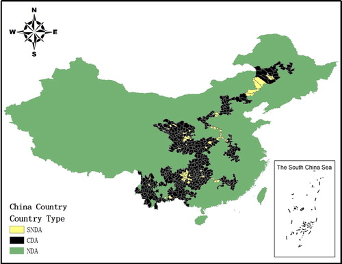
In Figure 1, SNDA is the supplementary non-poverty counties, CDA is the China’s 11 CDAs, and NDA is other non-poverty areas. As we can see in Figure 1, by joining these supplementary areas, the entire CDAs is geographically connected.

In addition, because the 505 poor counties were set up in the year 2004 in Wudu District, Longnan City, and Linxiang District, Lincang City, we employ a regression framework using a data-set of 573 counties in China, covering the period 2005–2012. There are two main types of data sources in this paper: one is the official statistical yearbook for 2,488 counties in China, including China Statistical Yearbook for Regional Economics 2006-2013, China Statistical Yearbook 2006-2013. The other is the sources of missing data, including Shaanxi, Gansu, Qinghai, Ningxia, Henan, Hubei, Chongqing, Sichuan, Hunan, Guizhou, Yunnan, Guangxi, Inner Mongolia, Jilin, Heilongjiang, Hebei, Shanxi, Anhui and Jiangxi, the data of counties in these 19 provinces are from their statistical yearbooks (2006-2013), respectively. Therefore, all the data in this article are derived from the official statistics released by China.

It should be noted that according to the China’s official statistics, there is no the data such as population density directly published by WDI at the county level. Except for the per capita GDP of the county, other indicators are obtained by the author according to the officially published material or data. Specifically, with reference to Fan and Xie (2014), per capita savings (yuan/person) is obtained by using the Balance of Saving Deposit of Households (10,000 yuan) divide by the Total Population of Household Registration (10000 Persons). The medical conditions and per capita income levels refer to the practice of Cheng et al. (2014), i.e. the number of beds in health care institutions divided by the total registered population. The per capita income level comes directly from China Statistical Yearbook (2006-2013). According to Zhang et al. (2013), the per capita education level is the substitution variable of the total number of students in middle schools and primary schools, while the per capita arable land is measured by the common cultivated land area of the poverty-stricken counties dividing by the total registered population. The urbanization rate is based on the practice of Zhang and Feng (2016), expressed as the proportion of non-agricultural population to the total population. Finally, the population density is measured by the total registered population (10,000 people) dividing by the administrative area (square kilometers). Table 1 shows the calculation method and information for indicators.

Table 1. The calculation method and information for indicators.

Full name of variable	Calculation method	Reference
per capita savings	$\mathit{saving}=\frac{\mathit{Balance\hspace{0.5em}}\mathit{of\hspace{0.5em}}\mathit{Saving\hspace{0.5em}}\mathit{Deposit\hspace{0.5em}}\mathit{of\hspace{0.5em}}\mathit{Households}(10000\mathit{yuan})}{\mathit{Total\hspace{0.5em}}\mathit{Population\hspace{0.5em}}\mathit{of\hspace{0.5em}}\mathit{Household\hspace{0.5em}}\mathit{Registration}(10000\mathit{Persons})}$	Fan and Xie (2014)
log per capita income	ln gdp	Cheng et al (2014)
number of beds per registered population	$\mathit{perbed}\frac{\mathit{Number\hspace{0.5em}}\mathit{of\hspace{0.5em}}\mathit{beds\hspace{0.5em}}\mathit{in\hspace{0.5em}}\mathit{health\hspace{0.5em}}\mathit{care\hspace{0.5em}}\mathit{institutions\hspace{0.5em}}(\mathit{piece}\mathit{of}\mathit{bed})}{\mathit{Total\hspace{0.5em}}\mathit{Population\hspace{0.5em}}\mathit{of\hspace{0.5em}}\mathit{Household\hspace{0.5em}}\mathit{Registration\hspace{0.5em}}(10000\mathit{Persons})}$	Cheng et al (2014)
population density	$\mathit{dpop}=\frac{\mathit{total\hspace{0.5em}}\mathit{population\hspace{0.5em}}(\mathit{person})}{\mathit{Poor\hspace{0.5em}}\mathit{county\hspace{0.5em}}\mathit{land\hspace{0.5em}}\mathit{area\hspace{0.5em}}(\mathit{square\hspace{0.5em}}\mathit{Kilometer})}$	Barbier and Hochard (2018)
per capita arable land	$\mathit{pcland}=\frac{\mathit{Common\hspace{0.5em}}\mathit{cultivated\hspace{0.5em}}\mathit{area\hspace{0.5em}}(\mathit{square\hspace{0.5em}}\mathit{Kilometer})}{\mathit{total\hspace{0.5em}}\mathit{population\hspace{0.5em}}(\mathrm{10000\hspace{0.5em}}\mathit{person})}$	Qin and Zhang (2016）
per capita education level	$\mathit{psacp}=\frac{\begin{array}{c}N\mathit{umber\hspace{0.5em}}\mathit{of\hspace{0.5em}}\mathit{students\hspace{0.5em}}\mathit{in\hspace{0.5em}}\mathit{general\hspace{0.5em}}\mathit{Secondary\hspace{0.5em}}\\ S\mathit{chool\hspace{0.5em}}\mathit{and\hspace{0.5em}}\mathit{ordinary\hspace{0.5em}}\mathit{primary\hspace{0.5em}}\mathit{Schools\hspace{0.5em}}(\mathit{person})\end{array}}{\mathit{Total\hspace{0.5em}}\mathit{Population\hspace{0.5em}}\mathit{of\hspace{0.5em}}\mathit{Household\hspace{0.5em}}\mathrm{Re}\mathit{gistration\hspace{0.5em}}(\mathrm{10000\hspace{0.5em}}\mathit{Persons})}$	Zhang et al (2013)
The urbanization rate	$\mathit{urban}=\frac{\mathit{Non}-\mathit{agricultural\hspace{0.5em}}\mathit{population\hspace{0.5em}}(\mathrm{10000\hspace{0.5em}}\mathit{person})}{\mathit{Total\hspace{0.5em}}\mathit{Population\hspace{0.5em}}\mathit{of\hspace{0.5em}}\mathit{Household\hspace{0.5em}}\mathit{Registration\hspace{0.5em}}(\mathrm{10000\hspace{0.5em}}\mathit{Persons})}$	Zhang and Feng (2016)

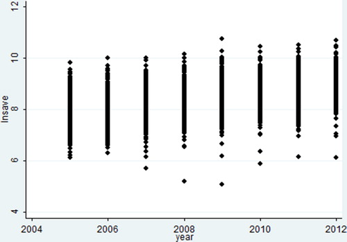
Figure 2 shows the change of per capita deposits (yuan) of the logarithmic value in CDAs from 2005 to 2012. It is easy to know that the per capita savings of the residents in the poverty-stricken areas not only show the characteristic of increasing year by year but also show the trend of gradual concentration and convergence. The reasons for the aforementioned characteristics and situations are undoubtedly multifaceted, such as economic growth, the improvement of medical condition, population density change, and urbanization promotion, et cetera. These effects of different factors on the situations in CDAs require further research and more in-depth identification through the use of spatial econometric regression methods.

Figure 2. The change of per capita deposits (yuan) of the logarithmic value in CDAs.

2.2. Theoretical mechanisms: the patterns of medical condition and population density affect residents’ savings in CDAs

It is argued that there is a significant positive correlation between income volatility and urban household saving rate (Shen & Xie, 2012). Zhu and Hang (2015) find that uncertainty in medical expenditures significantly enhances preventive savings motives for urban and rural residents, especially rural residents. Zhou and Wang (2018) concludes that contribution rate of medical insurance has a significant negative impact on the savings of rural residents. Bai, Li, and Wu (2012) find that medical insurance reduces preventive savings. However, it is not difficult to find out that the current conclusions on the relationship between medical stress and household savings are not well suited to explain the residents’ savings in CDAs. Because the situation in destitute areas are very different from other areas, the medical facilities in CDAs are generally lagging behind, if the number of hospitals and the number of per capita beds are scarce, the inhabitants living in hardship are likely to cope with the diseases all by themselves. Therefore it will further reduce their incomes and precautionary savings. On the contrary, with the improvement of the medical condition and services in CDAs, the local residents’ access to medical treatment is improved, and their willingness to seek medical treatment will increase, thus enhancing their preventive savings.

Regarding population, although many scholars have studied the household savings from the perspective of population structure based on the theory of life cycle, it could not make a reasonable explanation of the savings behavior of the residents in CDAs as well. Because the living standard of the residents is generally low, regardless of the age of the members of the poor families, they face more pressure to save due to their children’s education and family expenses. Actually, the population density may be more suitable for the analysis of residents’ savings behavior in CDAs. Since the labor force is the basic element of economic development, whereas in the destitute areas there are often sparsely populated and the population density is generally low. With the increase in population density in CDAs the economic activity will also increase, and the opportunities for entrepreneurship and investment will increase, thus allowing the residents of the region to increase their consumption, thereby reducing their savings.

Particularly, in China’s CDAs, not only the improvement of the medical condition and the increase of the population density will have obvious spatial dependency and spatial correlation, but also the interaction between the medical condition and the population density would have impacts on the savings of residents of the target CDAs and their neighborhood by means of spatial externalities. The improvement of the medical condition in CDAs helps to improve the living conditions of the local population and prolong their life expectancy, thereby attracting more people to move in, thus increasing the population density in this region. On the one hand, the increase in the proportion of the “unproductive” elderly population tends to curb savings (Yang & Zhang, 2013). Besides, the increase in the labor force can stimulate the economy and open up the local residents’ investment channels, then reduce residents’ precautionary savings motives.

On the other hand, the increase in population density will increase the demand for medical services, and with the existing level of medical services and established medical condition, the difficulty of seeing a doctor will be increasing. Thus, the medical condition in the CDAs will become relatively worse, and CDA residents who are ill will give up on themselves, which could weaken their precautionary savings motivation.

3. Model, method, and data

3.1. Model and method

The spatial econometric regression models are widely used because they take into account the spatial correlation and spatial dependence between different regions to varying degrees. Vega and Elhorst (2015) have discussed the internal relations among a variety of different forms of spatial models from the perspective of a general nesting spatial (GNS) model. The GNS model takes following form: (1) $$\mathbf{Y}=\rho \mathbf{WY}+\alpha {\mathbf{I}}_{\mathbf{N}}+\mathbf{X}\beta +\mathbf{WX}\theta +\mathbf{u},\mathbf{u}=\lambda \mathbf{Wu}+\mathbf{\epsilon },$$(1) where Y represents the dependent variable vector, W is a spatial weights matrix, I is an N × 1 vector of ones associated with the constant term parameter α, and X denotes an N × K matrix of explanatory variables associated with the K × 1 parameter vector β. The scalar parameters ρ and λ measure the strength of dependence between units, while β, like θ, is a K × 1 vector of response parameters. ε is a vector of independently and identically distributed disturbance terms, ε∼iid (0, σ_ε²I). Therefore, WY denotes the endogenous interaction effects, WX is the exogenous interaction effects, and Wu is the interaction effects. These endogenous and exogenous interactions reflect the spatially related effects of other regions’ variable changes on related variables in the target area and are an important aspect of reflecting spatial correlation.

Based on GNS, Vega and Elhorst (2015) analyzed the spatial Durbin model (SDM), spatial error model (SEM), spatial Durbin error model (SDEM), spatial autoregressive model (SAR), spatial autoregressive combined model (SAC), and spatial lag of X model (SLM). The SAR, SEM, and SLX models are special cases of SDM. After considering spatial correlation and spatial dependence, scholars define the exogenous effects comes from a change of a particular explanatory variable in a particular unit on its own dependent variable as direct effect (Vega & Elhorst, 2015), and define the exogenous effect comes from a change of a particular explanatory variable in a particular unit on the dependent variable of other contiguity unit as indirect effect (LeSage & Pace, 2009). SDM not only has advantages over SEM, SLX, and even SAR when capturing direct effects and indirect effects (Elhorst, 2010; Vega & Elhorst, 2015), but also it has been widely used to analyze endogenous interactions and exogenous interactions (LeSage & Pace, 2009; Elhorst, 2010). However, because GNS covers a variety of special forms of different spatial metrological regression models, it should be theoretically superior to SDM and other spatial econometric models. Therefore, we will focus on regression results of GNS for convenience. However, for the sake of robustness, it is necessary to examine the regression results of SAC, SLX, SDEM, and SDM. In particular, the regression coefficients of spatial econometric models should be explained from the perspectives of direct effect, indirect effect, and total effect (Xu, 2016).

Take expectations for Equation (1)(1) $$\mathbf{Y}=\rho \mathbf{WY}+\alpha {\mathbf{I}}_{\mathbf{N}}+\mathbf{X}\beta +\mathbf{WX}\theta +\mathbf{u},\mathbf{u}=\lambda \mathbf{Wu}+\mathbf{\epsilon },$$(1) , we get E(Y), then the matrix of partial derivatives of E(Y) with respect to the kth explanatory variable of X in unit 1 up to unit N has the following form: (2) $$\left[\frac{\partial E(\mathbf{Y})}{\partial x_{1k}}\dots \frac{\partial E(\mathbf{Y})}{\partial x_{\mathit{Nk}}}\right]={(\mathbf{I}-\rho \mathbf{W})}^{-1}\left[\begin{array}{cccc}{\beta }_k& W_{12}{\theta }_k& \cdots & W_{1N}{\theta }_k\\ W_{21}{\theta }_k& {\beta }_k& \cdots & W_{2N}{\theta }_k\\ ⋮& ⋮& ⋮& ⋮\\ W_{N1}{\theta }_k& W_{N2}{\theta }_k& \cdots & {\beta }_k\end{array}\right]$$(2) where ${(\mathbf{I}-\rho \mathbf{W})}^{-1}=\mathbf{I}+\rho \mathbf{W}+{\rho }^2{\mathbf{W}}^2+\cdot \cdot \cdot .$

The direct effects are represented by the mean value of diagonal elements in Equation (2)(2) $$\left[\frac{\partial E(\mathbf{Y})}{\partial x_{1k}}\dots \frac{\partial E(\mathbf{Y})}{\partial x_{\mathit{Nk}}}\right]={(\mathbf{I}-\rho \mathbf{W})}^{-1}\left[\begin{array}{cccc}{\beta }_k& W_{12}{\theta }_k& \cdots & W_{1N}{\theta }_k\\ W_{21}{\theta }_k& {\beta }_k& \cdots & W_{2N}{\theta }_k\\ ⋮& ⋮& ⋮& ⋮\\ W_{N1}{\theta }_k& W_{N2}{\theta }_k& \cdots & {\beta }_k\end{array}\right]$$(2) , while the indirect effects or spillover effects are represented by the mean value of off-diagonal elements in Equation (2)(2) $$\left[\frac{\partial E(\mathbf{Y})}{\partial x_{1k}}\dots \frac{\partial E(\mathbf{Y})}{\partial x_{\mathit{Nk}}}\right]={(\mathbf{I}-\rho \mathbf{W})}^{-1}\left[\begin{array}{cccc}{\beta }_k& W_{12}{\theta }_k& \cdots & W_{1N}{\theta }_k\\ W_{21}{\theta }_k& {\beta }_k& \cdots & W_{2N}{\theta }_k\\ ⋮& ⋮& ⋮& ⋮\\ W_{N1}{\theta }_k& W_{N2}{\theta }_k& \cdots & {\beta }_k\end{array}\right]$$(2) . However, the direct effects and indirect effects in different model specifications are different. In SAC, the direct effect is diagonal elements of (I-ρW)⁻¹β_k, and indirect effect is off-diagonal elements of (I-ρW)⁻¹β_k. In SLX/SDEM, the direct effect is β_k, and indirect effect is θ_k. While in GNS/SDM, the direct effect is the diagonal elements of (I-ρW)⁻¹(β_k+Wθ_k), and indirect effect is off-diagonal elements of (I-ρW)⁻¹(β_k+Wθ_k).Unlike exogenous interactions and endogenous interactions, direct and indirect effects are another important dimension used to describe spatial associations in spatial econometric regression models.

The spatial econometric regression models identify the spatial correlation by setting a spatial weight matrix. Therefore, the setting of the spatial weight matrix is the premise of constructing the spatial econometric regression models, and it is the key to capturing the spatial correlation between different regions. In the aspect of spatial weighting matrices, the binary contiguity matrix and the inverse distance weight matrix are widely used, in which w_ij is element (i, j) of the N × N spatial weight matrix W. In the binary contiguity weighting matrix, if two units share a common border, then the element w_ij = 1; otherwise w_ij = 0. In the inverse distance matrix, the element w_ij in the spatial matrix are assigned according to the following rules: $$w_{\mathit{ij}}=\{\begin{array}{c}1/d,i\ne j\hfill \\ 0,i=j\hfill \end{array},$$ where d is the Euclidean distances calculated from the latitude and longitude of each county. These two types of spatial weight matrices are the most commonly used, so we mainly use these two spatial weight matrices in the later analysis.

3.2. Data and spatial correlation test

3.2.1. Variables and data

On the basis of research on preventive savings (Starr-McCluer, 1996; Engen & Gruber, 2001) and Equation (1)(1) $$\mathbf{Y}=\rho \mathbf{WY}+\alpha {\mathbf{I}}_{\mathbf{N}}+\mathbf{X}\beta +\mathbf{WX}\theta +\mathbf{u},\mathbf{u}=\lambda \mathbf{Wu}+\mathbf{\epsilon },$$(1) , we get following spatial econometric equation: (3) $$\mathbf{ln}\mathit{save}=\rho ({\mathbf{I}}_{\mathbf{T}}\otimes {\mathbf{W}}_{\mathbf{N}})\mathbf{ln}\mathit{save}+\alpha {\mathbf{I}}_{\mathbf{NT}}+\mathbf{X}\beta +({\mathbf{I}}_{\mathbf{T}}\otimes {\mathbf{W}}_{\mathbf{N}})\mathbf{X}\theta +\mathbf{\epsilon },\mathbf{\epsilon }=\lambda \mathbf{W}\mathbf{\epsilon }+\nu$$(3) where save is per capita savings, $\otimes$ represents the Kronecker product, v ∼iid (0, σ_ε²I), and the remaining variables have the same meanings as described earlier. The vector of explanatory variables X including per capita GDP (gdp); per capita number of beds (perbed); population density (dpop); per capita arable land (pcland); the proportion of primary school students in average population, namely per capita education level (dpsacp); and the proportion of urban population in the total population (urban). We use perbed to measure the availability of medical condition in CDAs. Considering the availability of data, it is reasonable to believe that the number of beds per person can better measure the medical availability of the particularly poor areas, where the medical condition is relatively backward. Because the more beds per person in the hospital, it is more convenient to see a doctor in this area. This reflects an improvement in the medical condition in the region.

In order to mitigate the heteroskedasticity problem, all variables take the form with natural logarithms. In particular, to capture the interaction between the medical condition and population density, we introduce their cross-term (lnbed_lndpop). As mentioned before, an increase in population density in CDAs will increase medical demand, which in turn will make the original medical resources more scarce, and thus increase the difficulty of hospitalization for residents in CDAs.

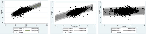
From the scatter plot of lnsave and lngdp (the left one in Figure 3), lnsave and lnperbed (the middle one in Figure 3) as well as lnsave and lndpop (the right one in Figure 3) we know that lngdp, lnperbed, and lndpop have a clear linear relationship with lnsave, especially the left and middle figures. This means that the regression coefficients of lngdp and lnperbed may be much more significant than the coefficient of lndpop.

Figure 3. The scatter plot of different variables.

3.2.2. Spatial correlation test

Before estimating the model, it is usually necessary to use the Moran’s I statistic to test the global spatial correlation of the variables. The Moran’s I statistic takes the form: (4) $$\mathit{Moran}’sI=\frac{{\sum }_{i=1}^n{\sum }_{j=1}^n{W}_{\mathit{ij}}(Y_i-\overline{Y})(Y_j-\overline{Y})}{S^2{\sum }_{i=1}^n{\sum }_{j=1}^n{W}_{\mathit{ij}}}$$(4) where $S^2=\frac{1}{n}{\sum }_{i=1}^n(Y_i-\overline{Y}),$ $\overline{Y}=\frac{1}{n}{\sum }_{i=1}^n{Y}_i,$ $Y_i$ is the observation of the ith county (i = 1, 2, …, 573), and n denotes the total number of counties. If $-1\le \text{Moran}’\mathrm{s}I<0,$ it represents that the spatial correlation is negative; if $0<\text{Moran}’\mathrm{s}I\le 1,$ it represents that the spatial correlation is positive; if $\text{Moran}’\mathrm{s}I=0,$ it represents the spatial correlation does not exist. We usually identify the significance of Moran’s I by constructing a Z-statistic. The original hypothesis H₀ means there is no spatial correlation. The Z-statistic is expressed as follows: (5) $$Z(I)=\frac{I-E(I)}{\sqrt{\mathit{Var}(I)}}\sim N(0,1)$$(5) in this statistic, Var(I) in the denominator represents the variance, and E(I) in the numerator represents the mean value. If the Z value rejects the original hypothesis, there is a spatial correlation. Table 2 shows the Moran’s I values for all variables and for a single variable. As Table 2 shows, not only all variables but also each single variable has significant and positive spatial correlation, and all of them show a gradual increase in the trend. Meanwhile Most of the Moran’s I values are greater than 0.3. This indicates the objective existence of spatial correlation in CDAs. In other words, there is spatial dependence between variables in the CDAs of China, and variable changes in one region can have a significant and positive impact on variables in other regions. Thus we should use a spatial econometric regression models rather than ordinary regression models that do not consider spatial correlation.

Table 2. The Moran’s I values for all variables and for a single variable.

	all	lngdp	lnperbed	lndpop	lnbed_lndpop	lnpcland	lndpsacp	lnurban
2005	0.3472*** (14.7416)	0.3517*** (14.5814)	0.3868*** (16.0177)	0.3721*** (15.4489)	0.3868*** (16.0121)	0.3747*** (15.5759)	0.3545*** (14.7178)	0.4025*** (16.6565)
2006	0.3691*** (15.6491)	0.3636*** (15.0704)	0.3971*** (16.4411)	0.3847*** (15.9648)	0.3980*** (16.4750)	0.3904*** (16.2243)	0.3568*** (14.8176)	0.3859*** (15.9684)
2007	0.3809*** (16.1372)	0.3689*** (15.2912)	0.3799*** (15.7254)	0.3714*** (15.4202)	0.3786*** (15.6709)	0.3811*** (15.8393)	0.3482*** (14.4627)	0.3869*** (16.0105)
2008	0.3293*** (13.9832)	0.3559*** (14.7609)	0.3402*** (14.0902)	0.3718*** (15.4347)	0.3329*** (13.7885)	0.3838*** (15.9522)	0.3408*** (14.1524)	0.3957*** (16.3756)
2009	0.3383*** (14.3293)	0.3370*** (13.9754)	0.3723*** (15.3994)	0.3677*** (15.2672)	0.3672*** (15.1874)	0.3798*** (15.7827)	0.3347*** (13.9067)	0.3745*** (15.5000)
2010	0.3051*** (12.9649)	0.2894*** (12.0199)	0.3350*** (13.8647)	0.3083*** (12.8187)	0.3318*** (13.7334)	0.3212*** (13.3687)	0.2965*** (12.3322)	0.3291*** (13.6321)
2011	0.4019*** (17.0041)	0.4096*** (16.9634)	0.4429*** (18.3090)	0.4271*** (17.7155)	0.4305*** (17.7932)	0.4276*** (17.7558)	0.3910*** (16.2181)	0.4036*** (17.7976)
2012	0.4013*** (16.9491)	0.3882*** (16.0811)	0.4074*** (16.8425)	0.3948*** (16.3835)	0.4060*** (16.7829)	0.3961*** (16.4571)	0.3659*** (15.1771)	0.4101*** (16.9581)

Notes: (1) The t-test values are in parentheses. Significance at the 10, 5, and 1% are indicated by single, double, and triple asterisks, respectively. (2) We use matlab2017 software to get the results and organize them into tables.

4. Empirical results

4.1. Regression results under binary contiguity matrix

Table 3 shows the various spatial econometric models’ regression results of the time-space double fixed effect in the binary contiguity spatial weight matrix. It is easy to see that, although their regression results have some differences, they have strong robustness.

Table 3. Regression results with time-space double fixed effect under the binary contiguity matrix.

	SLX	SDM	SDEM	SAC	GNS
lngdp	0.1472*** (7.5239)	0.1469^***(7.1278)	0.1498^***(7.4426)	0.2046^***(8.0278)	0.1473^***(7.1488)
lnperbed	0.3816^***(5.5712)	0.3569^***(4.9462)	0.3731^***(5.3018)	0.3995^***(6.4242)	0.3575^***(4.8280)
lndpop	−0.1455^***(−4.3270)	−0.1435^***(−4.0500)	−0.1509^***(−4.2971)	−0.1343^***(−4.0994)	−0.1447^***(−4.0266)
lnbed_lndpop	−0.0494^***(−3.7417)	−0.0462^***(−3.3198)	−0.0479^***(−3.5432)	−0.0524^***(−4.4636)	−0.0461^***(−3.2961)
lnpcland	0.0537^***(2.7720)	0.0540^***(2.6486)	0.0522^***(2.6157)	0.0374^**(2.1203)	0.0054^***(2.6430)
lndpsacp	0.1128*** (4.4006)	0.1097*** (4.0643)	0.1111*** (4.1875)	0.1104*** (4.5941)	0.1099*** (4.0950)
lnurban	0.0011 (0.1520)	−0.0004 (−0.0500)	0.0011 (0.1485)	0.0047 (0.6483)	−0.0003 (−0.0354)
W×lngdp	0.0479 (1.5460)	0.0133 (0.4040)	0.0470 (1.3720)	—	0.0161 (0.3429)
W×lnperbed	0.3779^***(3.8204)	0.2895^***(2.7644)	0.3926^***(3.6205)	—	0.3007^**(2.0610)
W×lndpop	−0.1262^**(−2.2915)	−0.0752(−1.2939)	−0.0965(−1.5850)	—	−0.0754(−1.1159)
W×lnbed_lndpop	−0.0472^**(−2.4864)	−0.0378^*(−1.8873)	−0.0527^**(−2.5372)	—	−0.0396(−1.6381)
W×lnpcland	−0.0351(−1.2513)	−0.0350(−1.1865)	−0.0235(−0.7558)	—	−0.0335(−1.0960)
W×lndpsacp	0.0002 (0.0053)	−0.0229 (−0.5808)	0.0013 (0.0321)	—	−0.0209 (−0.4501)
W×lnurban	0.03049** (2.4527)	0.0293** (2.2379)	0.0324** (2.3330)	—	0.0298** (2.2119)
ρ	—	0.1913*** (10.0998)	—	0.3095*** (5.5293)	0.1747* (1.7928)
λ	—	—	0.1893*** (9.9586)	−0.1134* (−1.6844)	0.0244 (0.1233)
R^2	0.1055	0.9427	0.9410	0.9428	0.9426
LogL	2,042.4	2,086.7	2,084.6	2,069.4	2,086.7
time fixed effect	Yes	Yes	Yes	Yes	Yes
space fixed effect	Yes	Yes	Yes	Yes	Yes
Nobs	4,584	4,584	4,584	4,584	4,584

Notes: (1) The t-test values are in parentheses. Significance at the 10, 5, and 1% are indicated by single, double, and triple asterisks, respectively. (2) We use matlab2017 software to get the results and organize them into tables.

Firstly, the spatial correlation coefficients (ρ and λ) estimated by different spatial econometric models are all significant at the 1% significance level, and their R² values in most of the spatial regression models (except for SLX) are greater than 0.9. These facts again indicate the rationality and necessity of using spatial econometrics.

Secondly, in terms of the regression coefficients of each model, we can see that the coefficients of the logarithm of gdp (lngdp) and perbed (lnperbed) are both positive and statistically significant at the 1% level of significance. These results are consistent with the theory that households’ savings are not only relevant to their income levels, but also positively related to the degree of improvement in the medical condition as has been previously described. Because the income levels of these CDAs are originally low, when medical conditions and medical condition are scarce, they will not make a “saving for medical treatment” part of their savings plan.

When it comes to the coefficients of natural logarithms of dpop (lndpop) and bed_pop (lnbed_pop, namely the natural logarithms of the cross term bed_dpop), both of them are negative and very significant. Since the GNS model is more general and representative than other regression models, so we take GNS results for example. In GNS results, a 1% increase in population density decreases residents’ savings in CDAs by 0.1447%, and the impact of the cross-items of medical condition and population density (lnbed_pop) on residents’ savings is -0.0461 and significant at the 1% level. These findings show that the increase in population density not only would reduce residents’ savings through its own, but also has negative effect on residents’ savings through the way of medical condition. This means that as CDAs’ population density increases, the needs of medical condition will increase as well, which will cause the medical condition to be deteriorating relatively and the medical services become scarcer, thereby reducing households’ precautionary savings.

Among other explanatory variables, the coefficients of the logarithm of pcland (lnpcland) and dpsacp (lndpsacp) are both positive and significant at the 1% level, while the coefficients of the logarithm of urban (lnurban) is insignificant in all models. These results illustrate that the increase of per capita arable land and per capita education level will both improve residents’ saving level. The reason is that both the increase in per capita arable land and the increase in education per capita will help to raise income levels of people in destitute areas or enhance their ability to earn high incomes, and both of these will in turn help increase their savings.

Besides, the exogenous interaction effects show that both W ×lnperbed and W ×lnurban have positive and significant effects on household savings in the GNS model. These exogenous interaction effects mean that the improvement of the medical condition as well as the advancement of urbanization in other areas which have spatial relationships with this target area can significantly promote household savings in the target area. On the one hand, with the improvement of the medical condition in the surrounding areas, the willingness of saving money for medical treatment of the residents live in the target destitute areas will increase. On the other hand, the accelerating urbanization in the surrounding destitute areas can provide more employment opportunities for residents in the target destitute area, and thus raise their savings levels.

Table 4 shows the direct effects, indirect effects, and total effects of SDM, SAC, and GNS. Similar to the previous analysis, we mainly discuss the regression results of GNS. From direct effects we know that lngdp, lnperbed, lnpcland, and lndpsacp will affect the residents’ savings in the target area positively and significantly, while lndpop and lnbed_pop both have negative and significant effect on these target areas’ own savings. Furthermore, the indirect effects in GNS indicate that lnperbed and lnurban in the target area have remarkable and positive effect on the residents’ savings in its neighbor areas. At the same time, lndpop and lnbed_pop in the target area have a negative and significant influence on its neighbor areas’ savings. Therefore, under the combined effects of direct effects and indirect effects, the coefficients of lndpop and lnbed_pop in the total effects are both negative and significant, whereas the total effect of lnperbed is positively and significantly.

Table 4. The direct effects, indirect effects, and total effects under the binary contiguity matrix.

	SDM
	lngdp	lnperbed	lndpop	lnbed_pop	lnpcland	lndpsacp	lnurban
Direct effects	0.1493^***(7.7048)	0.3754*** (5.0968)	−0.1490^***(−4.1928)	−0.0487^***(−3.4134)	0.0517^**(2.6224)	0.1114*** (4.0048)	0.0013 (0.1634)
Indirect effects	0.0489(1.3761)	0.4215*** (3.6553)	−0.1236^*(−1.7615)	−0.0547^**(−2.4788)	−0.0300(−0.9302)	−0.0051 (−0.1110)	0.0352** (2.3602)
Total effects	0.1982^***(5.4102)	0.7969*** (6.4855)	−0.2726^***(−3.5084)	−0.1033^***(−4.4927)	0.0218(0.6378)	0.1062** (2.1416)	0.0365** (2.1642)
	SAC
	lngdp	lnperbed	lndpop	lnbed_pop	lnpcland	lndpsacp	lnurban
Direct effects	0.1535^***(8.1667)	0.4127*** (6.3591)	−0.1375^***(−3.9791)	−0.0543^***(−4.4148)	0.0383^**(2.1675)	0.1132*** (4.5903)	0.0046 (0.6066)
Indirect effects	0.0640^***(3.9479)	0.1723*** (3.6120)	−0.0574^***(−2.9246)	−0.0227^***(−3.0890)	0.0160^*(1.9259)	0.0472*** (3.1955)	0.0019 (0.5692)
Total effects	0.2176^***(7.5930)	0.5850*** (6.0066)	−0.1949^***(−3.8954)	−0.0770^***(−4.2846)	0.0543^**(2.1531)	0.1604*** (4.4696)	0.0066 (0.5999)
	GNS
	lngdp	lnperbed	lndpop	lnbed_pop	lnpcland	lndpsacp	lnurban
Direct effects	0.1498^***(7.2251)	0.3755*** (5.3183)	−0.1480^***(−4.1374)	−0.0486^***(−3.5775)	0.0518^**(2.5392)	0.1094*** (4.1351)	0.0014 (0.1839)
Indirect effects	0.0482(1.2067)	0.4264*** (3.1207)	−0.1242^*(−1.6920)	−0.0553^**(−2.1851)	−0.0278(−0.7892)	−0.0021 (−0.0449)	0.0353** (2.1298)
Total effects	0.1980^***(4.7703)	0.8019*** (5.7448)	−0.2772^***(−3.2987)	−0.1039^***(−4.0645)	0.0240(0.6396)	0.1074** (2.1032)	0.0367* (1.9731)

Notes: (1) The t-test values are in parentheses. Significance at the 10, 5, and 1% are indicated by single, double, and triple asterisks, respectively. (2) We use matlab2017 software to get the results and organize them into tables.

4.2. Regression results under inverse distance matrix

Table 5 presents the different spatial regression models of the time-space double fixed effect under inverse distance matrix. These results not only are similar with the results under the binary contiguity matrix in Table 3 but also are strongly robust. The spatial correlation coefficients (ρ and λ) in almost all of the spatial econometric models are significant at the 10% significance level, and most of R² values (except for SLX model) are greater than 0.9. The coefficients of the logarithm of gdp (lngdp) and perbed (lnperbed) are also both positive and statistically significant at the 1% level of significance.

Table 5. Regression results with time-space double fixed effect under inverse distance matrix.

	SLX	SDM	SDEM	SAC	GNS
lngdp	0.1443*** (6.7114)	0.1453^***(7.2987)	0.1435^***(7.2233)	0.1567^***(8.2664)	0.1443^***(7.2478)
lnperbed	0.4221^***(6.3492)	0.4076^***(5.7663)	0.4141^***(5.8621)	0.3999^***(6.0539)	0.4129^***(5.8238)
lndpop	−0.1192^***(−3.6126)	−0.1190^***(−3.3933)	−0.1200^***(−3.4243)	−0.1281^***(−3.7496)	−0.1193^***(−3.3996)
lnbed_pop	−0.0598^***(−4.6719)	−0.0575^***(−4.2219)	−0.0584^***(−4.2877)	−0.0535^***(−4.2407)	−0.0583^***(−4.2745)
lnpcland	0.0729^***(3.8810)	0.0726^***(3.6371)	0.0732^***(3.6672)	0.0525^**(2.7900)	0.0730^***(3.6578)
lndpsacp	0.1185*** (4.7050)	0.1194*** (4.4558)	0.1123*** (4.1970)	0.1185*** (4.6671)	0.1158*** (4.0950)
lnurban	−0.0050 (−0.6883)	−0.0049 (−0.6369)	−0.0035 (−0.4581)	0.0011 (0.1391)	−0.0042 (−0.5514)
W×lngdp	0.3470* (1.8854)	0.1361 (0.6932)	0.3768 (1.6394)	—	0.2620 (1.0904)
W×lnperbed	2.6190^***(5.0151)	1.7024^***(3.0471)	2.6568^***(4.0439)	—	2.1836^**(2.8997)
W×lndpop	−0.8146^**(−2.4275)	−0.4483(−1.2539)	−0.6606(−1.5362)	—	−0.6111(−1.4410)
W×lnbed_pop	−0.2617^***(−2.7896)	−0.1587(−1.5875)	−0.2685^**(−2.2663)	—	−0.2116^*(−1.7476)
W×lnpcland	−0.3970^**(−2.4492)	−0.3217^*(−1.8651)	−0.4234(−2.1010)	—	−0.3772^*(−1.9430)
W×lndpsacp	−0.5261*** (−2.7350)	−0.5231^**(−2.5575))	−0.3907 (−1.5835)	—	−0.4789** (−2.0829)
W×lnurban	0.4593** (5.5321)	0.3276*** (3.7020)	0.3592*** (3.4977)	—	0.3624*** (3.4820)
ρ	—	0.7623*** (14.9453)	—	0.8837*** (14.8127)	0.3549* (1.8102)
λ	—	—	0.8036*** (17.4323)	0.3980* (1.8136)	0.5468 (0.15923)
R^2	0.1255	0.9429	0.9423	0.9420	0.9426
LogL	2,094.2	2,106.6	2,106.6	2,068.4	2,108.3
time fixed effect	Yes	Yes	Yes	Yes	Yes
space fixed effect	Yes	Yes	Yes	Yes	Yes
Nobs	4,584	4,584	4,584	4,584	4,584

Notes: (1) The t-test values are in parentheses. Significance at the 10, 5, and 1% are indicated by single, double, and triple asterisks, respectively. (2) We use matlab2017 software to get the results and organize them into tables.

For the same reasons as mentioned previously, we only discuss the regression results of GNS. The coefficients of lnperbed, lndpop, and lnbed_pop in the GNS model are 0.4129, −0.1193, and −0.0583, respectively. All of them are negative and very significant, and these results are similar with the results in Table 3. Besides, other variables’ coefficients are also roughly equal to the coefficients in Table 3. Therefore, these results are robust.

Table 6 shows the direct effects, indirect effects, and total effects of SDM, SAC, and GNS. From these direct effects we know that lngdp, lnperbed, lnpcland, and lndpsacp will affect the residents’ savings in the target area positively and significantly, whereas lndpop and lnbed_pop both have negative and significant effect on this target area’ own savings. These results are almost the same with those in Table 3.

Table 6. The direct effects, indirect effects, and total effects under inverse distance matrix.

	SDM
	lngdp	lnperbed	lndpop	lnbed_pop	lnpcland	lndpsacp	lnurban
Direct effects	0.1478^***(7.8707)	0.42628^***(5.8831)	−0.1243^***(−3.5359)	−0.0595^***(−4.2472)	0.0692^**(3.5867)	0.1172*** (4.2367)	−0.0018 (0.2267)
Indirect effects	1.0700(1.2277)	8.7629*** (2.7567)	−2.4152(−1.3469)	−0.8775^*(−1.8311)	−1.1811(−1.5006)	−1.95358* (−1.8413)	1.4172*** (2.7809)
Total effects	1.2178(1.4007)	9.1892*** (2.8960)	−2.5395(−1.4162)	−0.9370^*(−1.9653)	−1.1119(−1.4183)	−1.8364* (−1.7351)	1.4154** (2.7764)
	SAC
	lngdp	lnperbed	lndpop	lnbed_pop	lnpcland	lndpsacp	lnurban
Direct effects	0.1597^***(6.4211)	0.4097*** (5.3196)	−0.1300^***(−3.4546)	−0.0550^***(−3.9365)	0.0535^**(2.7047)	0.1205*** (4.2799)	0.0009 (0.1086)
Indirect effects	1.5993(0.1860)	3.9324 (0.1904)	−1.3181(−0.2045)	−0.5212(−0.1812)	0.5508(0.1685)	1.1908 (0.1902)	0.0129 (0.0298)
Total effects	1.7590(0.2042)	4.3421 (0.2098)	−1.4481(−0.2242)	−0.5762(−0.1999)	0.6043(0.1844)	1.3114 (0.2091)	0.0138 (0.0316)
	GNS
	lngdp	lnperbed	lndpop	lnbed_pop	lnpcland	lndpsacp	lnurban
Direct effects	0.1455^***(6.7724)	0.4204*** (4.9984)	−0.1197^***(−3.2387)	−0.0593^***(−4.1191)	0.0714^***(3.4387)	0.1141*** (4.1295)	−0.0030 (−0.2984)
Indirect effects	0.3675(0.0928)	3.8744 (0.1410)	−1.2933(−0.2089)	−0.3805(−0.1268)	−0.6235(−0.1918)	−0.8797 (−0.1625)	0.5952 (0.1480)
Total effects	0.5131(0.1293)	4.2948 (0.1560)	−1.4130(−0.2278)	−0.4398(−0.1463)	−0.5521(−0.1695)	−0.7656 (−0.1412)	0.5922 (0.1469)

Notes: (1) The t-test values are in parentheses. Significance at the 10, 5, and 1% are indicated by single, double, and triple asterisks, respectively. (2) We use matlab2017 software to get the results and organize them into tables.

However, all of the coefficients in indirect effects and the total effects are insignificant in the GNS model. The finding here is different from the results in Table 4. The main reason may be that there is a difference in the construction methods of inverse distance spatial weight matrix and binary contiguity matrix, the spatial correlation effects they capture are inevitably different; therefore, the regression results in indirect effects based on these matrixes are different.

5. Conclusion

Using the spatial panel data of China’s 11 Contiguous Destitute Areas from 2005 to 2012 and the different kinds of econometric regression models, we estimate the effect of medical condition and population density on the residents’ savings in these 11 CDAs. Using coefficients from SEM, SLX, SAR, SAC, SDM, SDEM, and GNS model specifications, we find the results that the coefficients of lnperbed, lndpop, and lnbed_pop are roughly 0.4, −0.15, and −0.05, respectively. In most of these models, especially in the direct effects, indirect effects, and total effects, these results are roughly the same and robust. These findings mean that medical condition and population density not only have influence on residents’ savings on their own, but also will decrease the residents’ savings by their interaction effects. Besides, most of these variables in the model not only have direct effect on residents’ savings but also most of them have indirect effects on it. These results show that in China’s destitute areas, the impact of medical condition and population density on household savings is not only an interactive process, but also a process of spatial interaction and interdependence between different regions.

Our study offers empirical support for improving the residents’ well-being in CDAs. First and foremost, it is necessary and important to improve residents’ medical conditions, so that the sick people in CDAs can get timely medical treatment although they may cure their illness mainly by raising their precautionary savings rate. Besides, the improvement of medical condition will help to retain the local population or even to facilitate the flow of people from other areas, and then will reduce residents’ precautionary savings in CDAs. These will be beneficial to improving the development prospects in CDAs and revitalizing CDAs’ economies. Secondly, because of the differences of spatial weight matrix, we do not find significant impacts of indirect effects of the variables in GNS under the inverse distance spatial weight matrix, yet the indirect effects in the GNS model under binary contiguity matrix are much more significant and the spatial correlations do exist in China’s CDAs. Therefore, in China's poverty alleviation work, we should fully consider the spatial correlation between the various destitute areas and promote the poverty alleviation policies as a whole. Last but not least, excavate and carry forward the characteristics and comparative advantages of the destitute areas, encourage social capital to enter CDAs to develop characteristic industries, enhance the protection of cultivated land in the destitute areas and expand the construction of basic education facilities, thus promote CDAs’ economic growth through various channels.

The novelty of the paper lies in identifying the specific effects of medical condition and population density on the residents’ savings in China’s 11 CDAs by using the spatial econometric methods. So far, we have not seen any research using this method to study similar problems. Inevitably, there are still some shortcomings in this paper that needed further research. On one hand, the core variables in the regression results are not significantly promoted in all the estimation results, and the underlying causes of this result require further study. On the other hand, there are many factors affecting the savings level of poor residents, and the impact is complicated. Therefore,if the data is available, it is necessary to include more influencing factors into the scope of research, and to explore the comprehensive impact of different factors on the residents’ savings level in CDAs.

Disclosure statement

The authors reports no conflicts of interest.

Additional information

Funding

Phased achievements of Natural Science Foundation of Guangdong Province of China “Research on Guangdong Industrial Structure Adjustment Based on the Perspective of Demographic Dividend Transition” (2017A030310667), “Internet Economy and Regional Economic Growth and Convergence Research” (2018M641583), and “Research on the Deepening and Innovation of Regional Coordination Development Mechanism Based on Multipolar Network Space Organizations” (17AJL11).

Notes

1 http://ghs.ndrc.gov.cn/zcfg/index_1.html.

References

- Bai, C. E., Li, H. B., & Wu, B. Z. (2012). Health insurance and consumption: Evidence from China’s new cooperative medical scheme. Economic Research Journal (in Chinese), 64(2), 41–53.
- Barbier, E. B., & Hochard, J. P. (2018). Land degradation. Nature Sustainability, 1(11), 623–631. doi:10.1038/s41893-018-0155-4
- Carroll, C. D., & Kimball, M. S. (2001). Liquidity constraints and precautionary saving. NBER Working Paper No.8496. http://www.nber.org/papers/w8496.
- Cheng, M. W., Jin, Y. H., Cai, Q. E., & Shi, Q. H. (2014). Focusing on education or health improvement for anti-poverty in rural China: Evidence from national household panel data. Economic Research Journal (in Chinese), 2014(11), 132–144.
- Cosci, S., & Mirra, L. (2018). A spatial analysis of growth and convergence in Italian province: The role of road infrastructure. Regional Studies, 52(4), 516–527. doi:10.1080/00343404.2017.1334117
- Ding, J. J. (2014). Comparative analysis on poverty degree of China’s 11 contiguous destitute Areas: With view of comprehensive development index. Scientia Geographica Sinica (in Chinese), 34 (12), 1418–1427. doi:10.13249/j.cnki.sgs.2014.12.002
- Dollar, D., Kleineberg, T., & Kraay, A. (2016). Growth still good for the poor. European Economic Review, 81, 68–85. doi:10.1596/1813-9450-6568
- Elhorst, J. P. (2010). Applied spatial econometrics: Raising the bar. Spatial Economic Analysis, 5(1), 9–28. doi:10.1080/17421770903541772
- Engen, E. M., & Gruber, J. (2001). Unemployment insurance and precautionary saving. Journal of Monetary Economics, 47(3), 545–579. doi:10.1016/S0304-3932(01)00051-4
- Fan, L. M., & Xie, E. (2014). Do public transfers reduce vulnerability? Economic Research Journal (in Chinese), 2014(8), 67–78.
- Fang, L. M., & Qiao, D. P. (2012). The effect of the urban medical security system on the economic burden of access to health care on the urban poor: Based on the survey of the urban poor households in Bazhou, Chibi and Hechuan of China. Journal of Finance and Economics (in Chinese), 2012(11), 103–113. doi:10.16538/j.cnki.jfe.2012.11.012
- Gong, W. J., Qin, C. L., & Li, C. (2018). Poverty alleviation effect of China’s Fiscal expenditure – Based on structure and space. Research on Economics and Management (in Chinese), 39 (5), 24–37. doi:10.13502/j.cnki.issn1000-7636.2018.05.003
- Hu, C., & Xu, Z. Y. (2014). Empirical analysis on the population ageing and saving rate: The data from Chinese families. China Economic Quarterly (in Chinese), 2014(4), 1345–1364.
- Huang, X. J., & Wu, C. F. (2006). The crowding out effect of social health insurance on precautionary saving. The Journal of World Economy (in Chinese), 2006(8), 65–70.
- Husmann, C. (2016). Marginality as a root cause of poverty: marginality hotspots in Ethiopia. World Development, 78(2), 420–435. doi:10.1016/j.worlddev.2015.10.024
- Leland, H. E. (1968). Saving and uncertainty: The precautionary demand for saving. The Quarterly Journal of Economics, 82(3), 465–473. doi.10.1016/B978-0-12-214850-7.50014-0 doi:10.2307/1879518
- LeSage, J. P., & Pace, R. K. (2009). Introduction to spatial econometrics. Boca Raton. FL: Taylor and Francis.
- Menegatti, M. (2007). A new interpretation for the precautionary saving motive: A note. Journal of Economics, 92(3), 275–280. doi:10.1007/s00712-007-0279-x
- Nándori, E. S. (2014). The role of economic growth and spatial effects in poverty in Northern Hungary. Regional Statistics, 4, 28–39. doi:10.15196/RS04103
- Peng, X. L., & Yuan, J. X. (2008). An analysis of peasants’ preventive savings for uncertainties in poor minority areas: A case from Wuling Mountains. Consumer Economics (in Chinese), 24(2), 38–40.
- Qin, Y., & Zhang, X. B. (2016). The road to specialization in agricultural production: evidence from rural China. World Development, 77(1), 1–16. doi:10.1016/j.worlddev.2015.08.007
- Shen, K. R., & Xie, Y. (2012). The empirical research on the uncertainty and the household savings rate in urban China. Journal of Financial Research (in Chinese), 2012(3), 1–13.
- Starr-McCluer, M. (1996). Health insurance and precautionary saving. American Economic Review, 86(1), 285–295.
- Tang, J., Yu, J. W., & Rao, C. (2014). Return-migration willingness of temporary migrants and household savings behaviors within the dual structure in China: Evidence from dynamic monitoring data of temporary migrant in Beijing, Shanghai and Guangzhou in 2012. Journal of Finance Research (in Chinese), (12), 23–38.
- Vega, S. H., & Elhorst, J. P. (2015). The SLX model. Journal of Regional Science, 55(3), 339–363. doi:10.1111/jors.12188
- Xu, C. H. (2016). The tendency of general rate of profit to fall in post-crisis era: Performance, national differences and influencing factors. The Journal of World Economy (in Chinese), (5), 3–28.
- Yang, J. J., & Zhang, E. Z. (2013). The effects of the age structure of population and the old-age insurance system transition on residents’ savings rates. Social Sciences in China (in Chinese), (8), 47–66.
- Zhang, S. B., & Feng, F. (2016). Poverty reduction effect of rural worker’s urbanization in rural place of Guizhou. Economic Geography (in Chinese), 36(11), 141–145. doi:10.15957/j.cnki.jjdl.2016.11.019
- Zhang, Y., Wan, G. H., & Shi, Q. H. (2013). Chronic poverty and transient poverty in rural China: decomposition and their determinants. Economic Research Journal (in Chinese), 2013(4), 119–129.
- Zhang, J. L., & Yan, D. D. (2016). Multi-dimensional endowment conditions, geographical spatial spillover and regional poverty governance. Chinese Journal of Population Science (in Chinese), 32(5), 35–48.
- Zhou, Y., & Wang, G. J. (2018). Population structure, medical insurance and high residential savings from the perspective of urban and rural differences. Journal of Capital University of Economics and Business (in Chinese), 20(3), 13–20. doi:10.13504/j.cnki.issn1008-2700.2018.03.002
- Zhu, B., & Hang, B. (2015) Liquidity constraints, health expenditure and precautionary saving: An empirical research based on China’s provincial panel data. Macroeconomics (in Chinese), 2015(3), 112–119 + 133. doi:10.16304/j.cnki.11-3952/f.2015.03.014
- Zhu, C., Zhou, Y., & Zhang, L. J. (2012). Demographic effects on savings, investments and external balance: Evidence from Asia. Chinese Journal of Population Science (in Chinese), 2012(1), 39–50.
- Zou, W., & Zheng, H. (2014). Why kids from poor families don’t study? Risk, intergenerational transmission of human capital and poverty traps. Economic Perspectives (in Chinese), 2014(6), 16–31.