Ricardian model theory under different transfer forms and input factors

Abstract

Desmet and Ortín analysed regional development using a Ricardian model theory. This paper uses their framework. The authors analyse the influence of wage subsidization, unemployment benefit, public employment management, consideration of the demographic factor and asymmetric value of the input factor labor on the development of regional inequalities between regions. By reducing the labor in the Ricardian model framework, the input factor can be reduced. The lower input factor labor leads to a reduction in the world market supply and to lower production, which in turns to decline in prosperity. Practical relevance results from the effects of external shocks such as unemployment benefits or demographic aspects. Both aspects reduce the labor population (asymmetric distribution of the input factor labor). This damages the advanced region rather than the underdeveloped region.

Keywords:

• Regional economic disparities
• Ricardian model theory
• transfer forms
• Development
• Environmental Issues and Changes

JEL CLASSIFICATIONS:

• F11
• O11
• R11

1. Introduction

The authors Aghion, Bertola, Hellwig, Pisani-Ferry, Rosati, Sánchez Bajo, Sapir, Vinals and Wallace examined regional development in Europe from 1970 to 1998. Although regional inequality fell by 50 percentage points between 1970 and 1998 and the reduction in inequality was deemed to have been resolved, the picture today is different. At present, regional inequality is returning to the benefit level of 1970 (Sánchez Bajo, 2007, p. 36; Sapir et al., 2004, p. 79).

Authors explain regional development (Desmet & Ortín, 2007; Gumpert, 2019a, 2019b). Desmet and Ortín focus exclusively on utility levels under a Ricardian model framework. Gumpert further develops the statements on regional development and transfers the individual period patterns to the Heckscher–Ohlin theorem, to the core peripheral model, and to a newly developed extended core peripheral model. The effects of the different model-dependent influence possibilities are analysed by external shocks such as input factors, production functions, relative price or economies of scale.

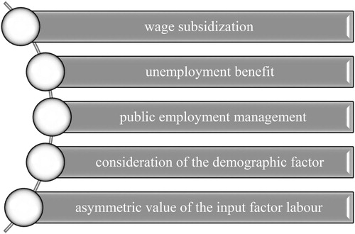
Consequently, a large number of analyses with different model frameworks are available. It is more interesting to consider how external shocks impact one another. The aim of this paper is to examine how external shocks affect inequality between regions. The following are regarded as external shocks: wage subsidization, unemployment benefit, public employment management, consideration of the demographic factor and asymmetric value of the input factor labour. Figure 1 illustrates the individual influencing factors examined in this paper.

Figure 1. Influencing factors. Author’s illustration.

The question arises as to whether such measures can strengthen the convergence process and restore economic convergence.

The authors Boltho, Brunello, Carlin, Faini, Lupi, Ordine, Paci, Saba and Scaramozzino noted that the change in policy and the monetary support associated with it led to a reduction in regional inequality (Boltho, Carlin, & Scaramozzino, 1997; Paci & Saba, 1998). The regions approached each other over the considered periods (Brunello, Lupi, & Ordine, 2001, p. 104; Faini, 1995). As a result, between 1971 and 1990, wage income per person increased by 23.00% more in the underdeveloped South than in the North (Desmet & Ortín, 2007, p. 1). This represents a reduction in regional inequality.

The lack of identical growth in labor productivity over time made Southern Italy less attractive for new technologies. As a result, the regional reduction to a fixed level has been affected and fluctuates only marginally. Table 1 illustrates these statements. As a result, the financial transfers could no longer force further economic convergence. Between 2013 and 2016, there were no significant changes in relative regional development despite monetary transfers.

Table 1. Periodic analysis of GDP for Italy.^a

Year	GDP: Northern and Central Italy (million €)	Share: Northern Italy to Central Italy (in %)	GDP: Southern Italy (million €)	Share: Southern Italy (in %)
2013	1,251,635.00	77.77	242,519.00	15.07
2014	1,241,906.00	76.96	249,955.00	15.49
2015	1,268,533.00	77.09	255,557.00	15.53
2016	1,296,641.00	77.16	262,189.00	15.60

^a Author’s illustration – Eurostat 2015, p. 7; Eurostat, 2016, p. 6; Eurostat, 2017, p. 6; Eurostat, 2018, p. 6).

This raises the question of why, despite the financial transfers, there is no further rapprochement between the regions. Factors such as population density, population growth or net migration tend to lead to divergence (Desmet & Ortín, 2007; Gumpert, 2013). The question now is how the new possibilities of influence, such as unemployment benefits or public employment, affect regional development and whether this in turn increases/improves convergence.

The analysis of the migration balance also clearly shows an increase in asymmetric behavior in the expression of input factors in Northern, Central and Southern Italy. The employment and unemployment rates in turn influence the input factors for the production of goods, but also the ancillary costs for social benefits, the state budget and unemployment benefit levels. These counteracting factors influence regional developments indirectly rather than directly via financial transfers. However, the monetary transfer levels can be used as a measurement variable in the analysis.

2. Background to the model

This article contributes to the literature about the development behavior of regions. Two regions and their possible developments are considered. The focus is on full specialization. In the economy of Italy or Germany, many support options, such as wage subsidies are permitted within a region. Furthermore, the regions must manage various problems such as demographics (Martin & Sunley, 2017; Paci & Saba, 1998; Pflüger, 2007, p. 1).

Figure 1 illustrates the individual influencing factors examined in this paper. Wage subsidies are suitable in the model. When applied to economic development, the use of wage subsidies is a common tool in areas in Germany. In some areas, wages are subsidized for existing productivity (e.g., in agriculture) to maintain the factor rate in the region. This adjustment is important for preventing ‘bleeding’ of the regions. This disadvantage of wage subsidies is that this form of transfer makes the underdeveloped region less active. If no sustainable growth effect is triggered, long-term development and development leaps disappear (Fonseca, 2017, p. 28; Sinn, 2000, p. 120; Sinn & Westermann, 2001, p. 19).

Unemployment benefits were also built into the model. As the first step, the Cobb–Douglas utility function must be adapted because of the case decision between ‘employment’ and ‘no employment’. The workers can choose between these two conditions or may be forced into these two situations. The parameters are subsequently selected in such a manner that at least one consumer has an incentive to become unemployed in the underdeveloped South. In the labor market of the underdeveloped South, an equilibrium is achieved when agricultural workers and the unemployed enjoy the same benefits. Due to the higher wages in the advanced region than in the underdeveloped South, no worker in the production of industrial goods will have an incentive to move into the agricultural sector. Similarly, no industrial worker will have an incentive to become unemployed, because incomes are identical in the agricultural sector and unemployment (Boschma & Frenken, 2017, p. 214; Demko, 2017, p. 68; Hanusch, Kuhn, & Cantner, 2002; IWH, 2004; Karl, Möller, & Wink, 2003; Ludwig, 2004).

The public administration is strong in every country. The administration has statutory tasks, implements policy objectives, provides services to society, and intervenes in active life to shape processes and procedures for citizens. Only well-organized public employment can guarantee a functioning economy (Demmke, 2005, p. 7; Ehrenfeld, 2004; Haensch & Holtmann, 2008, p. 606; Pindyck & Rubinfeld, 2003).

Since 2011, Germany's population has been approximately 81.5 million inhabitants. Since the 1950s, 12 million more people are living in Germany. This increase has been intermittent and unsteady (Annual Report of the Federal Government, 2004; Just, 2013, p. 9).

The peak in population growth was in 2005, with 82.5 million people, followed by a steady decline in the number of inhabitants. Due to the reduced birth rate and lack of young immigration, the proportion of young people in the total population is steadily decreasing. Furthermore, the existing population continues to age. This effect is intensified by people getting older. The decrease in the birth rate depends on three factors (Just, 2013, p. 12; Krugman, Obstfeld, & Melitz, 2011; Leipert, 2003):

1. Number of women of childbearing age between 15 and 49 years.

2. Number of children a woman gives birth to on average.

3. Age at which women give birth to the first child.

In the model, ‘pensioners’ are defined as out-of-pocket employees who are no longer available to the labor market. The society comprising the young population has to increase the basic income (pension) for the pensioners. Consequently, the demographic effect will have a negative impact on society (Max Planck Institute for Demographic Research, 2014; Mueller, Nauck, & Diekmann, 2000; Padoa Schioppa & Basile, 2002; Samuelson & Nordhaus, 2005).

Another influencing factor is the different set of factors. In the case of Germany, for example, the population has been declining slightly for years. The input factor ‘work’ thus decreases slightly. In contrast, India’s population is increasing rapidly. Consequently, there is a higher input factor for labor. The higher input factors enable the area to move beyond backwardness. In the long term, problems occur from unbridled population growth and demography (Krugman & Venables, 1995; United Nations, 2017).

Finally, the financial transfers should be mentioned again. Financial transfers in the European Union flow into structurally weak regions through the Structural Funds, without any immediate consideration – like increases in productivity (Brezis & Tsiddon, 1998; European Commission, 2013a, 2013b, 2014).

3. The model

Desmet and Ortín argue that asymmetric learning effects explain unequal regional development (Boschma & Frenken, 2017, p. 214; Demko, 2017, p. 68; Gumpert, 2016). There are different learning effects and learning characteristics in the individual sectors, which results in differences in productivity between sectors. Equation (1)(1) $$L=L^{*}=1$$(1) defines the labor in the North and South in the Ricardian model theory. (1) $$L=L^{*}=1$$(1)

The labor per sector is marked with L in the Northern region and L* in the Southern region, with L_F and L_F* representing the agricultural sector and L_M and L_M* representing the industrial sector. The technology in the industrial sector is defined as A and A* for the Northern and Southern regions (first period). The industrial sector is characterized by a knowledge effect. There is no specific learning effect in the agricultural sector.

Wage subsidies Sub, unemployment benefits AU, public employment ÖB and demographics DG play a role in the Ricardian model theory in the North and South. Wage subsidization especially promotes the labor factor in the underdeveloped region, thus making fewer workers available in the North. In the South, by contrast, the factor will increase.

A similar picture is available for unemployment benefits, the public sector and demography. Fewer workers will be available. The unemployed and aged sections of the population are not available to the economy. People in the public sector are also not involved in the production of output goods. Equations (2)–(5) indicate the individual influencing factors of the advanced North, while Equation (6)(6) $$L_{M,\mathit{MOD}}=A_M\cdot \left(1-\eta -\varphi -\kappa -\Lambda \right)\cdot L_M$$(6) indicates the total input for the North. (2) $$L_{M,\mathit{Sub}}=\left(1-\eta \right)\cdot L_M$$(2) (3) $$L_{M,AU}=\left(1-\varphi \right)\cdot L_M$$(3) (4) $$L_{M,ÖB}=\left(1-\kappa \right)\cdot L_M$$(4) (5) $$L_{M,DG}=\left(1-\Lambda \right)\cdot L_M$$(5) (6) $$L_{M,\mathit{MOD}}=A_M\cdot \left(1-\eta -\varphi -\kappa -\Lambda \right)\cdot L_M$$(6)

Similarly, the individual components for the underdeveloped South can be represented, which is completely specialized in the agricultural sector according to the described derivation. In the event of subsidization, the number of workers is increased by wage structures. (7) $$L_{F,\mathit{Sub}}^{*}=L_F^{*}+\eta \cdot L_M$$(7) (8) $$L_{F,AU}^{*}=\left(1-{\varphi }^{*}\right)\cdot L_F^{*}$$(8) (9) $$L_{F,ÖB}^{*}=\left(1-{\kappa }^{*}\right)\cdot L_F^{*}$$(9) (10) $$L_{G,DG}^{*}=\left(1-{\Lambda }^{*}\right)\cdot L_F^{*}$$(10) (11) $$L_{F,\mathit{MOD}}^{*}=A_F^{*}\cdot \left(\left(1-{\varphi }^{*}-{\kappa }^{*}-{\Lambda }^{*}\right)\cdot L_F^{*}+\eta \cdot L_M\right)$$(11)

There is a Cobb–Douglas function, which is a special function of the CES function. This functional form is used in the analysis for consumers and companies (Cobb & Douglas, 1928). The production function for analyzing the model is defined below. The output is presented according to the patterns of specialization (Desmet & Ortín, 2007, p. 5; Ribhegge, 2007, p. 19; Siebert, 2000, p. 29; Sieg, 2007, p. 360). The authors summarise the contents of the input factor for the industrial and agricultural sectors with MOD. (12) $$Q_F^{*}=A_F^{*}\cdot \left(\left(1-{\varphi }^{*}-{\kappa }^{*}-{\Lambda }^{*}\right)\cdot L_F^{*}+\eta \cdot L_M\right)$$(12) (13) $$Q_M=A_M\cdot \left(1-\eta -\varphi -\kappa -\Lambda \right)\cdot L_M$$(13)

For both goods produced, the input factor labor is reduced because part of the labor is not available for the labor market. Unemployed or retired people are not available for production, but need income for consumption. This reduces economic development. The Cobb–Douglas-function is: (14) $$U=\upsilon \left(C_M^{\mu }\cdot C_F^{1-\mu }-\Theta \cdot \varphi -\Omega \cdot \Lambda \right)$$(14)

The Cobb–Douglas-function in Equation (14)(14) $$U=\upsilon \left(C_M^{\mu }\cdot C_F^{1-\mu }-\Theta \cdot \varphi -\Omega \cdot \Lambda \right)$$(14) is strictly increasing and concave due to the diminishing marginal rate of substitution. Variable υ defines a risk function (also concave). Variables C_M and C_F denote consumption of industrial and agricultural products respectively. From the basic benefit, the phenomena of unemployment benefit Θ and old-age pension Ω must be accounted for (deducted). The benefit of unemployment must be defined between zero and one ϕ, which describes the benefits and conditions of a ‘worker’ or ‘unemployed’ person. In the case of a retired person, a basic benefit is defined for the pensioner in the same manner, which can occur or not Λ. The pensioner receives the basic benefit upon entry. The employee does not receive retirement benefits but benefits from their work. The internal utility function is maximized with the help of the Lagrangian approach under the constraints: (15) $$P_M\cdot C_M+P_F\cdot C_F=Y$$(15)

The price of agricultural goods is normalized to one. The average industrial goods price is defined as P_M. The income Y of a region results from wages and the labor factor. The financial transfers flow between the two regions, but the impact of labor sharing is examined. In the first period, the focus is on economics. The North has industrial production, while the South is active in the agricultural sector. A new technological generation is available in the second period. Inequality (16) is a basic assumption for the analysis. As a result, agricultural goods prices and industrial goods prices must converge. Consumers must divide their consumption between agricultural and industrial goods. The different productivity levels in the two regions lead to different developments, specializations and complete specializations in the long term. The variable µ depends of the labor factor and the technology component. (16) $$\mu >\frac{A_M\cdot L_{M,\mathit{MOD}}}{A_M\cdot L_{M,\mathit{MOD}}+A_F^{*}\cdot L_{F,\mathit{MOD}}^{*}}$$(16)

4. Period one

In the case of complete specialization, an industrial goods price according to Equation (17)(17) $$P_M=\frac{\mu }{1-\mu }\cdot \frac{A_F^{*}\cdot \left(\left(1-{\varphi }^{*}-{\kappa }^{*}-{\Lambda }^{*}\right)\cdot L_F^{*}+\eta \cdot L_M\right)}{A_M\cdot \left(1-\eta -\varphi -\kappa -\Lambda \right)\cdot L_M}$$(17) is available. (17) $$P_M=\frac{\mu }{1-\mu }\cdot \frac{A_F^{*}\cdot \left(\left(1-{\varphi }^{*}-{\kappa }^{*}-{\Lambda }^{*}\right)\cdot L_F^{*}+\eta \cdot L_M\right)}{A_M\cdot \left(1-\eta -\varphi -\kappa -\Lambda \right)\cdot L_M}$$(17)

The authors demonstrate the parameters of wage subsidization, unemployment benefits, public employment, and demography in the denominator and counter. Assuming that the parameters of unemployment benefits, public employment and demography are the same in both regions, there is no change. The subsidization of non-residential goods means that the meter is larger and the relative price of industrial goods increases. As a result, wage subsidization would, in the long term, reinforce and not reduce unequal development. The following condition must apply to full specialization of the South so that no agricultural worker has any incentive to change.

The deductions of the parameters ϕ and ϕ* are defined by the immobile factor movements for both regions. The labor in the advanced North would have two alternatives for factor movement: ‘Assumption of employment – industrial or agricultural sector’. The option of a lower wage in unemployment would not arise. Due to the lack of mobility of the input factor labor and the assumption that both values (ϕ = ϕ* and L_M,MOD = L_M,MOD*) are identical, the effects in both regions will reduce the input factor labor.

The situation is similar for public employment. This refers to the maintenance of a government sector operating in parallel with the two production sectors. In the present model, the public sector does not need to be maintained – it finances itself. However, the sector reduces the input factors of the two regions. By assuming κ = κ*, the factor reductions at work have identical effects on both regions.

The last two parameters Λ and Λ* (numerator and denominator) define the demographic aspect. In the analysis, we assume that the two regions have identical demographic characteristics. This means that the underdeveloped region has a higher workload L_F,MOD*. (18) $$\frac{\mu }{1-\mu }\cdot \frac{A_F^{*}\cdot L_{F,\mathit{MOD}}^{*}}{A_M\cdot L_{M,\mathit{MOD}}}\left(=\frac{P_M}{P_F}\right)>\frac{A_F^{*}}{A_M}\left(=\frac{{ã}_M}{{ã}_F}\right)$$(18)

Unemployment benefits, public employment and demography will reduce the number of workers available. As a result, neither region will have the maximum available labor of one but both will have lower values for the analysis. The output quantities are as follows: (19) $$Q_F^{*}=A_F^{*}\cdot \left(\left(1-{\varphi }^{*}-{\kappa }^{*}-{\Lambda }^{*}\right)\cdot L_F^{*}+\eta \cdot L_M\right)$$(19) (20) $$Q_M=A_M\cdot \left(1-\eta -\varphi -\kappa -\Lambda \right)\cdot L_M$$(20)

The advanced North is compared with the underdeveloped South: (21) $$\frac{\text{advanced region}\mathrm{(}\text{income}\mathrm{)}}{\text{backward region}\mathrm{(}\text{income}\mathrm{)}}=\alpha$$(21)

The greater is the value α, the lower the degree of redistribution between regions will be, leading to an increasing inequality in incomes. A value α equal to one defines a perfect equality and is characterized by a complete redistribution due to the financial transfers.

Through the intervention of politics and the central government, incomes in the underdeveloped South increase in the first period, while incomes in the advanced North decrease due to political intervention. The income in the first model case for the Ricardian model theory is defined exclusively by wages. Equations (22)(22) $$w_M=P_M\cdot Q_M=\frac{\mu }{1-\mu }\cdot A_F^{*}\cdot \left(\left(1-{\varphi }^{*}-{\kappa }^{*}-{\Lambda }^{*}\right)\cdot L_F^{*}+\eta \cdot L_M\right)$$(22) and (23)(23) $$w_F^{*}=P_F^{*}\cdot Q_F^{*}=A_F^{*}\cdot \left(\left(1-{\varphi }^{*}-{\kappa }^{*}-{\Lambda }^{*}\right)\cdot L_F^{*}+\eta \cdot L_M\right)$$(23) define the wages of the two regions. (22) $$w_M=P_M\cdot Q_M=\frac{\mu }{1-\mu }\cdot A_F^{*}\cdot \left(\left(1-{\varphi }^{*}-{\kappa }^{*}-{\Lambda }^{*}\right)\cdot L_F^{*}+\eta \cdot L_M\right)$$(22) (23) $$w_F^{*}=P_F^{*}\cdot Q_F^{*}=A_F^{*}\cdot \left(\left(1-{\varphi }^{*}-{\kappa }^{*}-{\Lambda }^{*}\right)\cdot L_F^{*}+\eta \cdot L_M\right)$$(23)

Equations of the North (24) and (25) are derived from the industrial price and output quantity minus the wage reductions due to the labor input factor and taxes. The shortages of both regions, such as unemployment benefits, public employment and demography as well as the extent of subsidies, are deducted from the income of the North. It should be noted that due to the lack of mobility of the input factor labor there is no redistribution in the production function. (24) $$EK=P_M\cdot Q_M-w_M\cdot \left(1-L_{F,\mathit{MOD}}^{*}\right)-z$$(24) (25) $$EK=\frac{\mu }{1-\mu }\cdot A_F^{*}\cdot ((1-{\varphi }^{*}-{\kappa }^{*}-{\Lambda }^{*})\cdot L_F^{*}+\eta \cdot L_M)-w_M\cdot \left(\varphi +\kappa +\Lambda \right)\cdot L_M-w_M\cdot \eta \cdot L_M-z$$(25)

Equations (26)(26) $$E{K}^{*}=P_F^{*}\cdot Q_F^{*}+/-w_M\cdot \left(1-L_{F,\mathit{MOD}}^{*}\right)+z^{*}$$(26) and (27)(27) $$E{K}^{*}=A_F^{*}\cdot ((1-{\varphi }^{*}-{\kappa }^{*}-{\Lambda }^{*})\cdot L_F^{*}+\eta \cdot L_M)-w_F^{*}\cdot \left({\varphi }^{*}+{\kappa }^{*}+{\Lambda }^{*}\right)\cdot L_F^{*}+w_M\cdot \eta \cdot L_M+z^{*}$$(27) explain the income level of the underdeveloped South. Income is defined by multiplying the price of agricultural goods with their quantity. The costs of unemployment benefits, public employment and demography are deducted. On the one hand, these factors will reduce production; on the other hand, they will further reduce income to finance the unemployed or pensioners. (26) $$E{K}^{*}=P_F^{*}\cdot Q_F^{*}+/-w_M\cdot \left(1-L_{F,\mathit{MOD}}^{*}\right)+z^{*}$$(26) (27) $$E{K}^{*}=A_F^{*}\cdot ((1-{\varphi }^{*}-{\kappa }^{*}-{\Lambda }^{*})\cdot L_F^{*}+\eta \cdot L_M)-w_F^{*}\cdot \left({\varphi }^{*}+{\kappa }^{*}+{\Lambda }^{*}\right)\cdot L_F^{*}+w_M\cdot \eta \cdot L_M+z^{*}$$(27)

The tax z equals the subsidy z*. Returns are the same across regions and sectors. (28) $$z=z^{*}$$(28)

The respective function depends on the value α, which indicates the unequal wage development.

For income in the north (Equation (29)(29) $$EK=\frac{1}{1-\mu }\cdot A_F^{*}\cdot ((1-{\varphi }^{*}-{\kappa }^{*}-{\Lambda }^{*})\cdot L_F^{*}+\eta \cdot L_M)\cdot (1-\mu \cdot (\varphi +\kappa +\Lambda )\cdot L_M-(1-\mu )\cdot ({\varphi }^{*}+{\kappa }^{*}+{\Lambda }^{*})\cdot L_F^{*})\cdot \frac{\alpha }{1+\alpha }$$(29) ), the first complex represents the elasticity of the Cobb–Douglas utility function. The second complex reflects the technology component in the agricultural sector, which assumes a value of one. Of these, job searchers, pensioners and demographic aspects reduce the technology component because of a lack of labor. Subsidy measures lead to more workers entering the agricultural sector and the technology component increases as a result. The fourth complex reflects inequality between regions. The external shocks in both regions, such as job searchers, pensioners and state employees, reduce the respective labor in the regions and sectors. In the first step, the reduced labor in the North and the South is weighted by the distribution of consumption. Then the multiplication with the regional inequality takes place. If the two regions have the same number of job searchers, pensioners and state employees, the underdeveloped region will develop more strongly due to the low labor productivity, the lower quantity of industrial goods, the larger quantity of agricultural goods and wage subventions in the agricultural sector. These external shocks, such as unemployment benefits, wage subsidies or public employment, will tend to develop the underdeveloped South. This will reduce the divergence – these new influencing factors offer an opportunity to reduce the divergence and promote convergence. (29) $$EK=\frac{1}{1-\mu }\cdot A_F^{*}\cdot ((1-{\varphi }^{*}-{\kappa }^{*}-{\Lambda }^{*})\cdot L_F^{*}+\eta \cdot L_M)\cdot (1-\mu \cdot (\varphi +\kappa +\Lambda )\cdot L_M-(1-\mu )\cdot ({\varphi }^{*}+{\kappa }^{*}+{\Lambda }^{*})\cdot L_F^{*})\cdot \frac{\alpha }{1+\alpha }$$(29) (30) $$E{K}^{*}=\frac{1}{1-\mu }\cdot A_F^{*}\cdot ((1-{\varphi }^{*}-{\kappa }^{*}-{\Lambda }^{*})\cdot L_F^{*}+\eta \cdot L_M)\cdot (1-\mu \cdot (\varphi +\kappa +\Lambda )\cdot L_M-(1-\mu )\cdot ({\varphi }^{*}+{\kappa }^{*}+{\Lambda }^{*})\cdot L_F^{*})\cdot \frac{1}{1+\alpha }$$(30)

Taking equations (29)(29) $$EK=\frac{1}{1-\mu }\cdot A_F^{*}\cdot ((1-{\varphi }^{*}-{\kappa }^{*}-{\Lambda }^{*})\cdot L_F^{*}+\eta \cdot L_M)\cdot (1-\mu \cdot (\varphi +\kappa +\Lambda )\cdot L_M-(1-\mu )\cdot ({\varphi }^{*}+{\kappa }^{*}+{\Lambda }^{*})\cdot L_F^{*})\cdot \frac{\alpha }{1+\alpha }$$(29) and (30)(30) $$E{K}^{*}=\frac{1}{1-\mu }\cdot A_F^{*}\cdot ((1-{\varphi }^{*}-{\kappa }^{*}-{\Lambda }^{*})\cdot L_F^{*}+\eta \cdot L_M)\cdot (1-\mu \cdot (\varphi +\kappa +\Lambda )\cdot L_M-(1-\mu )\cdot ({\varphi }^{*}+{\kappa }^{*}+{\Lambda }^{*})\cdot L_F^{*})\cdot \frac{1}{1+\alpha }$$(30) into account, the utility for the North and South result. (31) $$U_1\left(\alpha \right)=\upsilon \left(\begin{array}{l}\left(\begin{array}{l}\frac{\alpha }{1+\alpha }\cdot A_F^{*}\cdot \left(\left(1-{\varphi }^{*}-{\kappa }^{*}-{\Lambda }^{*}\right)\cdot L_F^{*}+\eta \cdot L_M\right)\cdot \\ \left(1-\mu \cdot \left(\varphi +\kappa +\Lambda \right)\cdot L_M-\left(1-\mu \right)\cdot \left({\varphi }^{*}+{\kappa }^{*}+{\Lambda }^{*}\right)\cdot L_F^{*}\right)\\ -\left(\Theta \cdot \varphi +\Omega \cdot \Lambda \right)\end{array}\right)\cdot \\ {\left(\frac{A_M\cdot \left(1-\eta -\varphi -\kappa -\Lambda \right)\cdot L_M}{A_F^{*}\cdot \left(\left(1-{\varphi }^{*}-{\kappa }^{*}-{\Lambda }^{*}\right)\cdot L_F^{*}+\eta \cdot L_M\right)}\right)}^{{}^{\mu }}\end{array}\right)$$(31) (32) $$U_1^{*}\left(\alpha \right)=\upsilon \left(\begin{array}{l}\left(\begin{array}{l}\frac{1}{1+\alpha }\cdot A_F^{*}\cdot \left(\left(1-{\varphi }^{*}-{\kappa }^{*}-{\Lambda }^{*}\right)\cdot L_F^{*}+\eta \cdot L_M\right)\cdot \\ \left(1-\mu \cdot \left(\varphi +\kappa +\Lambda \right)\cdot L_M-\left(1-\mu \right)\cdot \left({\varphi }^{*}+{\kappa }^{*}+{\Lambda }^{*}\right)\cdot L_F^{*}\right)\\ -\left({\Theta }^{*}\cdot {\varphi }^{*}+{\Omega }^{*}\cdot {\Lambda }^{*}\right)\end{array}\right)\cdot \\ {\left(\frac{A_M\cdot \left(1-\eta -\varphi -\kappa -\Lambda \right)\cdot L_M}{A_F^{*}\cdot \left(\left(1-{\varphi }^{*}-{\kappa }^{*}-{\Lambda }^{*}\right)\cdot L_F^{*}+\eta \cdot L_M\right)}\right)}^{{}^{\mu }}\end{array}\right)$$(32)

In the two utility functions of Equations (31)(31) $$U_1\left(\alpha \right)=\upsilon \left(\begin{array}{l}\left(\begin{array}{l}\frac{\alpha }{1+\alpha }\cdot A_F^{*}\cdot \left(\left(1-{\varphi }^{*}-{\kappa }^{*}-{\Lambda }^{*}\right)\cdot L_F^{*}+\eta \cdot L_M\right)\cdot \\ \left(1-\mu \cdot \left(\varphi +\kappa +\Lambda \right)\cdot L_M-\left(1-\mu \right)\cdot \left({\varphi }^{*}+{\kappa }^{*}+{\Lambda }^{*}\right)\cdot L_F^{*}\right)\\ -\left(\Theta \cdot \varphi +\Omega \cdot \Lambda \right)\end{array}\right)\cdot \\ {\left(\frac{A_M\cdot \left(1-\eta -\varphi -\kappa -\Lambda \right)\cdot L_M}{A_F^{*}\cdot \left(\left(1-{\varphi }^{*}-{\kappa }^{*}-{\Lambda }^{*}\right)\cdot L_F^{*}+\eta \cdot L_M\right)}\right)}^{{}^{\mu }}\end{array}\right)$$(31) and (32)(32) $$U_1^{*}\left(\alpha \right)=\upsilon \left(\begin{array}{l}\left(\begin{array}{l}\frac{1}{1+\alpha }\cdot A_F^{*}\cdot \left(\left(1-{\varphi }^{*}-{\kappa }^{*}-{\Lambda }^{*}\right)\cdot L_F^{*}+\eta \cdot L_M\right)\cdot \\ \left(1-\mu \cdot \left(\varphi +\kappa +\Lambda \right)\cdot L_M-\left(1-\mu \right)\cdot \left({\varphi }^{*}+{\kappa }^{*}+{\Lambda }^{*}\right)\cdot L_F^{*}\right)\\ -\left({\Theta }^{*}\cdot {\varphi }^{*}+{\Omega }^{*}\cdot {\Lambda }^{*}\right)\end{array}\right)\cdot \\ {\left(\frac{A_M\cdot \left(1-\eta -\varphi -\kappa -\Lambda \right)\cdot L_M}{A_F^{*}\cdot \left(\left(1-{\varphi }^{*}-{\kappa }^{*}-{\Lambda }^{*}\right)\cdot L_F^{*}+\eta \cdot L_M\right)}\right)}^{{}^{\mu }}\end{array}\right)$$(32) , there are two large terms. The first term consists of five complexes. The first complex shows the regional inequality for the North in Equation (31)(31) $$U_1\left(\alpha \right)=\upsilon \left(\begin{array}{l}\left(\begin{array}{l}\frac{\alpha }{1+\alpha }\cdot A_F^{*}\cdot \left(\left(1-{\varphi }^{*}-{\kappa }^{*}-{\Lambda }^{*}\right)\cdot L_F^{*}+\eta \cdot L_M\right)\cdot \\ \left(1-\mu \cdot \left(\varphi +\kappa +\Lambda \right)\cdot L_M-\left(1-\mu \right)\cdot \left({\varphi }^{*}+{\kappa }^{*}+{\Lambda }^{*}\right)\cdot L_F^{*}\right)\\ -\left(\Theta \cdot \varphi +\Omega \cdot \Lambda \right)\end{array}\right)\cdot \\ {\left(\frac{A_M\cdot \left(1-\eta -\varphi -\kappa -\Lambda \right)\cdot L_M}{A_F^{*}\cdot \left(\left(1-{\varphi }^{*}-{\kappa }^{*}-{\Lambda }^{*}\right)\cdot L_F^{*}+\eta \cdot L_M\right)}\right)}^{{}^{\mu }}\end{array}\right)$$(31) and for the South in Equation (32)(32) $$U_1^{*}\left(\alpha \right)=\upsilon \left(\begin{array}{l}\left(\begin{array}{l}\frac{1}{1+\alpha }\cdot A_F^{*}\cdot \left(\left(1-{\varphi }^{*}-{\kappa }^{*}-{\Lambda }^{*}\right)\cdot L_F^{*}+\eta \cdot L_M\right)\cdot \\ \left(1-\mu \cdot \left(\varphi +\kappa +\Lambda \right)\cdot L_M-\left(1-\mu \right)\cdot \left({\varphi }^{*}+{\kappa }^{*}+{\Lambda }^{*}\right)\cdot L_F^{*}\right)\\ -\left({\Theta }^{*}\cdot {\varphi }^{*}+{\Omega }^{*}\cdot {\Lambda }^{*}\right)\end{array}\right)\cdot \\ {\left(\frac{A_M\cdot \left(1-\eta -\varphi -\kappa -\Lambda \right)\cdot L_M}{A_F^{*}\cdot \left(\left(1-{\varphi }^{*}-{\kappa }^{*}-{\Lambda }^{*}\right)\cdot L_F^{*}+\eta \cdot L_M\right)}\right)}^{{}^{\mu }}\end{array}\right)$$(32) . This basic value multiplies the technology component for the agricultural sector. The third complex reduces inequality even more because the input factor labor is scarce. In the fourth complex, the scarcity of the input factor labor is distributed and weighted among the individual cost characteristics. Then the basic income for job searchers and pensioners is deducted, which represents the total utility. Regional inequality is reduced by reducing the industrial technology component, industrial goods, industrial labor, and agricultural labor, and by increasing the relative technology component in the agricultural sector, agricultural products and relative prices. Consequently, these new influencing factors can actively reduce regional inequality. This provides a new option to stop the recurring divergence process. The second term will also reduce the industrial technology component more than agricultural technology. Furthermore, wage subsidies in the underdeveloped region will lead to a compensation of wages. These measures also promote the convergence process.

In the benefit functions, it could be made clear that the intervention with measures for unemployment benefits, existence of a third sector of state employment, payment of pension benefits, and measures of wage subsidization in the underdeveloped region always promotes the underdeveloped region to end the existing divergence process.

The statements from the model framework of Desmet and Ortín are retained in this paper. The individual influencing factors could be integrated and allow calculations of their effects in the chapter on numerical evidence. The influencing factors could also be integrated into Gumpert’s model extensions and would provide identical results (Desmet & Ortín, 2007; Gumpert, 2019a, 2019b).

The study by Capello, Caragliu and Fratesi showed the first basic approaches to the investigation of external influencing factors. The authors were able to demonstrate that asymmetric behavior in input factor endowment directly influences economic performance. Furthermore, Fratesia and Rodríguez-Pose were able to show that changes in employment levels in individual regions have an influence on regional development. Different levels of employment lead to a consolidation of complete specialization, but also to an increase in the convergence process between the regions. What is important in the study, however, is the fact that both regions have taken measures (Capello, Caragliu, & Fratesi, 2018; Fratesi & Rodríguez-Pose, 2016).

5. Results during period two

5.1. The North adopts the new technology

With probability p: Spillover-effects are large; North adopts the new technology. (33) $$a_j\left(S\right)>A_M$$(33)

Due to higher productivity, the relative price of industrial goods decreases. (34) $$P_{M,2j}=\frac{\mu }{1-\mu }\cdot \frac{A_F^{*}\cdot \left(\left(1-{\varphi }^{*}-{\kappa }^{*}-{\Lambda }^{*}\right)\cdot L_F^{*}+\eta \cdot L_M\right)}{{Â}_M(a_j)\cdot \left(1-\eta -\varphi -\kappa -\Lambda \right)\cdot L_M}$$(34)

The productivity variable increases. (35) $$\frac{\mu }{1-\mu }\cdot \frac{A_F^{*}\cdot L_F^{*}}{{Â}_M(a_j)\cdot L_M}\left(=\frac{P_M}{P_F}\right)>\frac{A_F^{*}}{{Â}_M(a_j)}\left(=\frac{{ã}_M}{{ã}_F}\right)$$(35)

The output of agricultural goods Q_F,2j* remains unchanged in the second period. The industrial goods' output Q_M,2j is calculated in the same manner as for the first period. (36) $$Q_{M,2j}={Â}_M(a_j)\cdot \left(1-\eta -\varphi -\kappa -\Lambda \right)\cdot L_M$$(36)

The development pattern remains unchanged. (37) $$E{K}_{2j}=\frac{1}{1-\mu }\cdot A_F^{*}\cdot ((1-{\varphi }^{*}-{\kappa }^{*}-{\Lambda }^{*})\cdot L_F^{*}+\eta \cdot L_M)\cdot (1-\mu \cdot \left(\varphi +\kappa +\Lambda \right)\cdot L_M-\left(1-\mu \right)\cdot \left({\varphi }^{*}+{\kappa }^{*}+{\Lambda }^{*}\right)\cdot L_F^{*})\cdot \frac{\alpha }{1+\alpha }$$(37) (38) $$E{K}_{2j}^{*}=\frac{1}{1-\mu }\cdot A_F^{*}\cdot ((1-{\varphi }^{*}-{\kappa }^{*}-{\Lambda }^{*})\cdot L_F^{*}+\eta \cdot L_M)\cdot (1-\mu \cdot \left(\varphi +\kappa +\Lambda \right)\cdot L_M-\left(1-\mu \right)\cdot \left({\varphi }^{*}+{\kappa }^{*}+{\Lambda }^{*}\right)\cdot L_F^{*})\cdot \frac{1}{1+\alpha }$$(38)

The utility values are to be calculated in the same manner as for the first period. The difference between the two periods lies exclusively in the increase in productivity Â_M(a_j). (39) $$U_{2j}\left(\alpha \right)=\upsilon \left(\begin{array}{l}\left(\begin{array}{l}\frac{\alpha }{1+\alpha }\cdot A_F^{*}\cdot \left(\left(1-{\varphi }^{*}-{\kappa }^{*}-{\Lambda }^{*}\right)\cdot L_F^{*}+\eta \cdot L_M\right)\cdot \\ \left(1-\mu \cdot \left(\varphi +\kappa +\Lambda \right)\cdot L_M-\left(1-\mu \right)\cdot \left({\varphi }^{*}+{\kappa }^{*}+{\Lambda }^{*}\right)\cdot L_F^{*}\right)\\ -\left(\Theta \cdot \varphi +\Omega \cdot \Lambda \right)\end{array}\right)\cdot \\ {\left(\frac{{Â}_M(a_j)\cdot \left(1-\eta -\varphi -\kappa -\Lambda \right)\cdot L_M}{A_F^{*}\cdot \left(\left(1-{\varphi }^{*}-{\kappa }^{*}-{\Lambda }^{*}\right)\cdot L_F^{*}+\eta \cdot L_M\right)}\right)}^{{}^{\mu }}\end{array}\right)$$(39) (40) $$U_{2j}^{*}\left(\alpha \right)=\upsilon \left(\begin{array}{l}\left(\begin{array}{l}\frac{1}{1+\alpha }\cdot A_F^{*}\cdot \left(\left(1-{\varphi }^{*}-{\kappa }^{*}-{\Lambda }^{*}\right)\cdot L_F^{*}+\eta \cdot L_M\right)\cdot \\ \left(1-\mu \cdot \left(\varphi +\kappa +\Lambda \right)\cdot L_M-\left(1-\mu \right)\cdot \left({\varphi }^{*}+{\kappa }^{*}+{\Lambda }^{*}\right)\cdot L_F^{*}\right)\\ -\left({\Theta }^{*}\cdot {\varphi }^{*}+{\Omega }^{*}\cdot {\Lambda }^{*}\right)\end{array}\right)\cdot \\ {\left(\frac{{Â}_M(a_j)\cdot \left(1-\eta -\varphi -\kappa -\Lambda \right)\cdot L_M}{A_F^{*}\cdot \left(\left(1-{\varphi }^{*}-{\kappa }^{*}-{\Lambda }^{*}\right)\cdot L_F^{*}+\eta \cdot L_M\right)}\right)}^{{}^{\mu }}\end{array}\right)$$(40)

The high spillover-effects enabled the North to compensate for the lack of knowledge effects in the new technology and win the technology for itself. The expansion of development is not so pronounced, because the new technology in the advanced North also draws the underdeveloped region through wage subsidies.

5.2. The South adopts the new technology

The spillover-effects are very small, with a probability of 1 − p. (41) $$a_y^{*}\left(S\right)\le A_M$$(41)

The Southern region chooses the new technology, thanks to which the wages of the labour force rises. The South is developing. The new technology is chosen when (42) $$\begin{array}{c}\frac{\mu }{1-\mu }\cdot A_F\cdot \frac{a_y^{*}}{A_M}\cdot \left(\left(1-\varphi -\kappa -\Lambda \right)\cdot L_F+{\eta }^{*}\cdot L_M^{*}\right)\cdot \left(1-\frac{\left({\varphi }^{*}+{\kappa }^{*}+{\Lambda }^{*}+{\eta }^{*}\right)}{\left(1-{\eta }^{*}-{\varphi }^{*}-{\kappa }^{*}-{\Lambda }^{*}\right)}\right)\\ >\\ \frac{1}{1-\mu }\cdot A_F^{*}\cdot \left(\left(1-{\varphi }^{*}-{\kappa }^{*}-{\Lambda }^{*}\right)\cdot L_F^{*}+\eta \cdot L_M\right)\cdot \left(1-\mu \cdot \left(\varphi +\kappa +\Lambda \right)\cdot L_M-\left(1-\mu \right)\cdot \left({\varphi }^{*}+{\kappa }^{*}+{\Lambda }^{*}\right)\cdot L_F^{*}\right)\cdot \frac{1}{1+\alpha }\end{array}$$(42) applies. If the inequality (43) is fulfilled, then the new technological generation is adopted. (43) $$\alpha >\frac{1}{\mu }\cdot \frac{A_M}{a_y^{*}}\cdot \frac{A_F^{*}}{A_F}\cdot \frac{\left(1-{\varphi }^{*}-{\kappa }^{*}-{\Lambda }^{*}\right)\cdot L_F^{*}+\eta \cdot L_M}{\left(\left(1-\varphi -\kappa -\Lambda \right)\cdot L_F+{\eta }^{*}\cdot L_M^{*}\right)}\cdot \frac{\left(1-\mu \cdot \left(\varphi +\kappa +\Lambda \right)\cdot L_M-\left(1-\mu \right)\cdot \left({\varphi }^{*}+{\kappa }^{*}+{\Lambda }^{*}\right)\cdot L_F^{*}\right)}{\left(1-\frac{\left({\varphi }^{*}+{\kappa }^{*}+{\Lambda }^{*}+{\eta }^{*}\right)}{\left(1-{\eta }^{*}-{\varphi }^{*}-{\kappa }^{*}-{\Lambda }^{*}\right)}\right)}-1$$(43)

The adoption of the new technology will increase the benefits. The price of agricultural goods P_F,2y remains unchanged. The price of industrial goods P_M,2y* rises in comparison to the first period. The change in production makes the underdeveloped region more progressive and the advanced region underdeveloped. Regional inequality between the two regions is robust but less pronounced than in the first period. The reason is the lower technology component – i.e., there is no previous knowledge (spillover-effects) on existing industrial technology in the formerly underdeveloped South. (44) $$P_{M,2y}^{*}=\frac{\mu }{1-\mu }\cdot \frac{A_F^{*}\cdot \left(\left(1-{\varphi }^{*}-{\kappa }^{*}-{\Lambda }^{*}\right)\cdot L_F^{*}+\eta \cdot L_M\right)}{{Â}_M(a_y^{*})\cdot \left(1-\eta -\varphi -\kappa -\Lambda \right)\cdot L_M}$$(44)

Overall output will be lower due to lower technology productivity. With the agricultural product output, Q_F,2y does not change in the second period because both regions have a fixed productivity in the agricultural sector and because of identical assumptions such as unemployment benefits, public employment and demographics. Due to the lower productivity and lack of spillover-effects, the industrial output quantity Q_M,2y* is lower than in the first period.

(45) $$Q_{F,2y}^{*}=A_F^{*}\cdot \left(\left(1-{\varphi }^{*}-{\kappa }^{*}-{\Lambda }^{*}\right)\cdot L_F^{*}+\eta \cdot L_M\right)$$(45) (46) $$Q_{M,2y}={Â}_M(a_y^{*})\cdot \left(1-\eta -\varphi -\kappa -\Lambda \right)\cdot L_M$$(46)

The new technology delivers higher output and higher wages than the current technology. The employees in the existing technology, therefore, have a reason to switch to the new technology. Thus, the specialization pattern is reversed and the backward South produces industrial goods and becomes advanced. Income in the second period does not change. The low relative output of industrial goods in the second period is compensated by the higher relative price of industrial goods. It is interesting that the individual effects cancel each other out when considering income. The income remains same despite persisting changes in specialization patterns. (47) $$E{K}_{2y}=\frac{1}{1-\mu }\cdot A_F\cdot \left(\left(1-\varphi -\kappa -\Lambda \right)\cdot L_F+{\eta }^{*}\cdot L_M^{*}\right)\cdot \left(1-\mu \cdot \left({\varphi }^{*}+{\kappa }^{*}+{\Lambda }^{*}\right)\cdot L_M^{*}-\left(1-\mu \right)\cdot \left(\varphi +\kappa +\Lambda \right)\cdot L_F\right)\cdot \frac{1}{1+\alpha }$$(47) (48) $$E{K}_{2y}^{*}=\frac{1}{1-\mu }\cdot A_F\cdot \left(\left(1-\varphi -\kappa -\Lambda \right)\cdot L_F+{\eta }^{*}\cdot L_M^{*}\right)\cdot \left(1-\mu \cdot \left({\varphi }^{*}+{\kappa }^{*}+{\Lambda }^{*}\right)\cdot L_M^{*}-\left(1-\mu \right)\cdot \left(\varphi +\kappa +\Lambda \right)\cdot L_F\right)\cdot \frac{\alpha }{1+\alpha }$$(48)

The utility values can be calculated in the same manner as for the first period. The only difference between the two periods is the increase in productivity. The benefits increase in the new advanced South less than in the first period and in the first model case. The reason is the lack of spillover-effects. The benefit refers to the second period of the North and South, while y defines the acceptance of the new technology by the South. Due to the low spillover-effects, the South was able to attract the new technology and generate sustainable knowledge effects, unlike in the agricultural sector. By adopting the new technological generation, the benefits will be less in the South than in the first period in the North. (49) $$U_{2y}\left(\alpha \right)=\upsilon \left(\begin{array}{l}\left(\begin{array}{l}\frac{1}{1+\alpha }\cdot A_F^{*}\cdot \left(\left(1-{\varphi }^{*}-{\kappa }^{*}-{\Lambda }^{*}\right)\cdot L_F^{*}+\eta \cdot L_M\right)\cdot \\ \left(1-\mu \cdot \left(\varphi +\kappa +\Lambda \right)\cdot L_M-\left(1-\mu \right)\cdot \left({\varphi }^{*}+{\kappa }^{*}+{\Lambda }^{*}\right)\cdot L_F^{*}\right)\\ -\left(\Theta \cdot \varphi +\Omega \cdot \Lambda \right)\end{array}\right)\cdot \\ {\left(\frac{{Â}_M\left(a_y^{*}\right)\cdot \left(1-\eta -\varphi -\kappa -\Lambda \right)\cdot L_M}{A_F^{*}\cdot \left(\left(1-{\varphi }^{*}-{\kappa }^{*}-{\Lambda }^{*}\right)\cdot L_F^{*}+\eta \cdot L_M\right)}\right)}^{{}^{\mu }}\end{array}\right)$$(49)

(50) $$U_{2y}^{*}\left(\alpha \right)=\upsilon \left(\begin{array}{l}\left(\begin{array}{l}\frac{\alpha }{1+\alpha }\cdot A_F^{*}\cdot \left(\left(1-{\varphi }^{*}-{\kappa }^{*}-{\Lambda }^{*}\right)\cdot L_F^{*}+\eta \cdot L_M\right)\cdot \\ \left(1-\mu \cdot \left(\varphi +\kappa +\Lambda \right)\cdot L_M-\left(1-\mu \right)\cdot \left({\varphi }^{*}+{\kappa }^{*}+{\Lambda }^{*}\right)\cdot L_F^{*}\right)\\ -\left({\Theta }^{*}\cdot {\varphi }^{*}+{\Omega }^{*}\cdot {\Lambda }^{*}\right)\end{array}\right)\cdot \\ {\left(\frac{{Â}_M\left(a_y^{*}\right)\cdot \left(1-\eta -\varphi -\kappa -\Lambda \right)\cdot L_M}{A_F^{*}\cdot \left(\left(1-{\varphi }^{*}-{\kappa }^{*}-{\Lambda }^{*}\right)\cdot L_F^{*}+\eta \cdot L_M\right)}\right)}^{{}^{\mu }}\end{array}\right)$$(50)

5.3. Neither region adopts the new technology

In the present case, neither region accepts the new technology. This occurs when the spillover-effects between the technologies are low, with a probability of 1 − p. The new technology is not used in the new region. Both regions retain their existing technologies and specialization patterns. (51) $$a_y^{*}\left(S\right)\le A_M$$(51)

The underdeveloped South does not accept the new technology. Due to the financial transfers, the income of the South is so high that the South does not accept the new technology. This is the case when the following applies (52) $$\begin{array}{c}\frac{\mu }{1-\mu }\cdot A_F\cdot \frac{a_y^{*}}{A_M}\cdot \left(\left(1-\varphi -\kappa -\Lambda \right)\cdot L_F+{\eta }^{*}\cdot L_M^{*}\right)\cdot \left(1-\frac{\left({\varphi }^{*}+{\kappa }^{*}+{\Lambda }^{*}+{\eta }^{*}\right)}{\left(1-{\eta }^{*}-{\varphi }^{*}-{\kappa }^{*}-{\Lambda }^{*}\right)}\right)\\ \le \\ \frac{1}{1-\mu }\cdot A_F^{*}\cdot \left(\left(1-{\varphi }^{*}-{\kappa }^{*}-{\Lambda }^{*}\right)\cdot L_F^{*}+\eta \cdot L_M\right)\cdot \left(1-\mu \cdot \left(\varphi +\kappa +\Lambda \right)\cdot L_M-\left(1-\mu \right)\cdot \left({\varphi }^{*}+{\kappa }^{*}+{\Lambda }^{*}\right)\cdot L_F^{*}\right)\cdot \frac{1}{1+\alpha }\end{array}$$(52) (53) $$\alpha \le \frac{1}{\mu }\cdot \frac{A_M}{a_y^{*}}\cdot \frac{A_F^{*}}{A_F}\cdot \frac{\left(1-{\varphi }^{*}-{\kappa }^{*}-{\Lambda }^{*}\right)\cdot L_F^{*}+\eta \cdot L_M}{\left(\left(1-\varphi -\kappa -\Lambda \right)\cdot L_F+{\eta }^{*}\cdot L_M^{*}\right)}\cdot \frac{\left(1-\mu \cdot \left(\varphi +\kappa +\Lambda \right)\cdot L_M-\left(1-\mu \right)\cdot \left({\varphi }^{*}+{\kappa }^{*}+{\Lambda }^{*}\right)\cdot L_F^{*}\right)}{\left(1-\frac{\left({\varphi }^{*}+{\kappa }^{*}+{\Lambda }^{*}+{\eta }^{*}\right)}{\left(1-{\eta }^{*}-{\varphi }^{*}-{\kappa }^{*}-{\Lambda }^{*}\right)}\right)}-1$$(53)

If inequality (53) applies, the underdeveloped South rejects the new technology. All statements from the first period are retained. In this case, no worker has an incentive to change sectors. (54) $$U_{2b}\left(\alpha \right)=\upsilon \left(\begin{array}{l}\left(\begin{array}{l}\frac{\alpha }{1+\alpha }\cdot A_F^{*}\cdot \left(\left(1-{\varphi }^{*}-{\kappa }^{*}-{\Lambda }^{*}\right)\cdot L_F^{*}+\eta \cdot L_M\right)\cdot \\ \left(1-\mu \cdot \left(\varphi +\kappa +\Lambda \right)\cdot L_M-\left(1-\mu \right)\cdot \left({\varphi }^{*}+{\kappa }^{*}+{\Lambda }^{*}\right)\cdot L_F^{*}\right)\\ -\left(\Theta \cdot \varphi +\Omega \cdot \Lambda \right)\end{array}\right)\cdot \\ {\left(\frac{A_M\cdot \left(1-\eta -\varphi -\kappa -\Lambda \right)\cdot L_M}{A_F^{*}\cdot \left(\left(1-{\varphi }^{*}-{\kappa }^{*}-{\Lambda }^{*}\right)\cdot L_F^{*}+\eta \cdot L_M\right)}\right)}^{{}^{\mu }}\end{array}\right)$$(54) (55) $$U_{2b}^{*}\left(\alpha \right)=\upsilon \left(\begin{array}{l}\left(\begin{array}{l}\frac{1}{1+\alpha }\cdot A_F^{*}\cdot \left(\left(1-{\varphi }^{*}-{\kappa }^{*}-{\Lambda }^{*}\right)\cdot L_F^{*}+\eta \cdot L_M\right)\cdot \\ \left(1-\mu \cdot \left(\varphi +\kappa +\Lambda \right)\cdot L_M-\left(1-\mu \right)\cdot \left({\varphi }^{*}+{\kappa }^{*}+{\Lambda }^{*}\right)\cdot L_F^{*}\right)\\ -\left({\Theta }^{*}\cdot {\varphi }^{*}+{\Omega }^{*}\cdot {\Lambda }^{*}\right)\end{array}\right)\cdot \\ {\left(\frac{A_M\cdot \left(1-\eta -\varphi -\kappa -\Lambda \right)\cdot L_M}{A_F^{*}\cdot \left(\left(1-{\varphi }^{*}-{\kappa }^{*}-{\Lambda }^{*}\right)\cdot L_F^{*}+\eta \cdot L_M\right)}\right)}^{{}^{\mu }}\end{array}\right)$$(55)

Neither region changes – the income and benefits in the second period of the two regions are identical to those of the first periods. The benefit levels of the second period must be reported in the same manner as those of the first period.

6. Economic policy implication

The added value of the model and its economic relevance result from the consideration of external shocks/factors influencing the development of regions. The following influencing factors are considered: wage subsidization, unemployment benefit, public employment management, demographic factor and asymmetric value of the input factor labor. It is important to analyse how external shocks affect the economic development of the advanced and underdeveloped regions. It should also be considered whether the individual shocks tend to have a positive or negative impact on economic convergence.

There is a unit of the input factor labor. The influencing factors ‘unemployment benefit’, ‘public employment management’ and ‘demographic factor’ result in less of the input factor labour. As far as economic relevance is concerned, it can be seen that the region where the shortage of the input factor is more pronounced converges with the other region. If there is an identical shock in both regions, there will be an economic reduction due to the scarcity of input factors. Why are these characteristics contradictory?

In the first case, we assume an external shock in the underdeveloped region. The input factor labor will be lower. Less agricultural goods will be produced due to the lower input quantity. The agricultural commodity will become more valuable. Due to the lack of a learning defect in the underdeveloped region, labor productivity in the agricultural sector will remain unchanged. Similarly, the price of agricultural goods would remain at one.

Industrial goods production will also decline due to the lower input factors. However, the industrial production function in this article will decrease more in comparison to that in the other papers. This is due to the direct volume reduction and indirectly due to the lower learning effect (Gumpert, 2019a, p. 783; Gumpert, 2019b, p. 7). Less production leads to less knowledge through ‘learning by doing’.

The relative industrial price will rise due to the lower volume of agricultural goods. This effect could be offset (volume effect and price effect). However, due to the negative learning effect, the industrial goods price will rise at a lower rate, promoting rapprochement between the regions.

When calculating incomes in both regions, the volume effect and the price effect balance each other out in the region that is lagging behind. In the advanced region, this will decrease due to the lower learning effect. In the relative view of the utility, this leads to an approximation of the two levels of utility.

Due to the influencing factors, the utility of both regions converges in the first period, because the utility complex in both regions consists of two complexes. The first complex is the quantity effect. The number of the input factor labor is reduced by external influencing factors. The strength of the impact on agricultural and industrial goods results from consumer behavior. Finally, the minimum consumption of unemployed people and pensioners also reduces the quantity produced by the input factor. The second complex is the learning effect. If less is produced, the learning effect through ‘learning by doing’ is lower. Since there is no learning effect in the agricultural sector, this only has a negative effect on the industrial sector, which brings the regions closer together. With the first effect, the agricultural good becomes more valuable and also approaches the regions.

Looking at the second period, the first case shows the following development: The advanced region develops through the new technology. As a result, the agricultural good becomes rarer. The relative industrial goods price falls. As a result, both regions develop, but the underdeveloped South is more strongly promoted.

If we look at the technology change in the second period, the underdeveloped region becomes advanced. However, the lower spillover effects mean that the produced quantity and the learning effect are lower than in case one of the second period. Consequently, the divergence between the two regions is less pronounced.

Measures of ‘wage subsidization’ reflect a financial transfer from the advanced region to the underdeveloped region. This behavior can be rational. The advanced region protects itself against too low wage competition in the competition for new industries and technologies, because wage levels rise without accompanying rise in productivity. The underdeveloped region accepts wage subsidies because income increases, and wage payments are received safely. This phenomenon/behavior is called rational underdevelopment. Both regions have regional behavior and the underdeveloped region remains in a state of ‘rational underdevelopment’.

This paper has practical relevance because of its analysis of external factors and shocks. In particular, underdeveloped regions can identify which factors – such as unemployment benefits, wage subsidies and demographic aspects – have a positive influence on their own development.

For example, it can be seen that economic growth through population growth tends to harm rather than promote the underdeveloped region. A shortage of labor would be more likely to promote development.

The robustness of the agricultural sector is also demonstrated by the lack of learning effects. Therefore, an underdeveloped region should select a low-technology sector in order to avoid negative influences on the production volume with decreasing input factors.

7. Numerical evidence

Table 2 gives an overview of the individual variables. Tables 3–6 show numerical examples calculated by the authors. A variable is always changed to show how the other values change. The first case represents the basic assumptions. Then, the variables (1) to (16) are always changed either positively or negatively to show the changes to the values: transition point, complete inequality, rational underdevelopment, and level. The dark gray cells show the variable that changes.

Table 2. Overview of variables.^a

λ	= 0.97000	risk aversion
β	= 0.30000	discount factor
Â(aj,MOD)	= 1.15000	new technology generation in the North
p	= 0.50000	probability of technology adoption in the North
Â(ay,MOD*)	= 0.70000	new technology generation in the South
μ	= 0.60000	elasticity of the Cobb-Douglas-function
AM	= 1.00000	current technology generation in the North
AM*	= 0.65000	current technology generation in the South
LF*	= 1.00000	labour in the agricultural sector
LM	= 1.00000	labour in the industrial sector
ηL/ηL*	= 0.00000	wage subsidization
ϕ/ϕ*	= 0.00000	unemployment benefit
κ/κ*	= 0.00000	public employment management
Λ/Λ*	= 0.00000	consideration of the demographic
Θ/Θ*	= 0.50000	income from unemployment support
Ω/Ω*	= 0.50000	income for retirees

^a Author’s illustration.

Table 3. Rational underdevelopment under different influencing factors (first part).^a

Rational underdevelopment under different influencing factors
(9) LF* = 1.00000			(10) LM = 1.00000			(11) η/η* = 0.00000			(12) ϕ/ϕ* = 0.00000			(13) κ/κ* = 0.00000			(14) Λ/Λ* = 0.00000
(15) Θ/Θ* = 0.50000			(16) Ω/Ω* = 0.50000
(1) λ	(2) β	(3) Â(aj)		(4) p	(5) Â(ay*)		(6) μ	(7) AM		(8) AM*	Trans-ition point		Complete inequality	Rational underdevelopment			Level
														Lower border		Upper border
Base case
0.97000	0.30000	1.15000		0.50000	0.70000		0.60000	1.00000		0.65000	1.38095		1.50000	1.29419		1.30089	0.51747
Risk aversion
0.97100	0.30000	1.15000		0.50000	0.70000		0.60000	1.00000		0.65000	1.38095		1.50000	1.29208		1.30257	0.81188
0.96900	0.30000	1.15000		0.50000	0.70000		0.60000	1.00000		0.65000	1.38095		1.50000	1.29631		1.29921	0.22309
Discount factor
0.97000	0.31000	1.15000		0.50000	0.70000		0.60000	1.00000		0.65000	1.38095		1.50000	1.29046		1.30014	0.74953
0.97000	0.29000	1.15000		0.50000	0.70000		0.60000	1.00000		0.65000	1.38095		1.50000	1.29799		1.30165	0.28213
New technological generation in the North
0.97000	0.30000	1.16000		0.50000	0.70000		0.60000	1.00000		0.65000	1.38095		1.50000	1.29428		1.30091	0.51171
0.97000	0.30000	1.14000		0.50000	0.70000		0.60000	1.00000		0.65000	1.38095		1.50000	1.29410		1.30087	0.52325
Probability of technology adoption in the North
0.97000	0.30000	1.15000		0.51000	0.70000		0.60000	1.00000		0.65000	1.38095		1.50000	1.29719		1.30149	0.33180
0.97000	0.30000	1.15000		0.49000	0.70000		0.60000	1.00000		0.65000	1.38095		1.50000	1.29120		1.30028	0.70348

^a Author’s illustration.

Table 4. Rational underdevelopment under different influencing factors (second part).^a

Rational underdevelopment under different influencing factors
(9) LF* = 1.00000			(10) LM = 1.00000			(11) η/η* = 0.00000			(12) ϕ/ϕ* = 0.00000			(13) κ/κ* = 0.00000			(14) Λ/Λ* = 0.00000
(15) Θ/Θ* = 0.50000			(16) Ω/Ω* = 0.50000
(1) λ	(2) β	(3) Â(aj)		(4) p	(5) Â(ay*)		(6) μ	(7) AM		(8) AM*	Trans-ition point		Complete inequality	Rational underdevelopment			Level
														Lower border		Upper border
New technology generation in the South
0.97000	0.30000	1.15000		0.50000	0.71000		0.60000	1.00000		0.65000	1.34742		1.50000	1.27085		1.27293	0.16403
0.97000	0.30000	1.15000		0.50000	0.69000		0.60000	1.00000		0.65000	1.41546		1.50000	1.31804		1.32961	0.87777
Elasticity of the Cobb-Douglas-function
0.97000	0.30000	1.15000		0.50000	0.70000		0.60100	1.00000		0.65000	1.37699		1.50627	1.29116		1.29798	0.52821
0.97000	0.30000	1.15000		0.50000	0.70000		0.59900	1.00000		0.65000	1.38493		1.49377	1.29723		1.30380	0.50673
Current technology generation in the North
0.97000	0.30000	1.15000		0.50000	0.70000		0.60000	1.01000		0.65000	1.40476		1.50000	1.31056		1.32069	0.77321
0.97000	0.30000	1.15000		0.50000	0.70000		0.60000	0.99000		0.65000	1.35714		1.50000	1.27774		1.28106	0.26038
Current technology generation in the South
0.97000	0.30000	1.15000		0.50000	0.70000		0.60000	1.00000		0.65100	1.38095		1.50000	1.29419		1.30089	0.51747
0.97000	0.30000	1.15000		0.50000	0.70000		0.60000	1.00000		0.64900	1.38095		1.50000	1.29419		1.30089	0.51747

^a Author’s illustration.

Table 5. Rational underdevelopment under different influencing factors (third part).^a

Rational underdevelopment under different influencing factors
(1) λ = 0.97000			(2) β = 0.30000			(3) Â(aj) = 1.15000			(4) p = 0.50000			(5) Â(ay*) = 0.70000			(6) μ = 0.60000
(7) AM = 1.00000			(8) AM* = 0.50000
(9) LF*	(10) LM	(11) η/η*		(12) ϕ/ϕ*	(13) κ/κ*		(14) Λ/Λ*	(15) Θ/Θ*		(16) Ω/Ω*	Trans-ition point		Complete inequality	Rational underdevelopment			Level
														Lower border		Upper border
Labor in the agricultural sector
1.10000	1.00000	0.00000		0.00000	0.00000		0.00000	0.50000		0.50000	1.38095		1.65000	1.29419		1.30089	0.51747
0.90000	1.00000	0.00000		0.00000	0.00000		0.00000	0.50000		0.50000	1.38095		1.35000	1.29419		1.30089	0.51747
Labor in the industrial sector
1.00000	1.10000	0.00000		0.00000	0.00000		0.00000	0.50000		0.50000	1.38095		1.36364	1.29419		1.30089	0.51747
1.00000	0.90000	0.00000		0.00000	0.00000		0.00000	0.50000		0.50000	1.38095		1.66667	1.29419		1.30089	0.51747
Wage subsidization
1.00000	1.00000	0.01000		0.00000	0.00000		0.00000	0.50000		0.50000	1.40525		1.53030	1.31229		1.31932	0.53563
Unemployment benefit
1.00000	1.00000	0.00000		0.01000	0.00000		0.00000	0.50000		0.50000	1.38095		1.50000	1.28256		1.31637	2.63578

^a Author’s illustration.

Table 6. Rational underdevelopment under different influencing factors (fourth part).^a

Rational underdevelopment under different influencing factors
(1) λ = 0.97000			(2) β = 0.30000			(3) Â(aj) = 1.15000			(4) p = 0.50000			(5) Â(ay*) = 0.70000			(6) μ = 0.60000
(7) AM = 1.00000			(8) AM* = 0.50000
(9) LF*	(10) LM	(11) η/η*		(12) ϕ/ϕ*	(13) κ/κ*		(14) Λ/Λ*	(15) Θ/Θ*		(16) Ω/Ω*	Trans-ition point		Complete inequality	Rational underdevelopment			Level
														Lower border		Upper border
Public employment management
1.00000	1.00000	0.00000		0.00000	0.01000		0.00000	0.50000		0.50000	1.38095		1.50000	1.29419		1.30089	0.51747
Consideration of the demographic factor
1.00000	1.00000	0.00000		0.00000	0.00000		0.01000	0.50000		0.50000	1.38095		1.65000	1.29419		1.30089	0.51747
Income from unemployment support
1.00000	1.00000	0.00000		0.00000	0.01000		0.00000	0.60000		0.50000	1.38095		1.50000	1.28024		1.31951	3.06756
1.00000	1.00000	0.00000		0.00000	0.01000		0.00000	0.40000		0.50000	1.38095		1.50000	1.28489		1.31324	2.20673
Income for retirees
1.00000	1.00000	0.00000		0.00000	0.00000		0.01000	0.50000		0.60000	1.38095		1.50000	1.28024		1.31951	3.06756
1.00000	1.00000	0.00000		0.00000	0.00000		0.01000	0.50000		0.40000	1.38095		1.50000	1.28489		1.31324	2.20673

^a Author’s illustration.

8. Conclusion

The paper analyses inequality between regions using the Ricardian model framework of Desmet and Ortín. A large number of publications have already analysed other model frameworks. A new aspect is the consideration of external influencing factors/shocks. Two practical aspects could be presented.

The first approach proves that the fundamental statements of Desmet and Ortín are preserved. The individual case distinctions and the margin of regional development are confirmed. The second part of the paper shows that the various influencing factors such as wage subsidies, unemployment benefits, public employment administration, pensioners, consideration of the demographic factor, and asymmetric input factors have a uniform and direct influence on regional inequality. These factors can help the underdeveloped region to catch up with the advanced region. This promotes the convergence process.

In follow-up studies, it should be examined whether the new influencing factors can break the resting convergence process and the persistence of the rapprochement from the underdeveloped region to the advanced region and lead to a stronger rapprochement of the regions again.

Disclosure statement

No potential conflict of interest was reported by the authors.

References

- Annual Report of the Federal Government. (2004). Jahresbericht der Bundesregierung zum Stand der Deutschen Einheit 20 [Annual Report of the Federal Government on the State of German Unity 2004], Berlin: Federal Ministry of Economics and Energy. Department of Social Media (7–173). https://www.beauftragter-neuelaender.de/BNL/Redaktion/DE/Downloads/Publikationen/Berichte/jahresbericht_de_2004.html.
- Boltho, A., Carlin, W., & Scaramozzino, P. (1997). Will East Germany become a New Mezzogiorno? Journal of Comparative Economics, 24(3), 241–264. doi:10.1006/jcec.1997.1431
- Boschma, R., & Frenken, K. (2017). Evolutionary economic geography. The New Oxford Handbook of Economic Geography (pp. 213–242). Oxford: Oxford University Press.
- Brezis, E. S., & Tsiddon, D. (1998). Economic growth, leadership and capital flows: The Leapfrogging Effect. The Journal of International Trade & Economic Development, 7(3), 261–277. doi:10.1080/09638199800000014
- Brunello, G., Lupi, C., & Ordine, P. (2001). Widening differences in Italian Regional Unemployment. Labour Economics, 8(1), 103–129. doi:10.1016/S0927-5371(00)00028-2
- Capello, R., Caragliu, A., & Fratesi, U. (2018). Compensation modes of border effects in cross‐border regions. Journal of Regional Science, 58(4), 759–785. doi:10.1111/jors.12386
- Cobb, C. W., & Douglas, P. H. (1928). A theory of production. American Economic Review, 18(1), 139–165. March 1928 Supplement.
- Demko, G. (2017). Regional development: problems and policies in Eastern and Western Europe. Routledge Library Editions: Urban and Regional Economics, 7–304.
- Demmke, C. (2005). Die europäischen öffentlichen Dienste zwischen Tradition und Reform [The European public services between tradition and reform]. Maastricht: EIPA – European Institute of Public Administration.
- Desmet, K. (2002). A simple dynamic model of uneven development and overtaking. The Economic Journal, 112(482), 894–918. doi:10.1111/1468-0297.00071
- Desmet, K., & Ortín, I. O. (2007). Rational underdevelopment. Scandinavian Journal of Economics, 109(1), 1–24. doi:10.1111/j.1467-9442.2007.00478.x
- Ehrenfeld, W. (2004). The New Economic Geography, Munich Archive, MPRA Paper No. 12232. Munich: University Regensburg.
- European Commission. (2013a). EU Cohesion Policy contributing to employment and growth in Europe, European Commission represented by Juncker, Regional Policy. Brussels.
- European Commission. (2013b). Regional policy for smart growth of SMEs – Guide for Managing Authorities and bodies in charge of the development and implementation of Research and Innovation Strategies for Smart Specialization, European Commission represented by Juncker, Regional Policy. Brussels.
- European Commission. (2014). Urban development in the EU, European Commission represented by Juncker, Regional Policy. Brussels.
- Eurostat. (2015). Regionales BIP je Einwohner in der EU28: Sieben Hauptstadtregionen unter den zehn wohlhabendsten Regionen [Regional GDP per inhabitant in the EU28: Seven capital regions among the ten most prosperous regions], Press release, 90/2015.
- Eurostat. (2016). Regionales BIP je Einwohner in der EU28: In 21 Regionen weniger als die Hälfte des EU-Durchschnitts und in fünf Regionen mehr als das Doppelte [Regional GDP per inhabitant in the EU28: Less than half the EU average in 21 regions and more than twice the EU average in five regions], Press release, 39/2016.
- Eurostat. (2017). Regionales BIP je Einwohner in der EU28: In vier Regionen mehr als das Doppelte des EU-Durchschnitts und in 19 Regionen immer noch weniger als die Hälfte des Durchschnitts [Regional GDP per inhabitant in the EU28: more than twice the EU average in four regions and still less than half the average in 19 regions], Press release, 52/2017.
- Eurostat. (2018). Regionales BIP je Einwohner in der EU28: Regionales BIP pro Kopf reichte von 29% bis 611% des EU-Durchschnitts im Jahr 2016 [Regional GDP per inhabitant in the EU28: Regional GDP per capita ranged from 29% to 611% of the EU average in 2016], Press release, 33/2018.
- Faini, R. (1995). Stesso Lavoro Diverso Salario? In F. Galimberti, F. Giavazzi, A. Penati, & G. Tabellini (Eds.), Nuove Frontiere della Politica Economica, Il Sole 24 Ore. Milan.
- Fratesi, U., & Rodríguez-Pose, A. (2016). The crisis and regional employment in Europe: What role for sheltered economies? Cambridge Journal of Regions, Economy and Society, 9(1), 33–57. doi:10.1093/cjres/rsv032
- Fonseca, M. (2017). Southern Europe at a glance: Regional disparities and human capital, regional upgrading in Southern Europe (pp. 19–54). Berlin/Heidelberg: Springer Nature Publishing.
- Gumpert, M. (2013). Rationale Unterentwicklung – ungleiche Entwicklung in offenen Volkswirtschaften im Zusammenhang mit finanziellen Transfers. Lernexternalitäten und unterschiedliche Technologien - analytische Betrachtung unter verschiedenen Modellrahmen [Rational underdevelopment - uneven development in open economies in connection with financial transfers, learning externalities and different technologies - analytical analysis under different model frameworks]. Bochum: RUFIS Institute, University Publisher Brockmeyer.
- Gumpert, M. (2016). Rational underdevelopment: regional economic disparities under the Heckscher-Ohlin Theorem. International Review of Applied Economics, 30(1), 89–111. doi:10.1080/02692171.2015.1074165
- Gumpert, M. (2019a). Regional inequality: An analysis under the core-peripheral model. Growth and Change: A Journal of Urban and Regional Policy, 50(2), 775–802. doi:10.1111/grow.12288
- Gumpert, M. (2019b). Regional inequality: An analysis under an extended core-peripheral model. Journal of Industry, Competition and Trade: From Theory to Policy, 20, 1–30.
- Haensch, P., & Holtmann, E. (2008). Die öffentliche Verwaltung der EU-Staaten [The Public Administration of the EU Member States]. In O. W. Gabriel & S. Kropp (Eds.), The EU member states in comparison – Structures, processes and political contents (3rd ed.). Wiesbaden: Publishing House for Social Sciences.
- Hanusch, H., Kuhn, T., & Cantner, U. (2002). Economics 1 – Basic micro- and macroeconomics (6th ed.). Berlin, Heidelberg: Springer.
- IWH. (2004). Wirtschaft im Wandel [Economy in Transition]( Vol. 6, pp. 137–195). Association of German Economic Research Institutes, The State of the World Economy and the German Economy, Economy in Change, Halle.
- Just, T. (2013). Demographie und Immobilien [Demography and Real Estate]. Oldenbourg: Scientific Publisher.
- Karl, H., Möller, A., & Wink, R. (2003). Regional Industrial Policies in Germany, CERIS Working Paper, number 9, Turin, 2003.
- Krugman, P., Obstfeld, M., & Melitz, M. (2011). International economics: Theory und policy (9th ed.). Upper Saddle River, NJ: Addison-Wesley Publisher, Global Edition.
- Krugman, P., & Venables, A. (1995). Globalization and the Inequalities of Nations. Quarterly Journal of Economics, 110, 1–34.
- Leipert, C. (2003). Demographie und Wohlstand: Neuer Stellenwert für Familie in Wirtschaft und Gesellschaft [Demography and prosperity: New status for family in business and society]. Wiesbaden: Publishing House for Social Sciences.
- Ludwig, U. (2004). Ostdeutsche Wirtschaft kommt schwer in Tritt [East German economy is slow to take off]. In IWH: Economy in Change, 12. Halle: Association of German Economic Research Institutes.
- Martin, R., & Sunley, P. (2017). Paul Krugman’s geographical economics and its implications for regional development theory: A critical assessment. London: Taylor & Francis Group, Chapter 2.
- Max Planck Institute for Demographic Research. (2014). What is demography? Max Planck Company.
- Mueller, U., Nauck, B., & Diekmann, A. (2000). Handbuch der Demographie 1: Modelle und Methoden [Manual of Demography 1: Models and Methods]. Berlin/Heidelberg: Springer Publishing House.
- Paci, R., & Saba, A. (1998). The Empirics of Regional Economic Growth in Italy, 1951-1993. International Review of Economics, 45, 515–542.
- Padoa Schioppa, F. K., & Basile, R. (2002). Unemployment Dynamics of the “Mezzogiornos of Europe”: Lessons for the Mezzogiorno of Italy, CEPR Discussion Paper 3594.
- Pflüger, M. (2007). Die Neue Ökonomische Geographie: Ein Überblick [The New Economic Geography: An Overview]. DIW Berlin and IZA: University Passau.
- Pindyck, R. S., & Rubinfeld, D. L. (2003). Mikroökonomie [Microeconomics] (5th ed.). Munich: Pearson Studies.
- Ribhegge, H. (2007). Europäische Wirtschafts- und Sozialpolitik [European economic policy and social policy]. Berlin/Heidelberg: Springer Publishing House.
- Samuelson, P. A., & Nordhaus, W. D. (2005). Volkswirtschaftslehre – Das internationale Standardwerk der Makro- und Mikroökonomie [Macroeconomics – The international standard work of macro- and microeconomics]. Landsberg/Lech: Redline GmbH.
- Sánchez Bajo, C. (2007). Regionale Entwicklung und Soziale Kohäsion in der EU [Regional development and social cohesion in the EU], Clarita Müller-Plantenberg (Hrsg.). In Solidarische Ökonomie in Europa - Betriebe und regionale Entwicklung [Solidarity-based Economy in Europe - Businesses and Regional Development], Development Perspectives No. 85/86. Kassel: Kassel University Press GmbH.
- Sapir, A., Aghion, P., Bertola, G., Hellwig, M., Pisani-Ferry, J., Rosati, D., … Wallace, H. (2004). An Agenda for a growing Europe – The Sapir Report. New York: Oxford University Press Inc.
- Siebert, H. (2000). Außenwirtschaft [Foreign trade] (7th ed.). Stuttgart: Lucius & Lucius Publishing House.
- Sieg, G. (2007). Volkswirtschaftslehre [Economics] (3rd ed.). Munich: Oldenbourg.
- Sinn, H.-W. (2000). Germany’s economic unification: An assessment after ten years (NBER Working Paper No. 7586). Oxford. (Review of International Economics, 10 (1) 2002), pp. 113–128. doi:10.1111/1467-9396.00321
- Sinn, H.-W., & Westermann, F. (2001). Two Mezzogiornos (NBER Working Paper No. 8125). Cambridge.
- United Nations. (2017). World population prospects. Retrieved from https://esa.un.org/unpd/wpp/. DataQuery (2019/11/17).