Valuation of real-estate losses via Monte Carlo simulation

Abstract

The valuation of the exposure to real estate market risk has traditionally been difficult due to the lack of appropriate data, returns that do not follow a normal distribution and a lack of adequate methodology. However, regulations such as Basel II, Basel III and Solvency II make it possible to assess real estate market risk using an internal model and through Value at Risk. The study develops a procedure to provide an internal model that values real estate market risk and calculates the capital that guarantees it. Monte Carlo simulations are used to calculate Value at Risk. As result, capital requirements can be established from these results to help with portfolio decision-making of insurance companies that hold real estate. Data used in the study is taken from the General Council of Notaries registered dwellings databases from the Spanish National Statistics Institute covering the time period of 2007–2017. This paper contributes to the literature by proposing a model that incorporates the characteristics of investments, allowing a real and market measure of the risk of loss from real estate.

Keywords:

• Real estate valuation
• Monte Carlo
• value at risk
• solvency capital requirement

JEL CODES:

• G22
• K23
• R32

1. Introduction

Over the past few decades there have been major changes in the way insurance sector risks are measured, moving from a measurement of risks based on the volume of premiums or provisions to risk-based systems (Braun et al., 2014; Eling & Holzmueller, 2008; Garayeta & De La Peña, 2017). This is due both to the Solvency II and Swiss Solvency Test regulation systems as well as to the development of accounting standards. Within the insurance world, the European regulation Solvency II (Solvency II, 2009) seeks to harmonise and modernise insurance sector regulation by two of its main objectives: to protect policyholders and to increase the stability of the European financial system. This regulation results from dissatisfaction with the previous Solvency I regulation, the influence of the financial regulation (Basel II), the Lamfalussy procedure – which is an approach for the development of European regulation and the collaboration of other international accounting and actuarial organisations (Garayeta et al., 2012).

Like Basel II, Solvency II is divided on three pillars, where Pillar I sets the quantitative capital requirements, Pillar II affects the work of the insurance supervisor and sets the Own Risk and Solvency Assessment (ORSA) to be carried out by all companies and Pillar III concerns market discipline and financial transparency of insurance companies, with the insurer making a public assessment of its solvency situation and its risk-based management system.

Pillar I defines the types of risks, their analysis, quantification and measurement in order to obtain the Solvency Capital Requirement (SCR) and the Minimum Capital Requirement (MCR). On the one hand, this pillar proposes that the SCR has to be calculated by using either a company-specific internal model approved by the supervisor or by using a standard formula (SF). The latter is aimed at insurers with less sophisticated risk measurement and management systems. On the other hand, the purpose of the internal model is to improve insurers’ consistency and transparency, to adapt to the risk profile assumed by each entity (EC, 2003; Ronkainen et al., 2007) and to make market capital more efficient (Kaliva et al., 2007).

As a standardised risk measure, Solvency II sets Value at Risk or VaR (Cuoco & Liu, 2006; Hernández & Martínez, 2012) so that this unexpected loss, for practical purposes, means applying a percentile far from the expected loss (50th percentile). This is a parameter for the risk measurement rediscovered in the 1990s, becoming the benchmark for risk assessment, not only in the insurance sector. In this way, Basel II and Basel III have also adapted this measure of risk impact assessment and percentiles. In the case of insurance companies, calibration must correspond to a 99.5% percentile for one fiscal year.

One of the risks to which an insurance company is exposed is market risk, that among European insurers it can reach 70% of Total SCR (Fitch Ratings, 2011). This risk is understood as the risk of loss due to variation in the different financial and no financial instruments’ market prices. In this sense, the real estate sector is very peculiar with respect to other financial assets. It is heterogeneous, where each property is unique; illiquid (matching supply and demand can take months or years); immovable (goods cannot be moved around); and the property is affected by years of deterioration. On the other hand, real estate is characterised by a high idiosyncratic risk, which requires a high number of assets to consider a property portfolio efficient (Byrne & Lee, 2001; Callender et al., 2007).

Perhaps due to the asset´s peculiarity, the lack of data from the sector and the lack of normal returns on real estate investments, there are few studies on this risk. Downs et al. (2016) found that flow analysis of this asset typology is not a good predictor of future returns. In addition, the lack of data causes it to resemble a private equity market, where the market valuation index contains the aggregate sum of the few transactions made. However, the basis for these indices not usually produced daily. All these characteristics ask for a specific tool to measure the risk of loss associated with these assets.

And that is precisely the aim of this work: The study develops a procedure to provide an internal model that values real estate market risk and calculates the capital that guarantees it. For this purpose, the starting point is the real estate market risk calibration seeking the statistical distribution that results from the index itself. Then, Monte Carlo simulations are used to calculate VaR to assess real estate market risk. As result, capital requirements can be established from these results to help with portfolio decision-making of insurance companies that hold real estate. So, this may be useful for regulators and companies and in the case of Spain, the internal model developed allows insurers to have less capital at risk.

The paper is structured as follows: In section two the risk to be measured is assessed, with a property valuation literature review that determines the index problem that reflects its valuation. The third section deals with the methodology for modelling real estate market risk. The unexpected loss calculation is presented with the internal model proposal through Monte Carlo simulations and is incorporated into the parametric VaR to quantify, in addition to that loss, the probability that the risk occurs. The fourth section applies the model to the Spanish market and presents the results obtained. It ends with the relevant conclusions as well as the references used.

2. Solvency II

2.1. Structure

The Solvency II Directive (DSII) states that insurers must calculate the required economic capital or SCR through a methodology based on risk analysis. Insurance companies must use this capital to cover possible losses due to the risks assumed in a way that guarantees their continuity. In statistical terms, the SCR is equivalent to the value at risk of a company’s funds with a confidence level of 99.5% over a one-year time horizon (EIOPA, 2012). They can choose between using a SF proposed by the European Insurance and Occupational Pensions Authority (EIOPA) or generating an internal model for the same purpose.

The SCR has a modular approach, establishing different capital needs for each risk category and aggregating them through correlation matrices which are provided by the supervisor. Its structure is: $$SC{R}_{\mathit{TOTAL}}=\mathrm{ }\mathit{SCR}+SC{R}_{\mathit{operational}}+\mathit{Adjustment}\mathrm{ }of\mathrm{ }\mathit{provisions}\mathrm{ }\mathit{and}\mathrm{ }\mathit{deferred}\mathrm{ }\mathit{risks}$$ being

SCR:Solvency Capital Requirement.

SCR_operational:Capital of basic solvency for operational risk, regulated in art. 107 DSII.

Adjustment of provisions and deferred risks: Amount destined to take into account the loss absorption capacity of the mathematical provisions and deferred taxes, regulated in art. 108 DSII.

The SCR calculation is modular in such a way that it is necessary to consider all the risks that exist in a company as well as the relations between them. Each individualised component focuses on a specific type of risk (underwriting, mortality, interest rate, etc.). Thus, this modular system presented by Granito and De Angelis (2015) considers macro risks where each i-th generic risk (i = 1, …, n) is composed of $m_i^{}$ micro-risk (Figure 1).

Figure 1. SCR aggregation diagram.

Source: Granito and De Angelis (2015).

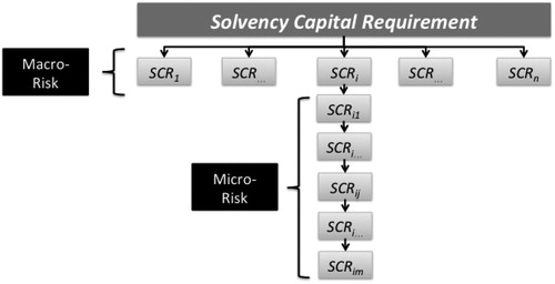
The random variable $L_{ij}^{}$ describes the losses for a one-year time horizon, associated with the j-th micro-risk of the i-th macro-risk. The random variable for unexpected losses is given as, $$Y_{ij}^{}=L_{ij}^{}-E\left(L_{ij}^{}\right)$$

Generic i-th risk depends on the random variable $$Y_{ij}^{}=\sum _j^{m_i}{Y}_{ij}^{}$$

And the total risk of a company will be described by the variable $$Y=\sum _{i=1}^n{Y}_i^{}=\sum _{i=1}^n\sum _j^{m_i}{Y}_{ij}^{}$$

And, therefore, a company’s SCR is defined through the risk measurement of that random variable.

For the ij-th micro risk, the SCR is determined by the unexpected loss at 99.5% of the Value at Risk: $${\mathit{SCR}}_{ij}^{}={\mathit{VaR}}_{99.5\mathrm{\%}}^{}\left(Y_{ij}^{}\right)$$ where for an i-th macro-risk, and as a function of the integrated micro-risks, the SCR is calculated as follows $${\mathit{SCR}}_i^{}=\sqrt{\sum _{x=1}^{m_i^{}}\sum _{y=1}^{m_i^{}}{\mathit{SCR}}_{ix}^{}·{\mathit{SCR}}_{iy}^{}·{\rho }_{ix,iy}^{}}$$ where ${\rho }_{ix,iy}^{}$ represents the linear correlation coefficients proposed by EIOPA.

Eventually, a company’s SCR would turn out: $${\mathit{SCR}}_{}^{}=\sqrt{\sum _{x=1}^{n_{}^{}}\sum _{w=1}^{n_{}^{}}{\mathit{SCR}}_{ix}^{}·{\mathit{SCR}}_{iw}^{}·{\rho }_{ix,iw}^{}}$$ where ${\rho }_{ix,iw}^{}$ represents the linear correlation coefficients proposed by EIOPA.

One of these macro-risks is the market risk that covers one of the most important risks in the insurance sector. Following the same structure, the macro-market risk is composed, in turn, of micro-risks such as interest rate, variable income, real estate and credit quality.

In particular, this work focuses on analysing real estate market risk under the Solvency II regulation with the aim of proposing an internal model to calculate the value at risk or maximum probable loss that an insurer would suffer at the 99.5% confidence level.

2.2. Standard formula for buildings

Property risk represents the risk of loss in the value of property that is owned by an insurer or the adverse change in a property’s market value. To calculate the capital requirement to meet this risk Solvency II through the standard formula proposes to apply a fixed percentage of 25% to the real estate value invested in Europe: $${\mathit{SCR}}_{\mathit{ESTATE}}^{SF}=25\mathrm{\%}·{MV}_{\mathit{ESTATE}}^{}$$ where,

${\mathit{SCR}}_{\mathit{ESTATE}}^{SF}:$Solvency capital required for real estate market risk through the standard formula

${MV}_{\mathit{ESTATE}}^{}:$Market value of the properties.

This 25% was determined based on the Investment Property Databank (IPD) UK Monthly Property Index Total Return, which is only in force in the United Kingdom (Edelstein & Quan, 2006). For that percentage, Solvency II took a historical series of 7 years in the UK market. This is a very liquid market with a very high volatility rate, unlike other countries such as Germany or Spain. The capital thus determined is not very sensitive to risk (Karp, 2007) and it does happen that two companies with different structures in different European countries (and with different risk exposure), can reach the same real estate SCR. This is one of the drawbacks of the standard formula and the alternative to that 25% is to develop an internal model to reduce the capital consumption for real estate investment.

Some authors (Devineu & Loisel, 2009; Pfeifer & Strassburger, 2008) indicate that the standard formula is based on asymmetry and correlation and may not be sufficient for the objectives pursued by Solvency II. Moreover, it rarely adequately reflects the situation to which a company is exposed (Ronkainen et al., 2007). As an alternative, each company can develop its own internal model, although it involves costly and complex procedures (Eling et al., 2007). This model determines the capital that supports the risk, according to each company’s characteristics and the country characteristics and where the properties are located.

These internal models come from the profit testing used since 1980 (Helfenstein et al., 2004; Holzheu, 2000; Liebwein, 2006) were developed because of the need for transparency and supervisory convergence towards solvency and accounting models. On the other hand, they respond to the premise that there is no single common model for all insurance companies that quantifies risk management (Kaliva et al., 2007). Internal models therefore quantify risk to assist in an enterprise’s management and to provide greater returns to shareholders (Berglund et al., 2006; Liebwein, 2006) by usually committing less capital. In addition, there is no need to apply an internal model to a whole company; however, it can be applied to the valuation of certain market risks, such as real estate market risk.

There are few studies on this risk and perhaps the reason for this is due to these assets’ peculiarity, the lack of data from the sector and the lack of normal returns on real estate investments. Real estate is illiquid, has high transaction costs, a high investment value, is heterogeneous and immovable; and the risk of deterioration makes the estimation of its returns and volatilities complicated (Clayton et al., 2008; Geltner et al., 2013). Downs et al. (2016) found that flow analysis of this asset typology is not a good predictor of future returns. In addition, the lack of data causes it to resemble a private equity market, where the market valuation index contains the aggregate sum of the few transactions made. However, the basis for these indices not usually produced daily. At best, it is quarterly or monthly and lacks sufficient historical data to make statistical inference. To determine the 99.5% VaR based on historical data, a minimum of 200 values would be required, asking for a 17-year history on a monthly basis (Amédée-Manesme & Barthélémy, 2018). It is therefore necessary to use other methods to calculate VaR.

3. Real estate market risk modelling

The model initially proposed contemplates the index data to be followed so that past data can be computed. The temporary variations produced (each quarter, month, etc.) provide the variation amount as well as the frequency of variation per invested unit. Therefore, a statistical distribution reflecting the intensity of the change can be obtained, as well as another distribution that reflects the frequency of the change.

The statistical distribution that best reflects the previous frequencies is then determined, using Monte Carlo simulations, to estimate the Value at Risk of a company’s own real estate portfolio.

3.1. The expected loss

Capital at risk will depend both on the frequency of the number of cases where there is a variation in a property’s value and on the intensity of the variation (loss) experienced by a property. So, it is necessary to determine both the frequency function of the claims observed and their severity or intensity (Vegas & Nieto de Alba, 1993). Let´s,

N:The random variable associated with the number of claims occurring in a time interval [0, t) with a probability distribution $P_N(n),$ where n is the realisation of the random variable N.

$X_i$_:Thevariable associated with the amount of the i-th claim that carries an associated probability $V\left(x\right)=P(X_i\le x)$ and x is the realization of the random variable. These variables are independent.

The total amount of claims in that period [0, t), $Y(t)\mathrm{ }$ amounts to $$Y\left(t\right)\mathrm{ }=\mathrm{ }{x}_1\mathrm{ }+\mathrm{ }{x}_2\mathrm{ }+\mathrm{ }\dots +x_{N\left(t\right)}$$

This is, a stochastic process sum of a random number N(t) of independent and equally distributed random variables. The expected loss distribution or total damage in [0, t) is given as $$P\left[Y\left(t\right)\le y\right]=\sum _{n=0}^{\mathrm{\infty }}{P}_N\left(n\right)·V^n\left(y\right)$$

Where,

$P_N\left(t\right):$Probability of n claims in the interval [0, t).

$V^n\left(y\right):$Probability that, having n claims, the sum of the same, reaches the amount y.

The distributions, $P_N\left(t\right)\mathrm{ }$ and${\mathrm{ }V}^n\left(y\right)$ are estimated from observed data.

In this way, the stochastic process number of claims N(t) takes a positive natural number in addition to the null value as there is a possibility that no claims will occur. Likewise, the other random variable, in this case continuous, X, indicates the intensity of the claim, under the hypothesis of an equal distribution of all claims. Therefore, the study of a single variable is sufficient to determine the expected value of a claim.

Once the estimated values have been determined over those observed in the real estate portfolio and for various distribution functions, it is necessary to carry out an analysis of the goodness-of-fit. Therefore, for each distribution function value to be tested, an occurrence probability value similar to those observed must be obtained. This results in the expected portfolio loss for a given degree of plausibility.

3.2. The unexpected loss: VaR

VaR determines the greatest loss for a given probability and for a given period of time. Therefore, an estimate is made in a quartile; and a reasonable estimate needs to be made not only of the distribution mean value but also of the tails. For its definition (Bertrand & Prigent, 2012; Jorion, 2007; Sharpe, 1995) a portfolio C is considered at a time T and a probability p, where a level of losses Y, which must be smaller than or equal to a value, is estimated.

In this way, knowing the distribution of aggregate loss, which are independent and identically distributed, the VaR of losses is defined for $\alpha \mathrm{ }\in \left(0,1\right),$ -${\mathit{VAR}}_{\alpha }(Y(t))$- as, $${P\left({Y\left(t\right))}_{}^{}<{\mathit{VAR}}_{\alpha }\left(Y\right(t\left)\right)\right)=\alpha }_{}$$

This quantile can be estimated by obtaining the distribution function for the period of losses $P[Y(t)\le y].$

The unexpected loss, for practical purposes, involves applying the above-mentioned percentile. This method is widely used in the German market (Altuntas et al., 2011).

Although the concept of VaR is very simple, its calculation can become complex. There is more than one methodology used to calculate it (Abad et al., 2014):

1. Parametric methods. They fit the probability curves to the data and, through statistical inference, obtain the VaR from a given curve. Riskmetrics (Morgan, 1996) is the first model that used the hypothesis of normal distribution and with independent and identically distributed variables (iid).

2. Non-parametric methods. They measure the risk of a portfolio without making assumptions about the variables’ behaviour. They use historical data under the assumption that the nearest future is similar to the recent past and, therefore, past data is used to predict losses in the near future. There are several models that estimate density function from historical simulations (Barone-Adesi et al., 1999; Engle & Manganelli, 2004).

3. Semi-parametric methods. The most significant approaches focus on: Historical Volatility; Filtered Historical Simulation; Quantile Auto-regressions (CaViaR); Extreme Value Theory and Monte Carlo Simulation. Of these, the latter represents perhaps one of the most employed approaches in the insurance sector.

There are works (Deepak & Ramanathan, 2009; Jorion, 2007; Lechner & Ovaert, 2010; Pritsker, 1997; Stambaugh, 1996) that compare the bonanzas by using the historical series, parametric VaR and VaR determined with the Monte Carlo simulation. They generally conclude that there is no one method better than another. On the one hand, parametric methods are simple to implement and very useful when the amount of data is sufficient and the distribution of data follows a normal distribution. On the other hand, the use of Monte Carlo has the great advantage of increasing the number of observations, although it needs a strong computer resource. The direct use of historical data is very accurate for past measures but tends to be poor for future estimates. There is no doubt that each method has its weaknesses and strengths (Stambaugh, 1996), so they should be seen as complementary measures because they provide a greater degree of information according to the circumstances.

The characteristics, as well as the advantages and disadvantages of VaR have been widely discussed in the literature (Artzner et al., 1999; Krokhmal et al., 2011; Pflug, 2000; Rodríguez-Mancilla, 2010), which has measured that an amount over a given horizon and in a given confidence interval will not exceed its losses (Jorion, 2007; Trainar, 2006).

VaR has been methodologically used in Real Estate Investment Trusts (REITs) with the same methodology as that used for bonds and shares. Zhou and Anderson (2012) analysed the loss behaviour of REITs in extreme market conditions, concluding that for different assets, different functions are needed. Liow (2008) uses extreme value theory to assess market risk in ten real estate markets with better results than classic statistics. Jin and Ziobrowski (2011) examines real estate market risk at the portfolio level. It looks at downward market risk in residential housing using conditional volatility models. The analysis carried out finds market differences by region. As an alternative to VaR, real estate market volatility is estimated and predicted using generalized auto-regression conditional heteroscedasticity (GARCH) models with conditional mean, variance and covariance. To support this, the Office Federal Housing Enterprise Oversight (OFHEO) Housing Price Index and the Standard and Poor’s Case-Shiller (S&P/C-S) Index are used as market indices. These indices are available monthly and with data from June 1991 to October 2007. Therefore, there is sufficient data for statistical inference. However, there are no studies on how to apply VaR when there is a lack of data or very little sector data. Even more, VaR jobs in the real estate market are scarce; they usually focus on risk management to give different investment patterns to different investors (Booth et al., 2002). Other authors measure the risk of debt assumed by the purchase of real estate (Gordon & Tse, 2003).

3.3. Parametric VaR

It is also known as VaR calculated through the variance-covariance and delta-normal methods. It is based on the assumption of a normal distribution for the data and its calculation is summarised as a VaR that is proportional to the standard deviation of a portfolio’s performance. Since the portfolio is a linear sum of the data and the data is normally distributed, the portfolio is also normally distributed: $${{\mathit{VAR}}_{\alpha }\left(Y\right(t\left)\right)=\mathrm{Z}\alpha ·{\sigma }_{Y\left(t\right)}}_{}$$

Zα:$\alpha$ percentile of $N(0,1)$

${\sigma }_{S(t)}:$Standard deviation of the portfolio.

This expression has been widely used to calculate the risk values of financial asset portfolios (Deepak & Ramanathan, 2009; Lechner & Ovaert, 2010) where yields on securities follow the normal distribution because they are inappropriate for other asymmetric distributions.

The characteristic that property losses do not follow a normal distribution is a relevant issue for the VaR calculation. Studies (Lizieri & Ward, 2000; Young, 2008; Young et al., 2006) confirm that VaR in buildings is not normal. They would be better described as left-skewed distributions with thick tails (leptokurtosis). Chun et al. (2012) propose to perform regressions by quantiles to estimate the VaR in the last quantiles. They conclude that the VaR of a property portfolio should therefore be calculated using distribution functions with such characteristics or, where appropriate, using industry indices. However, it is generally considered that it is not usual for VaR to follow a normal distribution for high levels of confidence, although this hypothesis of normality is applied by allowing fast and easy computer processing of the data (Amédée-Manesme et al., 2015, 2017).

3.4. Monte Carlo Simulation

The selection of the Monte Carlo method over an analytical approach is made for two reasons (Van Bragt et al., 2010):

1. complexity of the options included.

2. required for solvency reporting and analysis, resulting in more detailed valuations than if less precise analytical approaches were used.

The Monte Carlo method has been used to set parameters in different market price models (Hardy, 2002), such as house prices, as well as interest rates to be used for the valuation of reverse mortgages (Huang et al., 2011; Yang, 2011). It is also used to contrast new paradigms, such as liability-driven investing, through dynamic financial analysis (Van Bragt & Kort, 2011).

Thus, DSII bets on the use of Monte Carlo within an Enterprise Risk Management (ERM) to quantify risks, which even makes it compatible with stress tests (Altuntas et al., 2011).

To know the random loss variable Y(t), it is necessary to set the random variable T on which the previous one depends (Pons & Sarrasí, 2017). This is the index under which the periodic losses of a real estate portfolio are manifested. The w components of this random variable T are also random: $$T=\left(t_1^{},t_2^{},\dots ,t_w^{}\right)$$

T is the random index variable and $t_{\mathrm{i}}^{}$ is the realisation of the same.

Simulation consists of generating a random number, uniformly distributed between 0 and 1, which will correspond to a certain cumulative probability value of this random variable, so that if U is the random number generated in a realisation, then the simulated value of ${\overrightarrow{t}}_i^k$ = s, is: $$\sum _{r=0}^{s-1}P\left(T=r\right)<U\le \sum _{r=0}^{s}P\left(T=r\right)$$

Where ${\overrightarrow{t}}_1^k$ is the performance vector associated with the simulation k-th, with k = 1, 2, …, z of the random variable T and that set of values provide the evolution of the periodic changes of the reference index. Each component ${\overrightarrow{t}}_i^k$ with i = 1, 2, …, w and k = 1, 2, …, z is obtained by Monte Carlo simulation, the random variable T and z is the number of different evolution paths.

Therefore, to obtain by simulation the realisation of ${\overrightarrow{t}}_i^k$ consists of generating a random number, uniformly distributed between 0 and 1. In this way, the probability associated with each performance is always the same, and its value will depend on the number of z simulated trajectories: $$P\left(T={\overrightarrow{t}}_i^k\right)=\frac{1}{z}$$

The number of realisations will depend on the number of simulations. If z is the number of different evolution trajectories, the realisation of the random variable T will be given by the following set of values, $${\overrightarrow{t}}_1^1,{\overrightarrow{t}}_2^2,\dots ,{\overrightarrow{t}}_{\mathrm{i}}^k,\dots ,{\overrightarrow{t}}_{\mathrm{w}}^z$$

Once the distribution function of the random variable T is known, the function random variable distribution of losses Y(t) is obtained, which allows for the confidence level of 99.5% to calculate the VaR of the portfolio.

4. A real estate valuation

4.1. An application to the Spanish real estate market

The internal model will be tested in an insurance company’s real estate portfolio. The objective of this test is to investigate the solvency capital required for this portfolio by applying it against the standard formula. The assumptions on which it is based are as follows:

1. The property investment structure of the insurance company is located in a Spanish town, and its composition does not change over time.

2. the historical database used has been the annual evolution of the Housing Price Index (HPI). This index measures the evolution of the housing prices, both new and second-hand, over time. The data included in the index are acquisitions of dwellings in the reference period within the national territory made by individuals (resident or non-resident in Spain). Purchases and sales made by entities, including financial institutions, are not part of the index. The information source is provided by the General Council of Notaries’ registered dwellings databases, from which the dwellings’ transaction prices, as well as the weightings assigned to each set of dwellings with common characteristics, are obtained (INE, 2018). This data has been obtained from the National Statistics Institute (Appendix A).

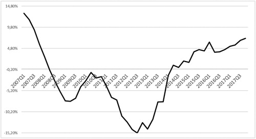
The variation of the index in Spain shows the fluctuations in the housing prices at market value (Appendix A, Table A1), with declines marked by the real estate crisis (Figure 2). From the first quarter of 2014 the variations are positive.

Figure 2. Annual percentage change in the Housing Price Index-HPI-.

Source: National Statistics Institute (INE, 2018).

For a property portfolio with a market value of one million euros, these variations produce a difference in the properties’ value and also generate some negative and positive differences. Therefore, the economic effect of the variation over a four-month period is reflected by the intensity of its loss/gain and the magnitude of quarterly variation in the total of periods contemplated, depending on the frequency in the period under study.

From the historical data, the observed and accumulated frequencies (Figures 3 and 4) and the classic statistics are obtained (Appendix B, Table B1). Specifically, the average variation in the price of the property portfolio per quarter amounts to €15,522, with a standard deviation of €73,951. That is, a low average but with a great dispersion. On a portfolio valued at one million euros, the extreme values of maximum decrease and maximum quarterly increase would be €152,000 of maximum decrease; and the greatest quarterly increase would be €131,000.

Figure 3. Theoretical frequencies.

Source: Own work.

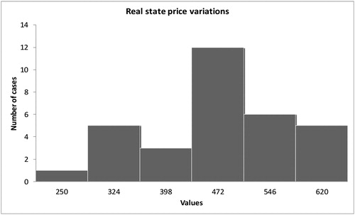
Figure 4. Theoretical frequencies.

Source: Own work.

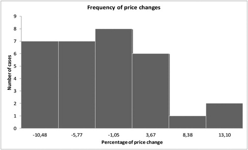
4.2. The statistics function

The observed frequency is sourced from historical data and is contrasted with the individual theoretical frequencies of various functions to observe which function most faithfully reflects reality (Appendix B, Tables B3 and B4). Adjustment to a series of distributions using the maximum likelihood technique and testing the goodness-of-fit through various tests such as Kolmogorov-Smirnov, Chi-square and Anderson-Darling, has been done with code developed in Visual Basic™, and with the spreadsheet Excel™. As for the severity or intensity of the loss, Figures 5 and 6 indicate which functions are closest to the observed frequencies. Normal, log-normal and gamma distribution are highlighted.

Figure 5. Theoretical and practical frequencies Variation of the HPI.

Source: Own work.

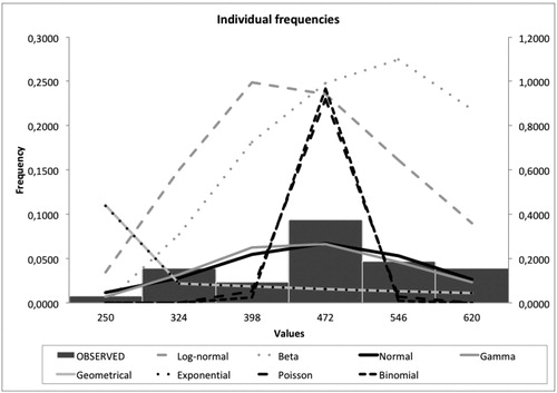
Figure 6. Cumulative theoretical and practical frequencies variation of the HPI.

Source: Own work.

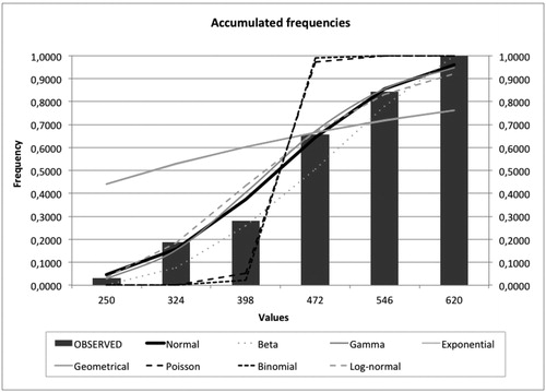
After carrying out the distribution goodness-of-fit test (Kolmogorov–Smirnov, Chi-square and Anderson–Darling tests, whose values are reflected in Appendix B – Tables B5–B7), it is found that the function that best replicates the frequency of the number of claims in this case is the Normal one (Table 1).

Table 1. Ranking of distributions.

Kolmogorov–Smirnov		Chi-2		Anderson–Darling
0,0939	Normal	5	Normal	0,4714	Normal
0,1225	Gamma	6	Gamma	0,4777	Log-normal
0,1518	Log-normal	7	Log-normal	0,5064	Gamma
0,1494	Beta	10	Beta	1,5405	Beta
0,4080	Exponential	77	Exponential	2,2582	Exponential
0,3162	Poisson	77	Geometric	2,2780	Geometric
0,3345	Binomial	48.836.071	Poisson	7,9921	Poisson
0,4097	Geometric	62.593.385.224	Binomial	12,8741	Binomial

Source: Own work.

The distribution function that best represents the real estate prices’ evolution in Spain is the Normal one. Therefore, the required solvency capital is calculated based on the standard formula, parametric VaR and the VaR with the Monte Carlo method.

4.3. Results and discussion

With regard to the standard formula, a value at risk is obtained with a confidence interval of 99.5% during a financial year of $${\mathit{SCR}}_{\mathit{ESTATE}}^{SF}=\mathrm{€}250,000$$

This value is obtained by applying a 25% shock to the properties’ market value.

With respect to parametric VaR, the value at risk is calculated as follows $${\mathit{SCR}}_{\mathit{ESTATE}}^{\mathit{PVaR}}=\mathrm{Z}\alpha ·{\sigma }_{Y\left(t\right)}^{}$$ where

$Z\alpha =F_x^{-1}\left(0.995\right)=2.576$, where F is the distribution of the cumulative function of a normal random variable and ${\sigma }_{Y(t)}^{}$ is the variation in the value of real estate. It turns out, therefore: $${\mathit{SCR}}_{\mathit{ESTATE}}^{\mathit{PVaR}}=\mathrm{ }\mathrm{€}190,498.06$$

This is a significantly lower capital requirement. However, although it is a simple method to implement and the distribution follows a normal distribution, the amount of data is insufficient to ensure statistical robustness. Therefore, it is evaluated through Monte Carlo to save the data sufficiency.

The Monte Carlo simulation used 10,000 different scenarios generated with the distribution obtained through the Excel™ spreadsheet functions. The obtained value of the real estate portfolio with a confidence interval of 99.5% during a fiscal year after the simulation of those scenarios, amounts to €800,400.07. So, the unexpected loss or value at risk of the real estate investment would be: $${\mathit{SCR}}_{\mathit{ESTATE}}^{IM}=\mathrm{€}199,599.93$$

A value lower than the standard formula is somewhat higher than the parametric VaR because it contemplates 10,000 different scenarios (Figure 7), however, does contemplate statistical inference, while the former suffered from a number of values sufficient to be statistically significant.

Figure 7. Frequency distribution and VaR of the property portfolio.

Source: Own work.

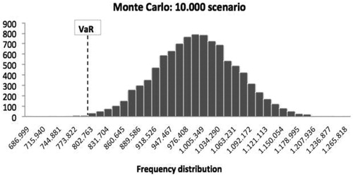
In relative terms, this implies that the consumption of capital by means of an internal model would be 19.96% as opposed to the 25% established by the standard formula.

Through the application of stochastic simulation, it is possible to

• determine a specific procedure to provide an internal model that determines the capital required for solvency in the case of real estate market risk, without making an assumption about a certain distribution function for historical data. In any case, the VaR of a real estate portfolio must be calculated using distribution functions resulting from source data analysis. However, Solvency II is committed to using VaR in general to calculate the capital required for most risks

• obtain probabilistic results, unlike deterministic analysis. In this way, through stochastic simulation, the results show not only what can happen but also how likely a result will be.

• estimate the total amount of claims for every one of the possible scenarios (according to a certain confidence interval) since the stochastic simulations consist of thousands of possible claims scenarios. Furthermore, by considering, as well as quantifying, the amount of the historical data of the claims, it is possible to calculate the probability of every projected scenario.

• know the influence that a specific part of the investment portfolio has, due to its special characteristics (industrial sector buildings, services, geographical location, etc.). In this way, it is possible to calculate the unexpected loss according to the simulation proposed for that portfolio and quantify the influence it has on the final economic capital of the company. In other words, it assesses the increased risk effect posed by a specific part of the portfolio.

• use it as a tool for company management to incorporate temporary variation in parameters, thick tails and extreme scenarios; and, therefore, it can cover a wide range of risks

• apply this internal model for the specific case of Spain. The internal model developed has shown that capital consumption for real estate market risk is less than the 25% established in Solvency II, which allows insurers to have less capital at risk.

As limitation of the work, the literature says that property losses do not follow a normal distribution, however when studying the distribution in Spain, Normal distribution fits the best. It may possibly be due to not having enough data and history in Spain to know if is this is a characteristic of Spanish property market, or the period chosen, or the scarce number of observations of the Housing Price Index. In any case, if the property losses do not follow a normal distribution, expected shortfall should be used, as Basel III, Basel IV regulations and Swiss solvency test propose.

5. Conclusion

The importance of solvency in the insurance sector has become a fundamental issue in last years. Recent regulatory has focused in risk valuation in order to assess soundness of insurance companies and at the same time calculate solvency capital requirements according to the real risk assumed by the firms.

This paper contributes to the literature presenting an internal model to value real state risk in insurance firms. The aim of this work has been to establish a procedure to provide an internal model that values real estate market risk and calculates the capital that guarantees it. This enables the loss distribution function to be incorporated into the valuation model.

The fact that the real estate market has suffered major crises means that conventional risk measures are not entirely valid and the literature has been delved into to measure it through VaR. As a response to the standard formula, the proposed internal model will also be set in a housing price index, but will generate scenarios in a way that allows statistical inference. This may be useful for regulators and companies.

A further development of the model may be to segment the information of the employed HPI index according to the geographical location of the dwellings within Spain in order to particularize the consumption of capital by real estate investment, as well as choosing a data period in which there is no economic crisis. This would make it possible to check whether, in a period without different fluctuations, the variation in real estate price follows a normal distribution or not.

Acknowledgments

This work was supported by Consolidated Research Group Eusko Jaurlaritza/Gobierno Vasco EJ/GV: IT 897-16. The authors acknowledge language help from Julie Walker-Jones.

Disclosure statement

No potential conflict of interest was reported by the authors.

Appendix A.

Historical sample of the Housing Price Index in Spain

 

Table A1. Annual percentage change in the Housing Price Index.

Year / Quarter.	Q1	Q2	Q3	Q4
2017	5,3	5,6	6,7	7,2
2016	6,3	3,9	4	4,5
2015	1,5	4	4,5	4,2
2014	−1,6	0,8	0,3	1,8
2013	−14,3	−12	−7,9	−7,8
2012	−12,6	−14,4	−15,2	−12,8
2011	−4,1	−6,8	−7,4	−11,2
2010	−2,9	−0,9	−2,2	−1,9
2009	−7,6	−7,7	−7	−4,3
2008	2,8	−0,3	−3	−5,4
2007	13,1	11,6	9,2	5,7

Source: National Statistics Institute (INE, 2018).

Appendix B.

Statistics and goodness-of-fit

From historical data, the classic statistics (mean, variance, etc.) are obtained from the variations experienced by the housing price index.

The data is adjusted to a series of distributions using the maximum likelihood technique and testing the goodness-of-fit through various tests such as Kolmogorov–Smirnov, Chi-square and Anderson–Darling.

Each data series is adjusted to a series of distributions (Table B2) depending on the data characteristics with respect to distributions. Goodness-of-fit is analysed, such that $$p=\left.\mathit{max}\right|F_n^{}\left(x\right)-\left.F\left(x\right)\right|$$ where F_n corresponds to the values of the empirical and adjusted distributions, respectively.

Table B1. HPI statistics.

Average	Typical Deviation	Variance	α-Gamma
−1.552273	7.395111	54.687669	0.044060
β- Gamma	Log-normal Media	Typical Log-normal Dev.	λ-Exponential
−35.230709	1.515018	0.944659	−0.644217

Source: Own work.

Table B2. Common distributions in the insurance sector.

Discrete	Continuous
Binomial Poisson Binomial Negative	Gamma Beta Pearson Log-gamma Normal Log-normal

Source: Own work.

Table B3. HPI variation statistics.

Average	Typical deviation	α-Gamma	β-Gamma	Media log-normal
−1.552273	7.395111	47.215223	73.951.111644	1.515018
Min	−15.200000	α-Beta	α-Gamma	Typical deviation Log-normal
Max	13.100000	1.309944	0.000033	0.944659
Difference between legs	5	Average-Beta	β-Gamma	λ-Exponential
No. of sections	6	0.416272	−47.640.540444	−0.644217
Interannual variation	Frequency accumulated	Frequency Individual	Frequency acumulated (%)	Frequency
−10.48	7	7	0.225806	0.225806
−5.77	14	7	0.451613	0.225806
−1.05	22	8	0.709677	0.258065
3.67	28	6	0.903226	0.193548
8.38	29	1	0.935484	0.032258
13.10	31	2	1.000000	0.064516

Source: Own work.

Calculation of the individual and cumulative theoretical frequencies of the variation of the housing price index.

Table B4. Theoretical frequencies of the HPI variation.

Individual frequencies (%)
Observed	Normal	Gamma	Log-normal	Beta	Exponential	Poisson	Binomial	Geometric
0.0313	0.0449	0.0266	0.0344	0.0000	0.4392	0.0000	0.0000	0.4409
0.1563	0.1120	0.1269	0.1499	0.0770	0.0882	0.0000	0.0000	0.0881
0.0938	0.2182	0.2503	0.2487	0.1818	0.0744	0.0511	0.0234	0.0742
0.3750	0.2695	0.2671	0.2358	0.2480	0.0627	0.9213	0.9674	0.0625
0.1875	0.2108	0.1846	0.1610	0.2746	0.0528	0.0276	0.0092	0.0527
0.1563	0.1045	0.0925	0.0901	0.2185	0.0445	0.0000	0.0000	0.0444
Cumulative Frequencies (%)
Observed	Normal	Gamma	Log-normal	Beta	Exponential	Poisson	Binomial	Geometric
0.0313	0.0449	0.0266	0.0344	0.000000	0.4392	0.0000	0.0000	0.4409
0.1875	0.1569	0.1535	0.1843	0.077017	0.5275	0.0000	0.0000	0.5290
0.2813	0.3751	0.4038	0.4331	0.258805	0.6018	0.0511	0.0234	0.6032
0.6563	0.6446	0.6708	0.6689	0.506852	0.6645	0.9724	0.9908	0.6657
0.8438	0.8554	0.8555	0.8299	0.781453	0.7173	1.0000	1.0000	0.7184
1.0000	0.9598	0.9480	0.9200	1.000000	0.7618	1.0000	1.0000	0.7627

Source: Own work.

Table B5. Goodness-of-fit of the HPI variation. Test Kolmogorov–Smirnov.

Kolmogorov–Smirnov
		Normal	Gamma	Log-normal	Beta	Exponential	Poisson	Binomial	Geometric
		0.094	0.123	0.152	0.149	0.408	0.316	0.335	0.410
Level 0.1%.	0.220	Ok	Ok	Ok	Ok	x	x	x	x
Level 0.05%.	0.240	Ok	Ok	Ok	Ok	x	x	x	x
Level 0.01%.	0.288	Ok	Ok	Ok	Ok	x	x	x	x

Source: Own work.

Table B6. Goodness-of-fit of the HPI variation. Test Chi-2.

Chi-2
		Normal	Gamma	Log-normal	Beta	Exponential	Poisson	Binomial	Geometric
		4.690	6.176	7.414	9.968	76.981	48.836.070	62.593.385.223	77.281
Level 0.1%.	7.78	Ok	Ok	Ok	x	x	x	x	x
Level 0.05%.	9.49	Ok	Ok	Ok	x	x	x	x	x
Level 0.01%.	13.28	Ok	Ok	Ok	Ok	x	x	x	x

Source: Own work.

Table B7. Goodness-of-fit of the HPI variation. Anderson test–Darling.

Anderson–Darling
		Normal	Gamma	Log-normal	Beta	Exponential	Poisson	Binomial	Geometric
		0.471	0.506	0.478	1.541	2.258	7.992	12.874	2.278
Level 0.1%.	1.929	Ok	Ok	Ok	Ok	x	x	x	x
Level 0.05%.	2.502	Ok	Ok	Ok	Ok	Ok	x	x	x
Level 0.01%.	3.907	Ok	Ok	Ok	Ok	Ok	x	x	x

Source: Own work.

References

- Abad, P., Benito, S., & López, C. (2014). A comprehensive review of value at risk methodologies. The Spanish Review of Financial Economics, 12(1), 15–32. doi:10.1016/j.srfe.2013.06.001
- Altuntas, M., Berry-Stölzle, T. R., & Hoyt, R. E. (2011). Implementation of enterprise risk management: Evidence from the German property-liability insurance industry. The Geneva Papers on Risk and Insurance - Issues and Practice, 36(3), 414–439. doi:10.1057/gpp.2011.11
- Amédée-Manesme, C.-O., Barthélémy, F., & Keenan, D. (2015). Cornish Fisher expansion for commercial real estate value at risk. The Journal of Real Estate Finance and Economics, 50(4), 439–464. doi:10.1007/s11146-014-9476-x
- Amédée-Manesme, C.-O., Barthélémy, F., Prigent, J.-L., Keenan, D., Mokrane, M. (2017). Modified Sharpe ratios in real estate performance measurement: Beyond the standard cornish fisher expansion. THEMA Working Paper 20. Université de Cergy-Pontoise.
- Amédée-Manesme, C.-O., & Barthélémy, F. (2018). Ex-ante real estate value at risk calculation method. Annals of Operations Research, 262(2), 257–285. doi:10.1007/s10479-015-2046-7
- Artzner, P., Delbaen, J., Eber, M., & Heath, D. (1999). Coherent measures of risk. Mathematical Finance, 9(3), 203–228. doi:10.1111/1467-9965.00068
- Barone-Adesi, G., Giannopoulos, K., & Vosper, L. (1999). VaR without correlations for nonlinear portfolios. Journal of Futures Markets, 19(5), 583–602. doi:10.1002/(SICI)1096-9934(199908)19:5<583::AID-FUT5>3.0.CO;2-S
- Berglund, R., Koskinen, L., & Ronkainen, V. (2006). Aspects on calculating the Solvency capital requirement with the use of internal models. 28th International Congress of Actuaries. http://www.ica2006.com/Papiers/3001/3001.pdf
- Bertrand, P., & Prigent, J.-L. (2012). Gestion de portefeuille: Analyse quantitative et gestion structurée. Économica.
- Booth, P., Matysiak, G., & Ormerod, P. (2002). Risk measurement and management for real estate portfolios. (Tech. Rep.). IPF.
- Braun, A., Schmeiser, H., & Siegel, C. (2014). The impact of private equity on a life insurer’s capital charges under solvency II and the Swiss solvency test. Journal of Risk and Insurance, 81(1), 113–158. doi:10.1111/j.1539-6975.2012.01500.x
- Byrne, P. J., & Lee, S. (2001). Risk reduction and real estate portfolio size. Managerial and Decision Economics, 22(7), 369–379. doi:10.1002/mde.1026
- Callender, M., Devaney, S., Sheahan, A., & Key, T. (2007). Risk reduction and diversification in UK commercial property portfolios. Journal of Property Research, 24(4), 355–375. doi:10.1080/09599910801916279
- Chun, S. Y., Shapiro, A., & Uryasev, S. (2012). Conditional value-at-risk and average value-at-risk: Estimation and asymptotics. Operations Research, 60(4), 739–756. doi:10.1287/opre.1120.1072
- Clayton, J., MacKinnon, G., & Peng, L. (2008). Time variation of liquidity in the private real estate market: An empirical investigation. Journal of Real Estate Research, 30(2), 125–160.
- Cuoco, D., & Liu, H. (2006). An analysis of VaR-based capital requirements. Journal of Financial Intermediation, 15(3), 362–394. doi:10.1016/j.jfi.2005.07.001
- Deepak, J., & Ramanathan, T. (2009). Parametric and nonparametric estimation of value at risk. The Journal of Risk Model Validation, 3(1), 51–71. doi:10.21314/JRMV.2009.034
- Devineu, L., & Loisel, S. (2009). Risk aggregation in Solvency II: How to converge the approaches of the internal models and those of the standard formula? Bulletin Français d’Actuariat, 9(18), 107–145.
- Downs, D. H., Sebastian, S., Weistroffer, C., & Woltering, R.-O. (2016). Real estate fund flows and the flow-performance relationship. The Journal of Real Estate Finance and Economics, 52(4), 347–382. doi:10.1007/s11146-015-9539-7
- European Commission (EC). (2003). Solvency II – Reflections on the general outline of a framework directive and mandates for further technical work. Note to the IC Solvency Subcommittee MARKT/2539/03.
- Edelstein, R., & Quan, D. (2006). How does appraisal smoothing bias real estate returns measurement? The Journal of Real Estate Finance and Economics, 32(1), 41–60. doi:10.1007/s11146-005-5177-9
- European Insurance and Occupational Pensions Authority (EIOPA). (2012). Technical specifications for the solvency II valuation and solvency capital requirements calculations (Part I). https://eiopa.europa.eu.
- Eling, M., & Holzmueller, I. (2008). An overview and comparison of risk-based capital standards. Journal of Insurance Regulation, 26(4), 31–60.
- Eling, M., Schmeiser, H., & Schmit, J. T. (2007). The solvency II process: Overview and critical analysis. Risk Management & Insurance Review, 10(1), 69–85. doi:10.1111/j.1540-6296.2007.00106.x
- Engle, R. F., & Manganelli, S. (2004). CAViaR: Conditional autoregressive value at risk by regression quantiles. Journal of Business & Economic Statistics, 22(4), 367–381. doi:10.1198/073500104000000370
- Fitch Ratings. (2011). Solvency II set to reshape asset allocation and capital markets. Insurance Rating Group Special Report.
- Garayeta, A., & De La Peña, J. I. (2017). Looking for a global standard of solvency in the insurance industry: Pros and cons of three systems. Transformations in Business and Economics, 16(41), 55–74.
- Garayeta, A., Iturricastillo, I., & De La Peña, J. I. (2012). Evolución del capital de solvencia requerido en las aseguradoras españolas hasta solvencia II. Anales del Instituto de Actuarios Españoles, 18, 111–150.
- Geltner, D., Miller, N., Clayton, J., & Eichholtz, P. (2013). Commercial real estate analysis and investments. 3rd ed. Cengage Learning, Inc.
- Gordon, J. N., & Tse, E. W. K. (2003). VaR: a tool to measure leverage risk. The Journal of Portfolio Management, 29(5), 62–65. doi:10.3905/jpm.2003.319907
- Granito, I., & De Angelis, P. (2015). Capital allocation and risk appetite under Solvency II framework. Cornell University Library. doi:10.13140/RG.2.1.1136.8404
- Hardy, M. R. (2002). Bayesian risk management for equity-linked insurance. Scandinavian Actuarial Journal, 2002(3), 185–211. doi:10.1080/034612302320179863
- Helfenstein, R., Scotti, V., & Brahin, P. (2004). The impact of IFRS on the insurance industry. Swiss Re Sigma, 7, 1–34.
- Hernández, R., & Martínez, M. I. (2012). Capital assessment of operational risk for the solvency of health insurance companies. Journal of Operational Risk, 7, 43–65.
- Holzheu, T. (2000). Solvency of non-life insurers: Balancing security and profitability expectations. Swiss Re Sigma, 1, 1–38.
- Huang, H. C., Wang, C. W., & Miao, Y. C. (2011). Securitisation of crossover risk in reverse mortgages. The Geneva Papers on Risk and Insurance - Issues and Practice, 36(4), 622–647. doi:10.1057/gpp.2011.23
- Instituto Nacional de Estadística (INE). (2018). Índice de Precio de la Vivienda. https://www.ine.es/consul/serie.do?s=HPI948
- Jin, C., & Ziobrowski, A. J. (2011). Using value-at-risk to estimate downside residential market risk. Journal of Real Estate Research, 33(3), 389–413.
- Jorion, P. (2007). Value at risk: The new benchmark for managing financial risk. McGraw-Hill.
- Kaliva, K., Koskinen, L., Ronkainen, V. (2007). Internal models and arbitrage – free calibration. AFIR colloquium. http://www.actuaries.org/AFIR/Colloquia/Stockholm/Kaliva.pdf
- Karp, T. (2007). International solvency requirements – Towards more risk-based regimes. The Geneva Papers on Risk and Insurance - Issues and Practice, 32(3), 364–381. doi:10.1057/palgrave.gpp.2510139
- Krokhmal, P., Zabarankin, M., & Uryasev, S. (2011). Modeling and optimization of risk. Surveys in Operations Research and Management Science, 16(2), 49–66. doi:10.1016/j.sorms.2010.08.001
- Lechner, A., & Ovaert, T. (2010). Techniques to account for leptokurtosis and asymmetric behaviour in returns distributions. The Journal of Risk Finance, 11(5), 464–480. doi:10.1108/15265941011092059
- Liebwein, P. (2006). Risk models for capital adequacy: Applications in the context of solvency II and beyond. The Geneva Papers on Risk and Insurance - Issues and Practice, 31(3), 528–550. doi:10.1057/palgrave.gpp
- Liow, K. H. (2008). Extreme returns and value at risk in international securitized real estate markets. Journal of Property Investment and Finance, 26(5), 418–446.
- Lizieri, C., Ward, C. (2000). Commercial real estate return distributions: A review of literature and empirical evidence. Working Paper 2000-01.
- Morgan, J. P. (1996). Riskmetrics technical document. J. P. Morgan.
- Pfeifer, D., & Strassburger, D. (2008). Solvency II: Stability problems with the SCR aggregation formula. Scandinavian Actuarial Journal, 2008(1), 61–77. doi:10.1080/03461230701766825
- Pflug, G. C. (2000). Some remarks on the value-at-risk and the conditional value-at-risk. In S. Uryasev (Ed.), Probabilistic constrained optimization: Methodology and applications. Springer.
- Pons, M. A., & Sarrasí, F. J. (2017). Simulación de Monte Carlo aplicada a un modelo interno para calcular el riesgo de mortalidad en Solvencia II. Recta, 18, 53–70.
- Pritsker, M. (1997). Evaluating value-at-risk methodologies: Accuracy versus computational time. Journal of Financial Services Research, 12(2/3), 201–242. doi:10.1023/A:1007978820465
- Rodríguez-Mancilla, J. R. (2010). Living on the edge: How risky is it to operate at the limit of the tolerated risk?. Annals of Operations Research, 177(1), 21–45. doi:10.1007/s10479-009-0604-6
- Ronkainen, V., Koskinen, L., & Berglund, R. (2007). Topical modelling issues in Solvency II. Scandinavian Actuarial Journal, 2, 135–146.
- Sharpe, W. (1995). Forework. En R. Beckstrom and A. Campbell. An introduction to the Var. Palo Alto, CA: CATS software, pp. i–iii
- Solvency II. (2009). Directiva del Parlamento Europeo y del consejo, de 25 de noviembre de 2009, sobre el seguro de vida, el acceso a la actividad de seguro y de reaseguro y su ejercicio (Solvencia II). 2009/138/CE. (2009).
- Stambaugh, F. (1996). Risk and value at risk. European Management Journal, 14(6), 612–621. doi:10.1016/S0263-2373(96)00057-6
- Trainar, P. (2006). The challenge of solvency reform for European insurers. The Geneva Papers on Risk and Insurance - Issues and Practice, 31(1), 169–185. doi:10.1057/palgrave.gpp
- Van Bragt, D., Steehouwer, H., & Waalwijk, B. (2010). Market consistent ALM for life insurers—Steps toward solvency II. The Geneva Papers on Risk and Insurance - Issues and Practice, 35(1), 92–109. doi:10.1057/gpp.2009.34
- Van Bragt, D., & Kort, D. J. (2011). Liability-driven investing for life insurers. The Geneva Papers on Risk and Insurance - Issues and Practice, 36(1), 30–49. doi:10.1057/gpp.2010.36
- Vegas, J., & Nieto de Alba, U. (1993). Matemática Actuarial. Ed. Mapfre.
- Yang, S. S. (2011). Securitisation and tranching longevity and house price risk for reverse mortgage products. The Geneva Papers on Risk and Insurance - Issues and Practice, 36(4), 648–674. doi:10.1057/gpp.2011.26
- Young, M., Lee, S., & Devaney, S. (2006). Non-normal real estate return distributions by property type in the UK. Journal of Property Research, 23(2), 109–133. doi:10.1080/09599910600800302
- Young, M. (2008). Revisiting non-normal real estate return distributions by property type in the U.S. The Journal of Real Estate Finance and Economics, 36(2), 233–248. doi:10.1007/s11146-007-9048-4
- Zhou, J., & Anderson, R. (2012). Extreme risk measures for international REIT markets. The Journal of Real Estate Finance and Economics, 45(1), 152–170. doi:10.1007/s11146-010-9252-5