Business intelligence appraisal based on customer behaviour profile by using hobby based opinion mining in India: a case study

Abstract

This research study contributes towards understanding the customer’s behaviour dynamics. In business analysis, it is very important not to ignore the fact that the interaction between human beings implicitly includes an emotional dimension. The research methodology includes the following: (1) customer purchase pattern prediction methods based on correlation; (2) augmentation of data set by using genetic algorithms; and (3) multiple regression models. The analysis indicates how the hobby of a customer is directly related to the purchase patterns and satisfaction level. We applied business intelligence (BI) techniques and concluded that, by using multiple regression method is possible to evaluate the level of customer satisfaction up to the upper limit of security of about 90%. BI tools could be used to employ significant achievements in specific fields based on open innovations. This paper aims at providing further practical guidance in this innovative research field by using a mix of interdisciplinary methods and techniques.

Keywords:

• Customer business intelligence
• consumer behaviour
• multiple regression opinion analysis
• hobby
• genetic algorithm
• economic sustainability

SUBJECT CLASSIFICATION CODES:

• C10
• D11
• M21

1. Introduction

The core idea of business intelligence (BI) is to recognise the behavior of the customer and to predict their purchase pattern for improvement of the business as well as for a better environmental sustainability. Efficient decision making based on BI is essential to ensure competitiveness for sustainable growth (Jin & Kim, 2018). However, in literature, there is no universally accepted definition of BI. BI plays an essential role in areas such as sales representatives’ performance, customer loyalty, and product performance (Athanasoulias & Chountalas, 2019). Remarkable BI applications have also been reported in a wide variety of occupational fields, from health care and airlines to major IT and telecommunication firms (Watson, 2009). Cebotarean (2011) suggested that BI is related to computer-based techniques used in spotting, digging-out, and analyzing business data, such as sales revenue by products and/or departments, or by associated costs and incomes. Larson and Chang (2016) argued that BI includes an information value chain for gathering raw data, turning these data into useful information, management decision making, driving business results, and raising corporate value.

Amberg and Fogarassy (2019) suggested that knowledge can influence the entire decision-making process of consumers. Martin et al. (2012) argued that BI can be applied to absolutely all decision making and prediction analysis. Most of the customers either use or donate or through away products which they feel unwanted, but causing economic expenditure for both national economies and global economy. Hence consumer behavior observance should help avoid non-usage of purchased products for a sustainable buying behavior and to avoid binge practices. Hence, this work focuses on how the hobbies of a person influence his/her purchase of a product to the real world purchase pattern. Our research study also analyses the opinion of the customer on the purchased product. Since, the type of data required depends purely on behavioral aspects of the respondents, further proceedings of data collection was done by collecting the live data from the people of different professions, age groups, genders etc.

The remainder of our research study is organised as follows: The first section includes the introduction, and other relevant dimensions of the research topic. This research paper tries to use genetic algorithm (GA) and multiple correlations for the empirical analysis, which is distributed as follows: Section 2 presents a complex literature review, Section 3 introduces the research methodology and mathematical preliminaries, Section 4 debates and critically evaluates the results and analysis framework and Section 5 highlights the final conclusions including limitations and future research directions.

2. Literature review

The changes in consumer behaviour had strong influences on all enterprises throughout time. A decision moment occurred in the 1970s when a significant macroeconomic change affected the law of supply and demand. Currently, customers face diverse offers which leads customers’ decision process to be more complicated and their behavior become unpredictable. Until 1960, the economic perspective of consumer behaviour and the models relied on the assumption that all consumers were always rational in their purchases. Consequently, consumers will always purchase the product which brings their higher satisfaction. Before 1979, scientists developed three different models, i.e. the economic model, the learning model, and finally the psychoanalytic and sociological model (Le & Liaw, 2017). The ‘hungry shopper’ example illustrates a proposition that has been systematically explored in numerous studies: forecasts of future hedonic and emotional states are anchored in the current emotional and motivational state. The outcome has been labeled a ‘projection bias’ (Loewenstein et al., 2003) since consumers are seemingly projecting their current mental state onto a future one (Kahneman & Thaler, 2006). Steinley (2006) conducted a survey on k-means algorithm. k-means is a simple version of finite mixture of model and several methods are developed by using this procedure may have some degree of transferability to other modeling methods. Many data reduction methods are analysed.

The research work of Makarenkov and Legendre (2001) is based on the weighted correlation coefficient between the decision making credentials and other parameters of the customer. A statistical tool such as correlation is used to determine the degree to which two variables are related. It also examined the relation between two independent variables of a given set of data containing information about a product and personal. Weights are given on the basis of this coefficient and frequency analysis of the credentials. Using these weights, the patterns of maximum weights are formed as a cluster. Modha and Spangler (2003) proposed an idea to integrate numerous feature spaces. Such research paper uses the k-means clustering methodology, which will minimise the dispersion inside the cluster and maximise it in between the clusters along with all the feature spaces. Compared to the simple term ‘matching’, the procedure of weighting gave them considerable. Huh and Lim (2009) highlighted the aim of weighted k-means clustering method. They argued that a naive scheme may lead to unstable degenerate variable weights and optimisation criterion with the penalty term yields more stable and reasonable solutions. This is illustrated with three well-known standardised forms of Olive oil data to yield better clustering structures than the ordinary k-means clustering in the sense of counting the number of misclassified observations. The algorithm successfully classifies the observations perfectly.

Zhang et al. (2019) adopted the same objective function used by Huh and Lim (2009) and proposed a more suitable optimisation method. This method can significantly improve the original method in terms of both algorithm stability and clustering accuracy, especially on high-dimensional datasets. Deng et al. (2010) proposed a clustering approach based on a new mathematical model in each iteration the algorithm fixes cluster centers and used some conditions to obtain the optimal clusters memberships. They proved that the mentioned conditions are sufficient and important for optimality of clusters memberships when cluster centers are fixed. Xu et al. (2013) worked on W-k-means which is an automated two-level variable weighting clustering algorithm for MultiView data. His procedure significantly performed well. Makarenkov and Legendre (2001) preferred to use optimal variable weighting rather than k-means clustering, while using Monte Carlo simulation. They experimented on a huge set of data using variable weighting algorithms in comparison with additive tree reconstruction and k-means partitioning.

On the other hand, Nguefack-Tsague (2014) revealed that difficult optimal model averaging schemes fail to exist under square error loss if it comes to different estimators. The authors proved it by deriving the optimal weighting scheme and demonstrated that these weights are not optimal when the parameters are estimated. Huang et al. (2005) focused on a new k-means algorithm using current groups, which helps calculate variable weights automatically with the help of clustering process, iterative procedure and variance of the distances inside of the cluster. Deng et al. (2014) came up with an idea to assigns weights to terms so that it can improve the working of sentiment analysis and other text mining scenarios. Here, seven statistical functions are used to understand the importance of a term for expressing sentiments for every term from the learning files with each category.

In a previous research study, BI was perceived as a concept used by almost every chief financial officer, controller, and analyst in order to make to make more intelligent business decisions (Rasmussen et al., 2002). Moreover, behavioural BI focuses on the people and their behaviours, the environment and various constraints that influence their behaviours (Shrivastava & Lanjewar, 2011). Essential pillars such as management buy-in, the availability of BI reports and the provision of reporting guidelines are positively interconnected with effective strategic planning (Calitz et al., 2018). The personalised, individualised, and relevant information of the customers are required for BI appraisal.

This study mainly focuses on behavioural data analysis of the customers based on emotional factor. This emotional factor typically is considered as hobby (Pilon, 2016). It is important to reveal how emotional factor influences consumer behaviour. The typical dataset contains customer’s hobbies, gender, occupation, age group, annual income, product category, opinion on the product purchased etc. These credentials are used to predict the customer purchase pattern. Moreover, companies achieve a high degree of efficiency by avoiding multiple transportation modes.

GAs are algorithms that simulate the logic of Darwinian natural selection theory considering that the most suitable attributes are selected from a set of attributes. Classification accuracy can be improved by reducing the number of attributes. Nevertheless, data mining is a broad term with multidimensional implications. Vijayarani and Sudha (2013) argued that data mining is ready for application in the business community because it is supported by three technologies that are now sufficiently mature: Massive data collection, Powerful multiprocessor computers and data mining algorithms.

Sharma (2013) used GA based on software test data generator to test cases andexamined if GAs are adaptable to different environments. GAs have power in adapting to different environment. The study also revealed that GAs are suitable in searching the input domain for the required test sets. Mehboob et al. (2014) provided a detailed survey of applications of GA using different kinds of GA techniques. Many procedures have been worked on and compared with the efficiency of suggested GA to random testing technique and roulette wheel method. Velasco et al. (2017) proposed a classification system for selection and data augmentation algorithm which generates synthetic glucose time series from real data. Their results showed that, in a scarce data context, the grammatical evolution models can get more clear and robust predicts using scenario selection and data augmentation. Muller and Freytag (2015) used a few attributes to find the existence of heart disease using the GA technique. The methodology helps in diagnosing heart issues which reduces the number of test for a patient.

3. Research methodology

Building strong customer relationship is essential for businesses. Companies are interested in meeting their customer needs, but also to obtain useful informations from them which can be used for innovation. Consequently, a higher degree of sales productivity and reliability can be achieved. Technically, the aim of this research is to identify customer purchase pattern based on the information they provide to the business.

When a customer purchases a product, is important to understand that various factors affect the decision making capacity of the customer in each situation. The action taken by an individual usually reflects his psychosomatic characteristics. According to a new survey (Pilon, 2016) conducted by AYTM market research, the results are the following:

• 74% of overall respondents consider having hobbies to be important

• 66% said that they wish they had more time for hobbies in their lives

• 29% of respondents said that they frequently make purchases related to their hobbies

• 51% says they only make sometimes hobby related purchases

• 16% said they rarely do

• 4% never do

The hobby of a person is an innermost desire which they pursue by trying to fulfil their unmet needs. A silent person may choose to have solitary hobbies like photography, reading, cooking etc. Social people tend to have hobbies that are more people-oriented like adventurous sports. A homemaker can develop hobbies like cooking, gardening, shopping etc. These choices can reinforce themselves. The next section deals with the design of the system which relates customer’s information based on hobby field for purchase prediction.

This research study covers the related area of customers behavioural credentials such as: hobby, occupation, age group etc. We will refer to both attribute and parameter as ‘field’ (Nethravathi & Karibasappa, 2016, 2017a, 2017b). The set of attributes/credentials of a customer is referred as a ‘data record’ instead of the word record in general. Moreover, the words field, attribute and parameter are used with the meaning of ‘gene’ instead of field or attribute and the set of genes are referred as ‘chromosome’ instead of data record. The collection of chromosome is referred as ‘chromosomes’ since it is related to GA. The methodology contains three main parts, i.e.:

1. Method of prediction of the customer purchase pattern based on correlation;

2. Augmentation of data set by GAs;

3. Multiple regression models.

These applied methods are explained in the following subsections.

3.1. Prediction of the customer purchase pattern based on a correlation

Correlation technique is used to calculate weights of the data record fields. By using these weights, customers are clustered based on their hobbies. Out of the data collected manually, clusters including different hobbies are formed. For example, a cluster contains customers with the adventurous sports, another cluster with the hobby cooking, one more cluster with the hobby reading etc. These clusters are used to predict the new customer who visits to a web page first time to buy a product. Based on the behavioural attributes of the new customer, he/she will be assigned to a particular cluster. The model predicts and recommends what the customer is looking for before he purchases the products. Correlation technique is used to find the relationship between two fields. The value obtained for the field is so-called weight. Based on the value of the field, we can consider how much they are interrelated or connected. Highly related fields are clustered and are used for prediction. It is realised from the literature review performed on the topic of clustering that the previous research work used k-means algorithm and distance measure formulas to make the clusters. It is realised that correlation technique gives more relation to the data items. According to the definition of correlation, highly correlated records gives positive relation and less correlated records gives negative correlation. Weighted correlation method is used to cluster the dataset. These weights measure the significance of the field and indicate their contribution, while tracking consumer buying behaviour. Similar or equal weighted data stuffs are gathered together based on logical relationship. We need to assign weights to all the fields of the data record. In this study, the ‘hobby’ field is used and kept aside and then we found the relation between hobby field and age group, hobby and occupation, hobby and income group etc. This procedure is explained below:

Let the total data in the whole dataset be n and the rejected after first filtering, data is R; the remaining data set D_s is shown in equation (1)(1) $$D_s=\left(n-R\right)$$(1) (1) $$D_s=\left(n-R\right)$$(1)

Here, the rejected data are shown as percent in equation (2)(2) $$R=\frac{D_s}{n}\times 100$$(2) : (2) $$R=\frac{D_s}{n}\times 100$$(2)

The data in$\mathrm{ }{D}_s\mathrm{ }$ is considered for the next step called evaluation of correlations coefficient. Let this$\mathrm{ }{D}_s\mathrm{ }$ be written as $y_{\text{ij}}.$ Let a single dataset be: (3) $$D_s=y_{\text{ij}}=x_{\text{ij}},y_{i1k},y_{i2k}{y}_{i3k}\mathrm{\dots }{y}_{\text{imk}}$$(3) where i indicates the i^th value of the dataset which runs from 1,2…n and m is the number of attributes to be correlated with reference to the value $x_{\text{ik}}{x}_{ik}$ in which, k is the third dimension of the data attribute which varies from 2 to k. Let us consider for each $x_{\text{ik}}{x}_{ik}\mathrm{ }$ total of n number of such datasets. For these n numbers of the dataset using the following equation (4)(4) $$r_{xy}=\frac{{\sum }_{l=1}^n{x}_{lk}{y}_{il}\frac{{\sum }_{l=1}^n{x}_{ik}{\sum }_{l=1}^n{y}_{il}}{n}}{\sqrt{\left({\sum }_{l=1}^n{x}_{ik}^2-\frac{{\left({\sum }_{l=1}^n{x}_k\right)}^2}{n}\right)·}}\mathrm{ }$$(4) , the correlation coefficients are calculated. (4) $$r_{xy}=\frac{{\sum }_{l=1}^n{x}_{lk}{y}_{il}\frac{{\sum }_{l=1}^n{x}_{ik}{\sum }_{l=1}^n{y}_{il}}{n}}{\sqrt{\left({\sum }_{l=1}^n{x}_{ik}^2-\frac{{\left({\sum }_{l=1}^n{x}_k\right)}^2}{n}\right)·}}\mathrm{ }$$(4) Where, $r_{\text{xy}}$ represents, correlation coefficient with respect to x_ik, considering all y’s till n number of the dataset. Coming to the dataset we have parameter considering ‘adventurous sports’ as a hobby as x₁ first we calculated the correlation between the hobby to other credentials that is y_i’s, like occupation, gender, age group, income group, main product category, sub category, satisfaction level, advocacy level. This correlation coefficient is the reference relation between x_i’s and y_i’s, but these y_i’s contain k subcategories/classes in them.

It is necessary to map the correlation coefficient for all these k sub categories of y_i’s. This is done by analyzing the data on the basis of frequency of occurrence of k sub categories, and distributing the correlation coefficient accordingly as follows.

Lets consider a category y_ij includes k sub categories as shown in the equation (3)(3) $$D_s=y_{\text{ij}}=x_{\text{ij}},y_{i1k},y_{i2k}{y}_{i3k}\mathrm{\dots }{y}_{\text{imk}}$$(3) . Frequency of occurrence of each entity of this y_ijk sub-sample will be f₁, f₂, f₃, … f_k, so that it satisfies the condition given in equation (5)(5) $${\sum }_{i=1}^k{f}_i=N\mathrm{ }$$(5) , N: the total number of dataset concern to the area of interest. (5) $${\sum }_{i=1}^k{f}_i=N\mathrm{ }$$(5)

The distribution of correlation or weight of each sub categories can be calculated with respect to $r_{{\text{xy}}_k}$ is refereed as in equation (6), so that the equation (7)(7) $$r_{\text{xy}}=\sum r_{\text{xyi}\mathrm{ }}$$(7) satisfies the equation (6). This equation (7)(7) $$r_{\text{xy}}=\sum r_{\text{xyi}\mathrm{ }}$$(7) is also considered $r_{{xy}_k}=\frac{\left(r_{xy}\times f_k\right)\mathrm{ }}{N}\mathrm{ }$(6) as weights of the respective data of y_i’s. (7) $$r_{\text{xy}}=\sum r_{\text{xyi}\mathrm{ }}$$(7)

This $r_{\text{xy}}{r}_{xy}$ is also considered as $w_{\text{xy}}{w}_{xy}$ where w is considered as weights similarly: (8) $$w_{{xy}_k}={\left(\frac{w_{xy}\times f_k}{n}\right)}_{}{w}_{\text{xy}}=\left(\frac{w_{\text{xy}}\times f_k}{N}\right)w_{{xy}_k}={\left(\frac{w_{xy}\times f_k}{N}\right)}_{}\mathrm{ }$$(8)

After evaluating the frequency based weights from the equation (8)(8) $$w_{{xy}_k}={\left(\frac{w_{xy}\times f_k}{n}\right)}_{}{w}_{\text{xy}}=\left(\frac{w_{\text{xy}}\times f_k}{N}\right)w_{{xy}_k}={\left(\frac{w_{xy}\times f_k}{N}\right)}_{}\mathrm{ }$$(8) for each x_ik’s, or for each hobby’s, with respect to each entity and also its sub-sample y_ijk’s, shows the readiness for the next process.

In this process, each dataset is evaluated as the abridge of each weights, which is the weights of the correlation between x_i’s and y_i’s, of the dataset by summing up the weights of each y_ijk’s, as per the equation (9)(9) $$w_{\text{dsj}}={\sum }_{j=1}^m{w}_{\text{xyjk}}{\mathrm{ }w}_{{ds}_j}={\sum }_{j=1}^m{w}_{{xy}_{jk}}$$(9) : (9) $$w_{\text{dsj}}={\sum }_{j=1}^m{w}_{\text{xyjk}}{\mathrm{ }w}_{{ds}_j}={\sum }_{j=1}^m{w}_{{xy}_{jk}}$$(9)

Where $w_{\text{dsj}}$ indicates the total weight for the single data string or one dataset.

Next step is to cluster the whole dataset as per maximum weights of the data string of each (hobby) category. In this work it is considered as top 10% of the maximum total weights of single datasets are clustered together.

The correlation coefficient r_xy between a hobby ‘adventurous sports’ and the rest of the attributes can be observed here. Table 5 gives the value of correlation index by applying the equation (1)(1) $$D_s=\left(n-R\right)$$(1) for all the attributes with the hobby ‘adventurous sports’.

Similarly, this procedure is applied to the rest of the hobbies.

The next stage of the process is to split the aggregate correlations as per the counts or frequency of occurrences of each data as per equation (9)(9) $$w_{\text{dsj}}={\sum }_{j=1}^m{w}_{\text{xyjk}}{\mathrm{ }w}_{{ds}_j}={\sum }_{j=1}^m{w}_{{xy}_{jk}}$$(9) . For example, split hobby ‘reading’ to age group correlation as per number of k values of equation (6) proportionately. For example, say, after calculating the correlation values for all the hobbies, 0.2868% correlation is obtained for the hobby ‘reading’ to age group field. This is calculated as follows by using the equation (7)(7) $$r_{\text{xy}}=\sum r_{\text{xyi}\mathrm{ }}$$(7) .

As the manual data collection is difficult and also consumes more time, GA technique is applied to the datasets, which are collected manually.

3.2. Enhancement of the customer dataset using a GA

It is inferred from the result obtained based on correlation analysis that it is possible to achieve accurate results with more number of the dataset, which is applied on behavioural analysis of the customer. As the manual data collection was tedious, it is decided to enhance the data by using GA procedure. The practical data was collected from people working in various public and private sectors such as City Corporation, Mangalore Refinery and Petrochemical Ltd., Engineering Colleges, Kakunje Software Pvt. Ltd., Accolade software solutions, Bharath Mall, Giriyas, KSRTC bus stand, Railway Station etc. The data was also collected by sending the questionnaires by using google form. The graduate engineering students and post graduate students were pursuing degrees in education at Shree Devi Institute of Technology, Mangalorein India. The google forms were posted to the students’ parents in various regions like Mumbai, Gujarath, Madhya Pradesh and other places of Karnataka in order to achieve the uniformity and consistency in databases. Figure 1 explains the steps and illustrates the methodology of dataset augmentation.

Figure 1. Block schematic of the data augmentation process.

Source: Author’s computation.

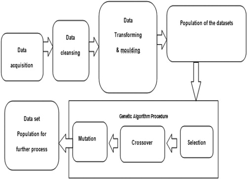
Previous literature used dataset which was not available to us, suck as Amazon and other online websites. Our research is concentrated on behavioural analysis, which requires customer hobby, profession, customer satisfaction on the product. We encountered difficulties in gathering already available data, which is required for this work. This work is not a company initiated project. The available online dataset does not contain this behavioural information. Hence it was decided to collect the data by communicating with the people from different age group, different profession etc. The data collected from the government and private organisation of Indian sub-continent is being referred to as live data/manual data collection. Correlation technique was not used in any of the previous research papers we studied. Correlation technique have not been applied for customer dataset in the previous works. We realised that JAVA language is appropriate and easy for coding, while is used along with the statistical software. Figure 1 illustrates the process of generating a dataset using a GA.

3.2.1. Flow of a typical GA

The correlation coefficient method presented above, efficiently builds the clusters of the customers. The grouping of data set is based on its correlation value which descends from highest value to lowest. Table 5 summarises the correlation weights obtained between a hobby Adventurous sports to the rest of the fields of the dataset belong to the same hobby. Table 6 explained how the weights are distributed for a sample data record. The grouping of data set is based on its correlation value which descends from the highest value to lowest (or in other words, from the maximum value to minimum value). The results obtained from this part is explained in section 4.2. This shows that the purchase behaviour of a person is related to hobby to the real-world purchase pattern. It is inferred from this result that, the accuracy of the output can be increased with the more number of dataset.

Literature survey is performed to augment the dataset. As our work related to behaviour of human beings, it is realised that GA is best suited for the enhancement of the behavioural dataset, which was collected by communicating with people directly. These dataset have been multiplied by using GA techniques. GAs are a sort of computational model and offer a viable solution to a certain problem on a simple chromosome-like data-structure. Evolution process occurs on chromosomes based on rules of selection, crossover and mutation. The crossover mechanism resembles to natural biological reproduction. At this step, more than one parent is chosen and one or more child is produced by using the genes of the parents. To obtain a new solution, mutation uses a random tweak in the chromosome. It is used to preserve and introduce variety in the genetic populace. Generally crossover is applied with high probability and mutation is applied with a low probability.

As a first step, the existing chromosomes (referred to as a dataset in the previous section) are randomly populated. Out of these n chromosomes, a chromosome (referred as a data record in the previous section) R1 is selected and all the genes (referred as field or attributes previously) of R1 that is p0, p1…pt will be copied to the new chromosome Rng1. The gene set Rng1, is taken for further process of crossover and mutation. In this Rng1 one or a few genes (Pi, Pj…Pl) are selected, for crossover and mutation. Gene Rng1 is represented in Figure 2 (one field represented in 8 bits) and similarly Gene Rng2 is depicted in this Figure 3 in order to demonstrate the crossover operation. The crossover process of a single gene (field) is explained with the help of Figures 2 and 3.

Figure 2. Bit patterns of p_i^th gene of Rng1.

Source: Author’s computation.

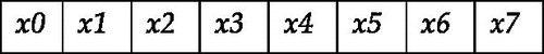
Figure 3. Bit patterns of p_i^th gene of Rng2.

Source: Author’s computation.

Crossover: In this study, the crossover process uses a random operation to generate a new chromosome from two parent chromosomes. As explained in the previous section after copying the chromosome into a new chromosome Rng1, one more chromosome R2 is selected from the set of n chromosomes and taken for crossover. Since it is preferable to carry out the crossover for the chromosomes, randomly from the new chromosome set some chromosomes p_i have been selected for the process of crossover. These selected bits from the gene (p_i’s) of Rng1 are replaced from those of R2 gene.

The chromosomes undergo evolution process based on selection, mutation and crossover. Each individual receives a fitness value in the environment and the highest values are selected for reproduction. The crossover procedure swaps two data (called as gene) in two chromosomes. Example: From a chromosome, which is having genes p0, p1…pt. one gene is selected. Similarly, the same type of gene is selected from another chromosome. Let for example one gene of p_iis selected randomly that contains the bits labelled as x in our example showed in Table 1 below. Similarly, the same type of the gene is selected from R2 and labelled as a new gene just like it is described in Table 1. To understand the crossover operations of genes, an example is considered and is depicted in Table1. We have represented a gene in 8 bits long and performed the crossover operation in the example.

Table 1. Values of the two sample genes – x and y.

x	0	1	1	0	0	1	0	1
y	1	1	0	0	0	1	1	0

Source: Author’s computation.

Example: The following Table 1 reveales an example depicting the values written for two sample genes x and y.

Copy the second random gene, which is y to a new gene (i.e. off spring). This randomly selected gene2 (y) is described in the following Table 2 such as:

Table 2. Values of the gene y.

New gene

1

1

0

0

0

1

1

0

Source: Author’s computation.

We replaced the value of new gene by using x’s bits, i.e. select 3 genes (it is bits) from the x and changed the corresponding genes bits in the new gene i.e. y. The following Table 3 illustrates this operation below.

Table 3. Replacing the value of the bits in new gene using x – values.

								
x	0	1	1	0	0	1	0	1
New gene	1	1	0	0	0	1	1	0

Source: Author’s computation.

After replacing three bits in the new gene, the values are shown in Table 4 below.

Table 4. Value of the new gene after the crossover operation.

New gene

1

1

1

0

0

1

0

1

Source: Author’s computation.

According to chromosome, maximum value of gene is still 8 binary bits, so that crossover will happen randomly for any of these 8 bits. It may be 3 bits, 4 bits, 5 bits or all 8 bits changes may happen. The new offspring is generated by crossover operation.

Mutation: The above crossover gene shown in Table 4 is further taken for the mutation. The process of mutation is as shown in Figure 4. In this process of mutation, the most significant bit is written as it is as Y0. 0^th bit and first bit are XORed the resultant is placed in the first bit of the resultant gene that is resultant of Y0⊕X1. XOR operation is a logical operation that outputs true only when its inputs differ. First and second bits are XORed to get the result as a second bit, that is, X1⊕Y2 leads to the resultant of the third bit. Similarly, all the bits are calculated as shown in Figure 4, for the process of mutation. The advantage of this method is there is no overflow and data loss also it lies within the limits since MSB is not changed.

Figure 4. Example showing method of mutation for a given gene.

Source: Author’s computation.

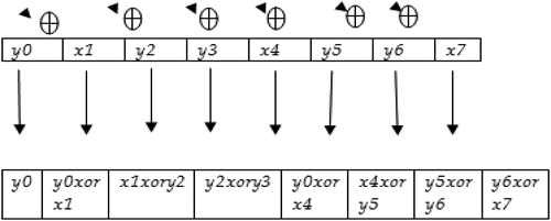
Example for mutation: This will be demonstrated as the new gene after mutation of 11100101 is illustrated next. To maintain the trace earlier gene, x1 will be written as it is in the new gene. x1 is XORed with x2 written in the position of x2. x2 is XORed with x3 written in the position of x3. Similarly, it will continue till the end that is x8. The new gene generated in this example is 10010111. After this process of mutation, the resultant gene is introduced in the chromosomes and the chromosome is tested for the validation. The next section explains the process of validation.

3.2.2. Validation rules for the enhanced dataset

To ensure the resultant chromosome is in line with the existing chromosome, which is nearer to the real life and correctness of the chromosomes is validate during the association rule. This validation procedure is applied to the enhanced dataset. The resultant data record is rejected in case if it satisfies the association rules. Few rules mentioned below:

1. Gender = male and occupation = Home maker

2. Age group = below 19 and occupation other than the student

3. Satisfaction level = Extremely dissatisfied and advocacy level = Likely/Most Likely

Using data augmentation, the dataset is enhanced. The dataset generated by using GA’s are validated and considered for processing in the next stage. It is observed from the result of correlation analysis that, the value between satisfaction levels and advocacy level in product purchase can be improved. Next stage proposes the usage of multiple regression technique to create a stronger cluster of customer using enhanced dataset using a GA.

3.3. Multiple regression models to get more appropriate results

The relationship between two variables can be predicted, by taking the ratio of the covariance between them. To find a single variable from the weighted linear sum of numerous variables, multiple regressions can be applied. Using linear function on a set of different variables, the coefficient of multiple correlations on a given variable can be predicted.

In many situations, more than one regressor or variable is applicable in regression analysis, which is called multiple regression models. In many situations, more than one regressor or variable is applicable in regression analysis, which is called multiple regression models. Since each parameter contributes for the output, each parameter is multiplied by an appropriate weight which is evaluated by regression analysis. This work uses eight parameters as shown in Table 6, we have related them to tally the equation. If there is variation in one parameter, this variation impact on results. To rectify this impact, we are evaluating based on regression analysis. This work used matrix method of multiple regression and is explained below.

Table 5. The output of correlations between ‘Adventures Sports’ and the rest of credentials.

S. No.	Credentials	Correlation value
1	Gender	97.1536%
2	Occupation	87.5816%
3	Age group	93.7938%
4	Annual income	93.3520%
5	Product category	80.1001%
6	Sub category	74.7264%
7	Satisfaction level	94.2809%
8	Advocacy level	97.3041%
9	Happiness	75.4851%

Source: Author’s computation.

Table 6. Weights of the single sample data record.

Name of the attribute	Category	Weighted correlation for concern category
Gender	Male	0.0194
Occupation	Engineer	0.0330
Annual income	Below Rs. 2.5 L	0.0196
Age group	20-29 yrs	0.0160
Product category	Clothing	0.0211
Sub category	Men	0.0125
Satisfaction level	Extremely satisfied	0.0230
Advocacy level	Likely	0.0415

Source: Author’s computation.

The set of D_s is considered for evaluation of the coefficient of correlations. Let a single dataset be equation (3)(3) $$D_s=y_{\text{ij}}=x_{\text{ij}},y_{i1k},y_{i2k}{y}_{i3k}\mathrm{\dots }{y}_{\text{imk}}$$(3) as said earlier. The dependent variable is one that has to be predicted. Variables used to predict the value of the dependent variable are called regressor variables.

In equation (9)(9) $$w_{\text{dsj}}={\sum }_{j=1}^m{w}_{\text{xyjk}}{\mathrm{ }w}_{{ds}_j}={\sum }_{j=1}^m{w}_{{xy}_{jk}}$$(9) $x_{\mathit{imk}}\mathrm{ }$ is dependent variable, which is evaluated, basedon the following independent variables (10) $$x_{i1},y_{i2k},y_{i3k},y_{i4k}\dots y_{i\left(m-1\right)k}$$(10)

In multiple regression, the value of $x_{\mathit{imk}}$ is evaluated from the following equation (11)(11) $$x_{\mathit{imk}}={\overrightarrow{\beta }}_0+{\overrightarrow{\beta }}_1\times y_{i2k}+{\overrightarrow{\beta }}_2\times y_{i3k}+{\overrightarrow{\beta }}_3\times y_{i4k}+\dots +{\overrightarrow{\beta }}_{m-1}\times y_{i\left(m-1\right)k}+\epsilon \mathrm{ }$$(11) : (11) $$x_{\mathit{imk}}={\overrightarrow{\beta }}_0+{\overrightarrow{\beta }}_1\times y_{i2k}+{\overrightarrow{\beta }}_2\times y_{i3k}+{\overrightarrow{\beta }}_3\times y_{i4k}+\dots +{\overrightarrow{\beta }}_{m-1}\times y_{i\left(m-1\right)k}+\epsilon \mathrm{ }$$(11)

Where: $\epsilon ,$ error component; coefficients ${\overrightarrow{\beta }}_0,{\overrightarrow{\beta }}_1,{\overrightarrow{\beta }}_2,{\overrightarrow{\beta }}_3\dots {\overrightarrow{\beta }}_{\left(m-1\right)}$ are regression weights; $\overrightarrow{{\beta }_0}\mathrm{ },$ y intercept; $\overrightarrow{{\beta }_1}\mathrm{ }$ determines the contribution of the independent variable indicating that it is coefficient of independent variable $y_{i2k};$ $\overrightarrow{{\beta }_j}\mathrm{ }$ used to find $y_{\mathit{ijk}}.$ Weights are calculated as follows:

We used dataset $\overrightarrow{D_{s_i}} =y_{i2k},y_{i3k},y_{i4k}\dots y_{i\left(m\right)k}$ i from 1: n as a matrix${\overrightarrow{\mathrm{ }D}}_{s\mathrm{ }}$ has m columns and n rows. Value of $x_{\mathit{imk}}$ is the independent variable and this is calculated on the base of other dependent variables $x_{i1},y_{i2k},y_{i3k},y_{i4k}\dots y_{i\left(m-1\right)k}$ i from 1 to n.

In equation (13)(13) $$\left[\beta \right]={\left\{\left[{D_{s_{}}}^T\right]\times \left[D_{s_{}}\right]\right\}}^{-1}\times \left\{\right[{D_{s_{}}}^T]\times [y_{\mathit{imk}}]\mathrm{ }$$(13) we use the following: (12) $$y_m=\overrightarrow{D_s}\overrightarrow{\beta }+\epsilon$$(12)

The regression weights$\overrightarrow{\mathrm{ }\beta }\mathrm{ }$ is obtained by equation (13)(13) $$\left[\beta \right]={\left\{\left[{D_{s_{}}}^T\right]\times \left[D_{s_{}}\right]\right\}}^{-1}\times \left\{\right[{D_{s_{}}}^T]\times [y_{\mathit{imk}}]\mathrm{ }$$(13) : (13) $$\left[\beta \right]={\left\{\left[{D_{s_{}}}^T\right]\times \left[D_{s_{}}\right]\right\}}^{-1}\times \left\{\right[{D_{s_{}}}^T]\times [y_{\mathit{imk}}]\mathrm{ }$$(13)

After evaluating$\mathrm{ }\beta \mathrm{ }$ matrix, the value of independent variable $x_{\mathit{imk}}$ can be calculated for every record. We obtain the weights for individual fields at this stage and$\overrightarrow{\mathrm{ }\beta \mathrm{ }}$ is having the total weight of all the fields of a data record. This procedure is applied for the dataset which was collected manually and for the enhanced dataset also. The value for the satisfaction field obtained for manual data and enhanced dataset is compared for ten hobbies. The result is explained in Table 7, it shows that results are accurate after applying multiple regression for the enhanced dataset. This is explained in section 4.2.

Table 7. Evaluation of TPR values for 10 hobbies.

S. No.	1	2	3	4	5	6	7	8	9	10
Hobby	1	2	3	4	5	6	7	8	9	10
TPROR*	91.3	86.6	86.1	83.7	89.4	94.1	95.6	96.6	98.1	96.5
TPRER**	83.33	90.6	97.1	94.10	92.95	91.07	89.23	90.2	84.26	87.83

TPROR, True Positive Ratio of satisfaction level for the original records; TPRER, True Positive Ratio of satisfaction level for enhanced records.

According to regression formula in equation (13)(13) $$\left[\beta \right]={\left\{\left[{D_{s_{}}}^T\right]\times \left[D_{s_{}}\right]\right\}}^{-1}\times \left\{\right[{D_{s_{}}}^T]\times [y_{\mathit{imk}}]\mathrm{ }$$(13) , we need to add an error at the time of finding relations to a data record. The difference between $x_{\mathit{imk}}\mathrm{ }\mathit{and}\mathrm{ }\widehat{x_{\mathit{imk}}}\mathrm{ }$ can be represented as epsilon, which gives error component. This is represented a$\epsilon$ in this work. Further, it is observed that if we optimise the error value of $\epsilon ,$ it still possible to obtain the quality of the clusters in better way. Hence this work attempted to reduce the error value. The error reduction process is explained below.

New value of $x_{\mathit{imk}}$ is evaluated andthe average errorvalue is also calculated based on the error obtained by all the value of $x_{\mathit{imk}}\mathrm{ }$ is based on existing dataset. This process is repeated until error is optimised. Equation (13)(13) $$\left[\beta \right]={\left\{\left[{D_{s_{}}}^T\right]\times \left[D_{s_{}}\right]\right\}}^{-1}\times \left\{\right[{D_{s_{}}}^T]\times [y_{\mathit{imk}}]\mathrm{ }$$(13) uses this error value for assessing new data record $x_{\mathit{imk}}.$ Usage of equation (11)(11) $$x_{\mathit{imk}}={\overrightarrow{\beta }}_0+{\overrightarrow{\beta }}_1\times y_{i2k}+{\overrightarrow{\beta }}_2\times y_{i3k}+{\overrightarrow{\beta }}_3\times y_{i4k}+\dots +{\overrightarrow{\beta }}_{m-1}\times y_{i\left(m-1\right)k}+\epsilon \mathrm{ }$$(11) helps in predicting values for new independent data record on the basis of an existing dataset.

4. Empirical analysis and results

After defining the methodology, it is intended to use in the data collected for the analysis. As per the equation (2)(2) $$R=\frac{D_s}{n}\times 100$$(2) after cleansing, the rate of data rejection from the original data is 0.6 percentages. These data are taken for the next step that is to find the relation between the attributes of the dataset with respect to the intended attribute ‘hobby’.

There are two experiments for which we are analyzing and interpreting the results, as follows:

•Evaluation using correlation analysis

•Evaluation using a multiple regression model, these are shown in the next section.

4.1. Evaluation using correlation analysis

Table 5 below shows the results after evaluation of correlation coefficient for all the 9 fields of the dataset. The next step is the distribution this weight obtained for a specific field will be distributed to its sub categories. This is calculated with respect to $r_{{\text{xy}}_k}$ as refereed in equation (7)(7) $$r_{\text{xy}}=\sum r_{\text{xyi}\mathrm{ }}$$(7) .

For example, according to the results obtained in Table 5, consider hobby to gender correlation $r_{\text{xy}}$= 0.9715. Distribute this correlation weights to its sub categories i.e. to male and female. There are 60% of male records and 40% of female records in the dataset. That is 0.9715 0.6 = 0.5829 is the weight for the male and for female 0.9715 0.4 = 0.3886. The same procedure is used to find the weights for the subcategories of other fields. Then, these weights will be assigned to data records based on their sub-categories. For example, after splitting weights for the subcategories, one of the data records shows the value for different categories as shown in Table 6.

The summing up of all entities in Table 5 for all the dataset is evaluated and top 10% of the total data record for a particular hobby is clustered together. The new data record is tested on the basis of thisdataset. Next, some of the observations on the dataset have been elaborated.

Among many observations found from the outcome of this stage, we mention the following:

1. The age group between ‘20–29 yrs’. One can observe 39% of people purchased ‘electronics’ products like ‘laptop, mobile phones, TV’s’ etc. and few of them purchased ‘clothing’. By this one can conclude that there may be a strong correlation between the hobbies to the gender.

2. Age group between ‘20–29 yrs’ customers purchased ‘electronics’ products, 17.2% of customers purchases ‘mobile phones’, 1.9% of customers purchased ‘TVs’, 2.6% of customers purchased ‘laptop’ and 1.9% purchased ‘camera’, rest 7.9% of customers are not purchased anything. We can say that the majority of teachers between ‘20–29 yrs’ age group purchases ‘mobile phones’. This shows that the behavioural attributes of a customer is directly related to their purchase of a product.

By using a GA, the existing customer dataset is enhanced. From the dataset, randomly two data records are picked to generate a new (child) record. The hobby parameters of these two records along with age group, occupation, income group and satisfaction are crossed over correspondingly to get the new chromosome. Random 3, 4, 5, 6, and 7 bits are used for crossing over of genes.

The newly generated gene is further mutated to modify its characteristics as per the GA procedure. This new gene is vetted through methods to check whether suits for real world scenario. For example, a chromosome with age group ‘below 19 yrs’ with a high-income group is considered invalid. Similarly records with conflicting values for satisfaction level and advocacy level, e.g. one data record having value ‘very dissatisfied’ with the product and ‘most likely’ advocating it to others. In this part of the research study, the dataset is increased by three times of the original dataset.

4.2. Evaluation using multiple regression model

Customer credentials used to judge how satisfied a customer is for the product they have purchased. Using the above information, this work measures the satisfaction level of the consumer. Table 7 below depicts the results of satisfaction level, which tallies with the existing data with a high percentage. Figure 5 showing a variation of 83.7 to 98.1 of true + vevalue in predicting satisfaction level for the manually collected dataset. It ensures that TPR value is not less than 83.7. Real True Positive RatioTPR values for satisfaction level for ten hobbies after data enhancement are depicted in Figure 6 presented below.

Figure 5. The variation in values when considering 10 hobbies.

Source: Author’s computation.

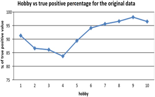
Figure 6. The variation in values with the enhanced dataset for 10 hobbies.

Source: Author’s computation.

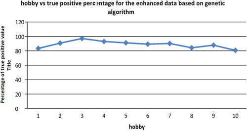
The average TPR crosses 91.8% for 10 hobbies.

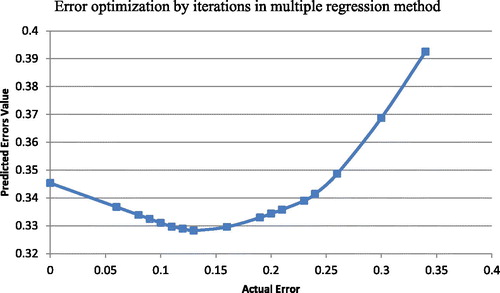
Likewise, other attributes are considered for evaluating TPR, coefficient calculated based on multiple regression as given in equation (12)(12) $$y_m=\overrightarrow{D_s}\overrightarrow{\beta }+\epsilon$$(12) , the estimation of the credential is done, based on the assumption that error ε = 0. Observed from the result that it is possible to predict the customer behaviour better, if the error values are at its minimum. This is done after checking the estimated value of the data record with the original value. Now the average error is evaluated based on the existing record by evaluating the error for all the data set. Further calculation is done on the basis of average error and this process will be repeated. Beginning of the process the error starts decreasing and it reaches a minimum point after which it starts increasing. The values of the iterations are shown in Figure 7 and the error is evaluated and plotted in the graph. This indicates the error estimated in this method will come to a minimum point at 0.16 values. Still, further reduction of the error is not possible. This is suitably used in the work to evaluate the customer purchase pattern based on one of the credentials.

Figure 7. Evaluation of min. error by several iterations in multiple regression.

Source: Author’s computation.

After applying multiple regressions to the enhanced data set the more accurate value of satisfaction to an accuracy level is achieved i.e. between89 to 90%. Better results are obtained from the multipleregression over a single correlation. The results will be better when the quantity of the dataset is increased by using GAs and rule of association. 30% of the data set is increased by applying GA to the original set. Table 7 shows the outcome of the enhanced dataset.

5. Conclusions

Initially, the data records are clustered on the basis of weights using correlation technique, which is explained in the section 3.1. It is observed from the result and analysis that, with the huge data records, it is still possible to improve the accuracy of the result. As the data collection through communicating with the people is tedious and time consuming, it is decided to enhance the data using GA and is demonstrated in the section 3.2. The techniques of GA are applied with different bits of crossover operations and mutation. The newly generated data record is further mutated to modify its characteristics as per the GA procedure. GAs provide a well-established framework for implementing artificial intelligence tasks such as classification, learning, and optimisation. The results revealed that out of total records, 0.6 percentages are rejected due to improper data and also due to manual filtering. After applying weighted correlation methodology for dataset in the first part of this work, some of the results found shown below:

• A housewife with hobby ‘cooking’ tends to purchase the household item and she is satisfied with that product and her advocacy level is between 80% and 89%,

• Also, housewife with hobby ‘cooking’ purchases an electronic category product and her satisfaction level is comparatively good and advocacy level is between 89% and 90%.

• Considering a record with the hobby ‘adventurous sports’ and he purchases sports accessories and he is in almost all cases satisfied and his advocacy level is between 89% and 90%.

This is an indication of BI. For example, among the dataset we have, the customers with the hobby ‘cooking’ and they have purchased household items, electronic products. On the other hand, we have the customers with the hobby ‘adventurous sports’ and they have purchased sports accessories. This experiment proves our theory of relating hobby of a person to the real world purchase pattern. When a customer visits a business place for the first time, the products he/she is looking for may be recommended based on the customer behavioural attributes. This makes this work different from the existing one. Unlike the existing online businesses displays products based on previous purchases. At the Data enhancement stage, two records are randomly selected from the existing dataset for the creation of new data record. Multiple attribute crossovers and mutation procedure generated a good combination for the generation of the new record. Using this technique, a large number of the dataset are multiplied. By using multiple regression, more focused results are obtained. It is seen that multiple correlations gives more accurate results compared to a single correlation. As there is increase in the volume of the dataset it is possible to predict the more accurate result, which is listed in Table 6. There is around a 30% increase in the volume of the dataset from original which is demonstrated in the analysis.

It is concluded that, by using the multiple regression method is possible to evaluate the value of the satisfaction level to the advocacy level of an average 89 to 90%. This is important because if a customer is satisfied with the purchased product, then he must recommend the same product to others as well. This is the third contribution of our work. The outcome of the multiple regressions is worked again for the reduction and optimisation of the error. The fourth contribution of this work is to optimise the error value of the field happiness. Based on the value of the happiness field, this work predicts whether the customer is happy with the purchased product or not. By applying multiple regression method for the enhanced dataset, value of the happiness field is predicted. Figure 7 depicts that the error value obtained is 0.344 at the beginning. This is reduced to 0.16 by multiple iteration method. The prediction percentage is increased with this method. This indicates that, it is possible to predict the purchase behaviour of a new customer who visits to a business first time. This is different from the existing literature. The existing work recommends some products after a visit to the business.

Correlation method provides appropriate weights for different attributes of the customer and evaluated the stronger and week relations. The analysis indicated how the hobby of a customer is directly related to the purchase pattern, the satisfaction and recommendation levels. This is an indication of BI, which relates hobby to purchase pattern. Businesses can make use of this indication in predicting their business and customer purchase patterns.

This research study can be further extended by introducing the correlation between all the credentials mutually. Augmentation concept can be improved and efficient augmentation methods can be adapted by comparing different crossover and mutation methods. This issue increases the efficiency of the augmentation by reduction of dropdowns of the chromosomes. Multiple regression method applied in the third part can be extended to all the credentials mutually and the evaluation method can be strengthened.

Disclosure statement

No potential conflict of interest was reported by the authors.

References

- Amberg, N., & Fogarassy, C. (2019). Green consumer behavior in the cosmetics market. Resources, 8(3), 137. https://doi.org/10.3390/resources8030137
- Athanasoulias, G., & Chountalas, P. (2019). Increasing business intelligence through a CRM approach: An implementation scheme and application framework. International Journal of Information, Business and Management, 11(2), 146–178.
- Calitz, A., Bosire, S., & Cullen, M. (2018). The role of business intelligence in sustainability reporting for South African higher education institutions. International Journal of Sustainability in Higher Education, 19(7), 1185–1203. https://doi.org/10.1108/IJSHE-10-2016-0186
- Cebotarean, E. (2011). Business intelligence Journal of Knowledge Management. Economics and Information Technology, 1(2), 110.
- Deng, Z., Choi, K., Chung, F., & Wang, S. (2010). Enhanced soft subspace clustering integrating within cluster and between cluster information. Pattern Recognition, 43(3), 767–781. https://doi.org/10.1016/j.patcog.2009.09.010
- Deng, Z. H., Luo, K. H., & Yu, H. L. (2014). A study of supervised term weighting scheme for sentiment analysis. Expert Systems with Applications, 41(7), 3506–3513. https://doi.org/10.1016/j.eswa.2013.10.056
- Huang, J. Z., Ng, M. K., Rong, H., & Li, Z. (2005). Automated variable weighting K-means clustering. IEEE Transaction on Pattern Analysis and Machine Intelligence, 27(5), 657–667. https://doi.org/10.1109/TPAMI.2005.95
- Huh, M. H., & Lim, Y. B. (2009). Weighting variables in K-means clustering. Journal of Applied Statistics, 36(1), 67–78. https://doi.org/10.1080/02664760802382533
- Kahneman, D., & Thaler, R. H. (2006). Anomalies: Utility maximization and experienced utility. Journal of Economic Perspectives, 20(1), 221–234. https://doi.org/10.1257/089533006776526076
- Jin, D. H., & Kim, H. J. (2018). Integrated understanding of big data, big data analysis, and business intelligence: A case study of logistics. Sustainability, 10(10), 3778. https://doi.org/10.3390/su10103778
- Larson, D., & Chang, V. (2016). A review and future direction of agile, business intelligence, analytics and data science. International Journal of Information Management, 36(5), 700–710. https://doi.org/10.1016/j.ijinfomgt.2016.04.013
- Le, T. M., & Liaw, S. Y. (2017). Effects of pros and cons of applying big data analytics to consumers’ responses in an E-commerce context. Sustainability, 9(5), 798. https://doi.org/10.3390/su9050798
- Loewenstein, G., O’Donoghue, T., & Rabin, M. (2003). Projection bias in predicting future utility. The Quarterly Journal of Economics, 118(4), 1209–1248. https://doi.org/10.1162/003355303322552784
- Makarenkov, V., & Legendre, P. (2001). Optimal variable weighting for ultrametric and additive trees and K-means partitioning: Methods and software. Journal of Classification, 18(2), 245–271. https://doi.org/10.1007/s00357-001-0018-x
- Martin, A., Lakshmi, T. M., & Venkatesan, V. P. (2012). An analysis on business intelligence models to improve business performance. IEEE-ICAESM, Nagapattinam, pp. 503–508.
- Mehboob, Qadir, J., Ali, S., & Vasilakos, A. (2014). Genetic algorithms in wireless networking: Techniques, applications, and issues. arXiv:1411.5323v1 [cs.NI], 1–27.
- Modha, D. S., & Spangler, W. S. (2003). Feature weighting in k-means clustering. Machine Learning, 52(3), 217–237.
- Muller, H., & Freytag, J. C. (2015). Problems, methods, and challenges in comprehensive data cleansing. Humboldt-Universität.
- Nethravathi, P. S., & Karibasappa, K. (2016). Business intelligence appraisal of the customer dataset based on weighted correlation index. International Journal of Emerging Technology and Research, 3(6), 31–41.
- Nethravathi, P. S., & Karibasappa, K. (2017a). Augmentation of the customer’s profile dataset using Genetic Algorithm. International Journal of Research and Scientific Innovation (IJRSI), IV(VIS), 33–39.
- Nethravathi, P. S., & Karibasappa, K. (2017b). Business intelligence appraisal of augmented data based on existing customers’ dataset obtained by genetic algorithm using multiple correlation technique. IARJSET, 4(7), 81–85. https://doi.org/10.17148/IARJSET.2017.4713
- Nguefack-Tsague, G. (2014). Optimal weighting scheme in Model Averaging. American Journal of Applied Mathematics and Statistics, 2(3), 150–156. https://doi.org/10.12691/ajams-2-3-9
- Pilon, A. (2016). Hobbies survey: Most have made hobby related purchases. AYTM Company news - The Official Blog of Ask Your Target Market.
- Rasmussen, N. H., Goldy, P. S., & Solli, P. O. (2002). Financial business intelligence (pp. 304). John Wiley & Sons Inc.
- Sharma, A. K. (2013). Optimized test case generation using genetic algorithm. International Journal of Computing and Business Research (IJCBR), 4(3), 2229–6166.
- Shrivastava, A., & Lanjewar, U. (2011). Behavioural business intelligence framework based on online buying behaviour in Indian context: A knowledge management approach. International Journal of Computer Technology and Applications, 2(6), 3066–3078.
- Steinley, D. (2006). K-mens clustering: A half-century synthesis. British Journal of Mathematical and Statistical Psychology, 59(1), 1–34. https://doi.org/10.1348/000711005X48266
- Velasco, J. M., Garnica, O., & Contador, S. (2017). Data augmentation and evolutionary algorithms to improve the prediction of blood glucose levels in scarcity of training data. IEEE Congress on Evolutionary Computation (CEC).
- Vijayarani, S., & Sudha, S. (2013). Comparative analysis of classification function techniques for heart disease prediction. International Journal of Innovative Research in Co, 1(3), 4.
- Watson, H. J. (2009). Business intelligence – Past, present, and future. Communications of the Association for Information Systems, 25, 487–510. https://doi.org/10.17705/1CAIS.02539
- Xu, X., Huang, J. Z., & Ye, Y. (2013). TW-k-means: Automated two-level variable weighting clustering algorithm for multiview data. IEEE Transactions on Knowledge and Data Engineering, 25(4), 932–944. https://doi.org/10.1109/TKDE.2011.262
- Zhang, S., Li, S., Hu, J., Xing, H., & Zhu, W. (2019). An iterative algorithm for optimal variable weighting in K-means clustering. Communications in Statistics-Simulation and Computation, 48(5), 1346–1365. https://doi.org/10.1080/03610918.2017.1414244