Hedge fund market runs during financial crises

Abstract

Hedge funds exit financial markets simultaneously after enormous shocks, such as the global financial crisis. While previous studies highlight only fund investors’ synchronized withdrawals as the major driver of massive asset liquidations, we primarily focus on informed and rational fund managers and suggest a theoretical model that illustrates fund managers’ synchronized market runs. This study shows that the possibility of runs induces panic-based market runs not because of systematic risk itself but because of the fear of runs. We find that when the market regime changes from a normal to a ‘bad’ state in which runs are possible, hedge funds reduce their investments prior to runs. In addition, market runs are more likely to occur in markets in which hedge funds have greater market exposure and uninformed traders are more sensitive to past price movements.

Keywords:

• Financial crises
• hedge funds
• limits to arbitrage
• market runs
• synchronization risk

JEL CLASSIFICATIONS:

• G01
• G23
• G24
• D82

1. Introduction

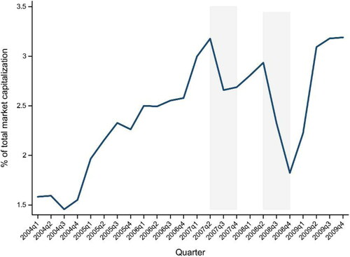
Around the global financial crisis of 2007–2009, hedge funds, which are considered informed and sophisticated arbitrageurs, simultaneously exited the market after the financial sector experienced an exceptionally large shock.¹ Ben-David et al. (2012) extensively examine prior research on hedge funds around the global financial crisis and state that ‘hedge funds exited the U.S. stock market en masse as the financial crisis evolved, primarily in response to the tightening of funding by investors and lenders.’ Their empirical evidence indicates that hedge funds reduced their equity holdings by 6% each quarter during the Quant Meltdown of 2007 and by 15% on average (29% with compounding) during Lehman Brothers’ bankruptcy in 2008 (see Figure 1). Ben-David et al. (2012) report that a quarter of all hedge funds sold over 40% of their equity holdings during 2008:Q3–Q4. He et al. (2010) similarly find that hedge funds reduced their holdings of securitized assets by $800 billion during the global financial crisis (2007:Q4–2009:Q1). Ang et al. (2011) examine data from December 2004 to October 2009 and find that hedge funds began to decrease their leverage even before the financial crisis started in mid-2007. In determining the primary motivation for this massive asset liquidation, Ben-David et al. (2012) point out that fund withdrawals explain half of the decline in hedge funds’ equity holdings. Holding enough cash during a crisis period is important because of its close relationship to a fund’s performance. Cao et al. (2013) show that most fund managers adjust their portfolios’ market exposures to mitigate aggregate liquidity shocks. They claim that good liquidity timers earn significantly higher returns. Agarwal et al. (2019) argue that hedge funds with illiquid assets are highly exposed to investor runs and perform poorly during a crisis (see also Chen et al. (2010) and Goldstein et al. (2017)). They show that funds increase their cash buffers to mitigate liquidity shocks (Zeng, 2017).

Figure 1. Fraction of U.S. stock market capitalization held by hedge funds.

The shaded areas are the quarters around the Quant Meltdown (2007:Q3–Q4) and Lehman Brothers’ bankruptcy (2008:Q3–Q4).

Source: Ben-David, Franzoni, and Moussawi (2012).

During a crisis, the market is subject to funding liquidity shocks because uninformed fund investors prudently request early withdrawals based on their own market views, which are shaped by managers giving up their market investments in aggregate. These investors can be viewed as similar to those described by Shleifer and Vishny (1997), who determine investment decisions based on past information about funds. The possibility of synchronized runs across various financial sectors has historically been of great concern to market participants, policymakers, and researchers.² Previous studies attempt to derive a unique equilibrium threshold for panic-based runs using global game methods. Goldstein and Pauzner (2004) define panic-based crises as ‘crises that occur just because agents believe they are going to occur’; this definition describes most crises in the financial sector. Goldstein and Pauzner (2005) modify Diamond and Dybvig (1983) bank run model to demonstrate the existence of a unique bank run equilibrium and calculate the probability of a bank run. Extending Goldstein and Pauzner’s model, Allen et al. (2018) investigate the economic effects of government guarantees on the banking system. Abreu and Brunnermeier (2002, 2003) identify long-lasting unexploited arbitrage opportunities in asset markets due to arbitrageurs’ failure to synchronize. Goldstein and Pauzner (2004) explain that crisis contagion between two financial markets with common investors may be due to fear of a crisis, which can cause investors to withdraw capital from both markets. Liu and Mello (2011) highlight fund investors’ synchronized withdrawals as a significant driver of the massive asset liquidation during the global financial crisis. They connect the limits to arbitrage to liquidity risk and conclude that fund managers who are subject to liquidity risk reduce their proportions of risky assets in preparation for fund runs.

However, most studies assume that fixed short-term asset returns are unrelated to agents’ investment decisions.³ Therefore, they fail to explain market crashes caused by investors who collectively liquidate their risky assets in fear of other investors’ liquidations. For example, Liu and Mello (2011) consider an isolated fund that does not interact with the market or other funds and focus on fund-specific rather than economy-wide characteristics. Thus, in their study, the link between fund runs and price reduction is weak, and they infer the influence of fund managers’ decisions on the financial market only indirectly. Regarding these issues, a large body of literature on the limits to arbitrage finds theoretical evidence that the asset fire sales of constrained arbitrageurs cause a price divergence. In a pioneering work, Shleifer and Vishny (1997) argue that arbitrageurs may abandon their arbitrage strategies under a performance-based compensation structure. If uninformed investors choose rewards and punishments in accordance with short-term fund performance, fund managers become myopic, leaving arbitrage opportunities unexploited. Gromb and Vayanos (2002), Liu and Longstaff (2004), and Brunnermeier and Pedersen (2009) develop a model in which arbitrageurs cannot pursue arbitrage profits because of margin constraints on collateralized assets. When arbitrageurs face collateral constraints, their arbitrage positions are limited. Consequently, market and funding illiquidity reinforce each other, creating liquidity spirals in which illustrate the connection between funding liquidity shocks and negative market returns (Ben-David et al., 2012; Boyson et al., 2010; Hanson & Sunderam, 2014; Teo, 2011). Furthermore, Liu and Mello (2011) assume that fund investors are informed and sophisticated and model a fund investor game. However, some studies argue that fund investors are not usually rational, especially in a distressed market. For example, Ben-David et al. (2012) find empirical evidence that during the global financial crisis, hedge fund investors actively withdraw capital from poorly performing funds, implying that investors make investment decisions depending on funds’ past information rather than on information regarding their future.

In this study, we model a game involving fund managers, who are known to be informed and sophisticated. In particular, we develop a market model to explain synchronized market runs by informed and rational fund managers. In our model, market prices and investment payoffs are endogenously determined by fund managers’ optimal investment strategies. This setting is based on the relationship between funding liquidity and asset markets. Accordingly, fund managers interact with other funds through the market price and making two optimal decisions: asset allocations and whether to stay. Fund managers follow simple optimal decision rules. At $t_1,$ managers choose the optimal asset allocation to maximize their final investment payoffs, and, at $t_2,$ they optimally choose whether to stay in the market based on their observed private signals. Fund managers interact with the market price; the market price rises, benefitting all managers, as managers invest more capital, and vice versa. When the market is in a ‘bad’ state (i.e., a state in which runs are possible), fund managers also interact by deciding whether to stay because investors request capital withdrawals in proportion to the number of exiting funds. Thus, each fund’s investment decision affects the other funds’ investment payoffs and, therefore, clearly affects their optimal decisions.

As a result, fund managers should take into account not only market conditions but also runs by other managers in determining their optimal strategies. As more fund managers decide to exit the market, the expected investment payoff of the remaining funds diminishes faster than that of the exiting funds, which may encourage the remaining funds to run. We consider the situation in which all funds choose to exit owing to the fear of runs even if economic conditions are not that bad (i.e., panic-based market runs). Using Carlsson and Van Damme (1993) global game method, we show that a unique threshold strategy exists in which no managers run if the liquidity shock is below the threshold, but all managers run otherwise. Having established this unique threshold strategy, we compare the optimal levels of market exposure in state I, in which runs are impossible, and state II, in which runs are possible. This comparison shows that when fund managers consider the possibility of a run, it is optimal for them to decrease their market exposure. In addition, we calculate the ex-ante probability of a market run, which is related to the distribution of funding liquidity shocks, by summing the probabilities over the range in which a market run is possible. Through this analysis, we find that the likelihood of a run rises as both funds’ market exposure and investors’ sensitivity to negative shocks increase.

In the framework of this model, we show that low levels of noise in private liquidity shock signals can lead to panic-based market runs not because of liquidity risk per se but because of the fear of a run. This approach allows us to identify a direct linkage between price reductions and fund managers’ decisions. This study helps to explain some stylized facts about fund manager behavior observed around the global financial crisis. Hedge funds, whose investors are highly sensitive to losses, are vulnerable to funding liquidity risk, and, thus, fund managers are cautious, holding more cash prior to crises. Nevertheless, if an exceptionally devastating liquidity shock sweeps the market, fund investors may start requesting capital withdrawals from their funds in response to the initial loss. Even if some fund managers know that the liquidity shock is not strong enough to exit the market, the fear of capital withdrawals and price reductions due to other funds running induces these managers to run as well. In the worst case, hedge funds collectively exit the market not because of risk itself but because of fear, which can explain hedge funds’ stock market exodus during the Quant Meltdown of 2007 and Lehman Brothers’ bankruptcy in 2008.

The remainder of this article is organized as follows. Section 2 describes the model settings. In Section 3, we find the equilibria in states I (in which runs are impossible) and II (in which runs are possible) and explore the effect of environmental changes on fund managers’ decisions. Section 4 summarizes and concludes the article.

2. Model

2.1. Main players

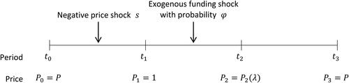
We consider a model with two assets, a risky asset and cash, spanning four periods ($t_0,t_1,t_2,t_3$). The risky asset market is subject to a negative price shock, and two types of agents participate in the market: fund managers and fund investors. Agents of the former type, fund managers, are homogeneous and fully rational with risk-neutral utility and know the fundamental value of the risky asset, which is higher than the current market price. Fund managers trade the risky asset to exploit arbitrage opportunities, but funding liquidity risk prevents them from earning maximum arbitrage profits. They make two decisions. First, they allocate their capital between the risky asset and cash. Second, they decide whether to stay in or exit from the risky asset market. Because there exist infinitely many fund managers⁴ who compete with each other in the market, individual fund managers optimally allocate their own capital across the risky asset and cash to maximize their final asset value in response to their competitors’ investment strategies in equilibrium. Agents of the latter type, fund investors, are uninformed and do not directly invest in the risky asset because the market is highly specialized and these investors are too prudent to invest by themselves. Instead, fund investors give their capital to fund managers, distributing it equally among all funds to reduce risk, and observe the funds’ aggregate investment decisions. Based on ex-post aggregate information about funds’ decisions, fund investors determine the amount of capital to withdraw in proportion to the aggregate proportion of exiting funds.

The brief time schedule of fund managers and investors proceeds as follows. At $t_1,$ fund investors provide aggregate capital $f,$ distributed equally among all funds. Fund $i$ then allocates a proportion $x_i$ of capital to the risky asset and the remaining proportion, $c_i,$ to cash, where $x_i\in [0,1].$ Cash pays a return of one unit, but the risky asset has an uncertain payoff in that fund managers’ decisions affect the market price. Risk-neutral fund managers’ optimal strategy is to maximize their expected final payoff; because the homogeneous fund managers, who know their peers’ optimal strategies, compete in the market, all managers select identical asset allocation strategies in equilibrium.⁵ Using this identity condition, we can assume that $x≔x_1=x_2=\dots =x{}_n.$ At t₂, each fund manager receives a funding liquidity shock with probability φ, where φ is uniformly distributed on $\left[0,1\right].$ The fund managers who receive this shock go bankrupt and earn no profits. Let $\theta$ be the proportion of defaulting funds. It follows that $\theta$= φ and that $\theta$ is also uniformly distributed on $\left[0,1\right].$ We call the remaining, non-defaulting funds the surviving funds, which comprise $1-\theta$ of all funds. Because an increase in $\theta$ reduces the remaining funds’ payoffs, fund managers are likely to exit the market when $\theta$ is high.

Surviving fund managers, however, do not know the exact value of $\theta$ because fund managers cannot observe the statuses of other funds, but rather, receive noisy signals. Specifically, the manager of surviving fund $i$ receives the signal ${\theta }_i=\theta +{\epsilon }_i,$ where ${\epsilon }_i$ is independent and identically uniformly distributed on the interval $\left[-\epsilon ,\epsilon \right]$ and $\epsilon$ is an arbitrarily small real number. Based on this signal, the manager of surviving fund $i$ forecasts the other managers’ strategies and decides whether to stay in the market. We denote $\lambda$ as the aggregate proportion of defaulting and exiting funds, and $\lambda -\theta$ is the proportion of surviving and exiting funds. After the surviving fund managers make their decisions, the fund investors observe $\lambda ,$ but they cannot distinguish which funds default or exit. We assume that they treat $\lambda$ as a proxy for the economic state and withdraw a proportion $g(\lambda )$ of their capital. $g(x)$ is an increasing function of $x$ because fund investors presume that a higher $\lambda$ implies a riskier market. For simplicity, we assume that $g\left(x\right)=x.$⁶ That is, fund investors withdraw precisely $\lambda$ of their capital from the remaining funds.

2.2. Determining the market price

Our model illustrates a distressed market in which the market price is below the fundamental price. We describe changes in the fundamental and market prices of the risky asset over time. For simplicity, we assume that the fundamental price P is time-invariant but that the market price diverges. At $t_0,$ the market price P₀ is equal to the fundamental price P. Between t₀ and t₁, a negative price shock occurs, reducing the market price by s. At $t_1,$ fund managers receive capital from investors and determine their investment strategies based on market conditions. After fund managers execute their investment strategies, the market price P₁ increases based on demand for the risky asset, which is calculated as $\frac{f}{n}{\sum }_{i=1}^n{x}_i=fx.$ For convenience, we normalize the market supply at $t_1$ to unity and express exogenous market factors, such as the market value, the amount of capital, and price shocks, relative to the price at $t_1.$ In addition, without loss of generality, we assume that the market price at $t_1$ equals one. Thus, the market price of the risky asset at t₁ is (1) $$\begin{array}{l}{P}_1=1=P-s+fx\\ P=1+s-fx,\end{array}$$(1) where $s$ is the impact of the negative market shock on the market price.

Between $t_1$ and $t_2,$ the market price decreases because of market fear. Allen and Gale (2004), Bernardo and Welch (2004), and Pedersen (2009) show that stock market investors overreact to negative price shocks and worsening market conditions during a financial crisis. We indicate investor sensitivity to the negative shock by $\tau ;$ that is, greater values of $\tau$ imply that market participants overreact to the negative shocks, and vice versa. We assume that the market price falls in response to past market returns; that is, because the market return of the risky asset changes from $P$ to 1 between $t_0$ and $t_1,$ the market price declines again between $t_1$ and $t_2.$ Specifically, it declines to $\frac{1}{P\tau },$ where $\tau \in [\frac{1}{P},1).$ The boundaries on $\tau$ restrict the impact of market fear such that $\frac{1}{P}<\frac{1}{P\tau }\le 1.$ The first inequality, $\frac{1}{P}<\frac{1}{P\tau },$ means that the effect of market fear does not dominate the market, meaning that the market price at t₂ does not fall below $\frac{1}{P}.$ The second inequality, $\frac{1}{P\tau }\le 1,$ limits the market price at t₂ to be less than or equal to one, focusing on only distressed markets.

The market price at t₂, denoted by P₂, is determined as follows. At t₂, fund investors withdraw a proportion $\lambda$ of their capital from the surviving funds. If the funds have enough cash, they do not have to sell any of their risky assets in response to these withdrawals. Thus, if $0\le \lambda \le c,$ market fear only affects the market price; that is, P₂ =$\frac{1}{P\tau }.$ However, if $\lambda$ is greater than $c,$ capital outflows are greater than funds’ cash holdings. Accordingly, the funds are forced to liquidate some of their risky assets, and P₂ decreases as a result. Notably, P₂ is a decreasing function of $\lambda ,$ and as $\lambda$ increases, funds are more likely to default. Let $\lambda {}_d$ be the largest value of $\lambda$ for which funds do not have to default; that is, funds default if $\lambda \ge \lambda {}_d$ and do not default otherwise. Then, if $c\le \lambda <\lambda {}_d,$ funds must sell $\frac{\lambda -c}{P{}_2}$ of their risky assets to prepare for a shortage of cash. For convenience, we index the $n$ funds such that the $m$ highest-indexed funds are the defaulting and exiting funds, that is, $\lambda =\frac{m}{n},$ and the remaining $n-m$ lower-indexed funds are the surviving funds. We also assume that buying or selling orders affect the market price in proportion to the current price. Then, the market price is determined as $P{}_2=\frac{1}{P\tau }-\mathrm{}{P}_2\mathrm{*}\frac{f}{n}*\left(n-m\right)*\frac{\lambda -c}{P{}_2}=\mathrm{}\frac{1}{P\tau }-\frac{n-m}{n}\left\{f\right(\lambda -c\left)\right\}.$ Finally, if $\lambda {}_d\le \lambda \le 1,$ all funds exit the market, and the market price is $P{}_2=\mathrm{}\frac{1}{P\tau }-\frac{n-m}{n}P{}_{2}x.$ Equation (2)(2) $$P_2\left(\lambda \right)=\{\begin{array}{ll}\frac{1}{P\tau },& 0\le \lambda <c\\ \frac{1}{P\tau }-\frac{n-m}{n}\left\{f\left(\lambda -c\right)\right\},& c\le \lambda <\lambda {}_d\\ \frac{1}{P\tau }-\frac{n-m}{n}P{}_{2}x,& \lambda {}_d\le \lambda \le 1\end{array}$$(2) summarizes the market price at t₂.⁸ (2) $$P_2\left(\lambda \right)=\{\begin{array}{ll}\frac{1}{P\tau },& 0\le \lambda <c\\ \frac{1}{P\tau }-\frac{n-m}{n}\left\{f\left(\lambda -c\right)\right\},& c\le \lambda <\lambda {}_d\\ \frac{1}{P\tau }-\frac{n-m}{n}P{}_{2}x,& \lambda {}_d\le \lambda \le 1\end{array}$$(2)

Note that fund investors’ cautious reactions to funding exits due to information asymmetry between fund managers and investors can stimulate runs on the remaining funds. Even a fund manager who knows that the funding liquidity shock is at a safe level may choose to exit if he or she thinks that other managers will leave the market, because other funds’ exits not only induce withdrawals but also lower market prices, reducing the remaining funds’ investment payoffs. If the payoff reduction seems to be severe enough, fund managers will decide to leave the market. After all, market runs can be triggered by the fear of runs, which leads to so-called panic-based market runs, regardless of market fundamentals. Eventually, at t₃, the market price P₃ converges to its fundamental value, P. Figure 2 briefly summarizes this time schedule.

Figure 2. Time schedule.

This graph summarizes the time schedule of the players and the change in the market price over time.

t₀: Market price P₀ is at the fundamental price P.

t₁: Each fund manager receives capital from investors and determines the proportion of risky asset x_i and cash c_i. Additionally, the market price diverges from the fundamental price P; P₁ = 1 = P–s + fx, where s is the impact of the negative price shocks.

t₂: Each fund manager decides whether to stay or exit. Then, fund investors observe λ and withdraw a proportion of λ from each fund. λ implies the proportion of defaulting and exiting funds.

t₃: Market price P₃ converges to the fundamental price P.

Source: The Authors.

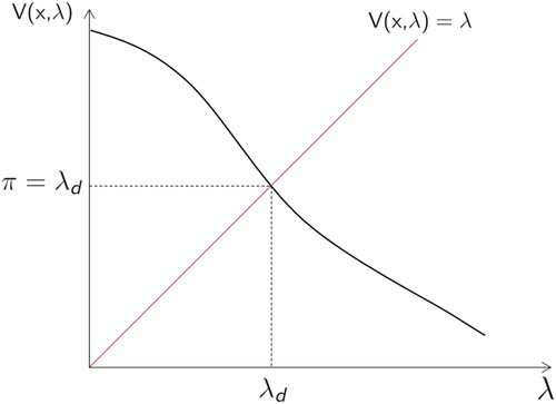
In our model, $\lambda {}_d$ plays an important role in fund maintenance. We now derive $\lambda {}_d$ and explain its economic meaning. Because fund managers sell the risky asset at price P₂, the liquidation value at t₂ is calculated as $V\left(x,\lambda \right)=xP{}_2\left(\lambda \right)+c.$ Thus, funds default when $\lambda >V$ and do not default when $\lambda \le V.$ We show that $P{}_2\left(\lambda \right)$ is a decreasing function of $\lambda ,$ implying that $V\left(x,\lambda \right)$ is as well. The graph of $V\left(x,\lambda \right)$ in Figure 3 shows that, in this case, $\lambda {}_d$ should satisfy $\lambda {}_d=V\left(x,{\lambda }_d\right).$ Furthermore, we can define the minimum value of the non-defaulting funds’ investment payoff before capital outflows, $\pi ,$ as in Equation (3)(3) $$\pi \mathrm{}:=V\left(x,\mathrm{}{\lambda }_d\right)=xP{}_2\left({\lambda }_d\right)+c=\mathrm{}\lambda {}_d$$(3) . Solving Equation (3)(3) $$\pi \mathrm{}:=V\left(x,\mathrm{}{\lambda }_d\right)=xP{}_2\left({\lambda }_d\right)+c=\mathrm{}\lambda {}_d$$(3) shows that $\pi =\frac{x}{P\tau (1+fx)}+c.$ (3) $$\pi \mathrm{}:=V\left(x,\mathrm{}{\lambda }_d\right)=xP{}_2\left({\lambda }_d\right)+c=\mathrm{}\lambda {}_d$$(3)

Figure 3. Graph of $V.$$\left(x,\lambda \right)$

This graph illustrates the decreasing function $V\left(x,\lambda \right)$ and the relationship between $\pi$ and ${\lambda }_d.$ Based on its definition, ${\lambda }_d$ should satisfy $\lambda {}_d=V\left(x,{\lambda }_d\right).$

Source: The Authors.

When a fund manager decides to exit the market, that fund earns an exit investment payoff ${\Pi }^E$ such that (4) $${\Pi }^E\left(x,\lambda \right)=\{\begin{array}{lll}x{P}_2\left(\lambda \right)+c& & 0\le \lambda <\pi \\ 0& & \pi \le \lambda \le 1\end{array}$$(4)

In Equation (4)(4) $${\Pi }^E\left(x,\lambda \right)=\{\begin{array}{lll}x{P}_2\left(\lambda \right)+c& & 0\le \lambda <\pi \\ 0& & \pi \le \lambda \le 1\end{array}$$(4) , ${\Pi }_i^E$ equals the investment payoff before capital outflows at t₂ if capital outflows are less than $\pi .$ Otherwise, the fund has no value, even if the fund manager decides to liquidate early.

When a fund manager decides to stay in the market, the investment payoff ${\Pi }_i^S$ for the fund is (5) $${\Pi }^S\left(x,\lambda \right)=\{\begin{array}{lll}xP+c-\lambda & & 0\le \lambda <c\\ xP-\left(\lambda -c\right)\frac{P}{P_2\left(\lambda \right)}& & c\le \lambda <\pi \\ 0& & \pi \le \lambda \le 1\end{array}$$(5)

In Equation (5)(5) $${\Pi }^S\left(x,\lambda \right)=\{\begin{array}{lll}xP+c-\lambda & & 0\le \lambda <c\\ xP-\left(\lambda -c\right)\frac{P}{P_2\left(\lambda \right)}& & c\le \lambda <\pi \\ 0& & \pi \le \lambda \le 1\end{array}$$(5) , if $\lambda$ is less than c, funds can cover all their outflows with cash at $t_2$ and obtain investment yield $xP$ from the risky asset at $t_3.$ If $\lambda$ is greater than c, the fund must liquidate the risky asset to cover the shortfall at $t_2,$ and thus suffers a loss of $\left(\lambda -c\right)\frac{P}{P_2}$ at $t_3.$ If $\lambda$ exceeds $\pi ,$ the fund manager defaults at $t_2.$

3. Equilibrium

In equilibrium, we can assume that $n\to \infty .$ Then, the fundamental and market prices and the investment payoffs of exiting and staying, given by Equations (1)(2) $$P_2\left(\lambda \right)=\{\begin{array}{ll}\frac{1}{P\tau },& 0\le \lambda <c\\ \frac{1}{P\tau }-\frac{n-m}{n}\left\{f\left(\lambda -c\right)\right\},& c\le \lambda <\lambda {}_d\\ \frac{1}{P\tau }-\frac{n-m}{n}P{}_{2}x,& \lambda {}_d\le \lambda \le 1\end{array}$$(2) , (2)(3) $$\pi \mathrm{}:=V\left(x,\mathrm{}{\lambda }_d\right)=xP{}_2\left({\lambda }_d\right)+c=\mathrm{}\lambda {}_d$$(3) , (4)(5) $${\Pi }^S\left(x,\lambda \right)=\{\begin{array}{lll}xP+c-\lambda & & 0\le \lambda <c\\ xP-\left(\lambda -c\right)\frac{P}{P_2\left(\lambda \right)}& & c\le \lambda <\pi \\ 0& & \pi \le \lambda \le 1\end{array}$$(5) , and (5)(6) $$\overline{P}≔\underset{n\to \mathrm{\infty }}{\lim }\left[P\right]=1+s-fx$$(6) , respectively, can be rewritten as follows. (6) $$\overline{P}≔\underset{n\to \mathrm{\infty }}{\lim }\left[P\right]=1+s-fx$$(6) (7) $$\overline{P_2}\left(\lambda \right)≔\underset{n\to \mathrm{\infty }}{\lim }\left[P_2\right]=\{\begin{array}{lll}\frac{1}{\overline{P}\tau }& & 0\le \lambda <c\\ \frac{1}{\overline{P}\tau }-f\left(\lambda -c\right)& & c\le \lambda <\pi \\ \frac{1}{\overline{P}\tau \left(1+fx\right)}& & \pi \le \lambda \le 1\end{array}\mathrm{}$$(7) (8) $$\overline{{\Pi }^E}\left(x,\lambda \right)≔\underset{n\to \mathrm{\infty }}{\lim }\left[{\Pi }^E\right]=\{\begin{array}{lll}\frac{x}{\overline{P}\tau }+c& & 0\le \lambda <c\\ \frac{x}{\overline{P}\tau }-fx\left(\lambda -c\right)+c& & c\le \lambda <\pi \\ 0& & \pi \le \lambda \le 1\end{array}$$(8) (9) $$\overline{{\Pi }^S}\left(x,\lambda \right)≔\underset{n\to \mathrm{\infty }}{\lim }\left[{\Pi }^S\right]=\{\begin{array}{lll}x\overline{P}+c-\lambda & & 0\le \lambda <c\\ x\overline{P}-\left(\lambda -c\right)\overline{P}/\left(\frac{1}{\overline{P}\tau }-f\left(\lambda -c\right)\right)& & c\le \lambda <\pi \\ 0& & \pi \le \lambda \le 1\end{array},$$(9) where $\pi =\frac{x}{\overline{P}\tau (1+fx)}+c.$ Furthermore, by differentiating ${\Pi }^E$ and ${\Pi }^S$ with respect to $x,$ we obtain the following equations: (10) $$\frac{\partial \overline{{\Pi }^E}}{\partial x}\left(x,\lambda \right)≔\underset{n\to \mathrm{\infty }}{\lim }\left[\frac{\partial {\Pi }^E}{\partial \mathrm{x}}\right]=\{\begin{array}{lll}\frac{1}{\overline{P}\tau }-1& & 0\le \lambda \le c\\ \frac{1}{\overline{P}\tau }-f\left(\lambda -c\right)-1& & c\le \lambda <\pi \\ 0& & \pi \le \lambda \le 1\end{array}\mathrm{}$$(10) (11) $$\frac{\partial \overline{{\Pi }^S}}{\partial x}\left(x,\lambda \right)≔\underset{n\to \mathrm{\infty }}{\lim }\left[\frac{\partial {\Pi }^S}{\partial \mathrm{x}}\right]=\{\begin{array}{lll}\overline{P}-1& & 0\le \lambda <c\\ \overline{P}-\overline{P}/\left(\frac{1}{\overline{P}\tau }-f\left(\lambda -c\right)\right)& & c\le \lambda <\pi \\ 0& & \pi \le \lambda \le 1\end{array}\mathrm{}$$(11)

3.1. State I: Runs are impossible

As the benchmark case, we first determine the equilibrium when surviving fund managers cannot exit the market. The only funds that exit are those that receive a liquidity shock. Thus, $\lambda$ equals $\theta .$ Under this condition, panic-based market runs are impossible because no surviving fund manager fears that other survivors will exit. Thus, the investment payoff of the surviving funds is the investment return ${\Pi }^S$ of staying, and the bankrupt funds obtain no payoffs. The expected final payoff of the surviving funds at $t_1,$ denoted by $E\left[{\Pi }^I\right],$ is therefore (12) $$E\left[{\Pi }^I\right]={\int }_0^1\left[\left(1-\phi \right)E\left[{\Pi }^S\right]\right]d\phi =E\left[{\Pi }^S\right]{\int }_0^1\left(1-\phi \right)d\phi =\frac{1}{2}E\left[{\Pi }^S\right]=\frac{1}{2}{\int }_0^{\pi }{\Pi }^{S}d\theta .\mathrm{}$$(12)

The fund managers choose their optimal market exposure to maximize $E\left[{\Pi }^I\right],$ that is, (13) $$\underset{x}{\max }E\left[{\Pi }^I\right]\mathrm{}$$(13) under the boundary conditions (14) $$0\le x\le 1,1/\tau \le P,f<s.$$(14)

The first boundary condition indicates the short-selling and borrowing constraints on the investment. The second boundary condition is imposed by the restriction on $\tau$ and guarantees the existence of an arbitrage opportunity because $1<1/\tau \le P$ is sufficient for $1<P.$ The third boundary condition excludes the possibility that a fund’s own investment is sufficient to cancel out a market shock.

In equilibrium, all fund managers choose the same optimal point, which should satisfy the equation (15) $$\frac{\partial E\left[{\Pi }^I\right]}{\partial x}≔\underset{n\to \mathrm{\infty }}{\lim }\left[\frac{\partial {\Pi }^I}{\partial \mathrm{x}}\right]=\frac{1}{2}\underset{n\to \infty }{\lim }\left[\frac{\partial }{\partial \mathrm{x}}\left({\int }_0^{\pi }{\Pi }^{S}d\theta \right)\right]=0.$$(15)

Theorem 1.

If surviving fund managers cannot exit the market, a panic-based market run cannot occur, and, in equilibrium, fund managers select the optimal market exposure $x^{I\mathrm{*}}$ that satisfies $\frac{1}{2}\left[f{x^{I\mathrm{*}}}^2-\left(f+s\right)x^{I\mathrm{*}}+s+\frac{x^{I\mathrm{*}}}{\left(1+f{x}^{I\mathrm{*}}\right)\tau }-\frac{1+s-f{x}^{I\mathrm{*}}}{f}\ln \left(1+f{x}^{I\mathrm{*}}\right)\right]=0.$

According to Theorem 1, when $x>x^{I*},$ fund managers can reduce the probability of a panic-based market run, but the funds’ expected payoff may fall. In contrast, when $x<x^{I*},$ the probability of a panic-based market run increases, and the funds’ expected payoff falls. Consequently, at $t_1,$ all fund managers decide to invest a proportion $x^{I*}$ of their capital in the market and to hold the remaining proportion $c^{I*}(=1-x^{I*})$ in cash. Then, the aggregate liquidity inflow from funds to the market is $f{x}^{I*},$ and the fundamental price is calculated as $P^{I*}=1+s-f{x}^{I*}$ accordingly.

At $t_2,$ after a proportion $\theta \mathrm{}(=\lambda )$ of funds exit the market owing to the liquidity shock, the market price of the risky asset at t₂ becomes (16) $$P_2^{I\mathrm{*}}\left(\theta \right)=\{\begin{array}{lll}\frac{1}{P^{I\mathrm{*}}\tau }& & 0\le \theta <c^{I\mathrm{*}}\\ \frac{1}{P^{I\mathrm{*}}\tau }-f\left(\theta -c\right)& & c^{I\mathrm{*}}\le \theta <{\pi }^{I\mathrm{*}}\\ \frac{1}{P^{I\mathrm{*}}\tau }-f\overline{P_2}x& & {\pi }^{I\mathrm{*}}\le \theta \le 1\end{array},$$(16) where ${\pi }^{I*}=\frac{x^{I*}}{P^{I*}\tau (1+f{x}^{I*})}+c^{I*}.$ In addition, the surviving funds can achieve investment return ${\Pi }^{I*}$ at $t_3,$ as follows: (17) $${\Pi }^{I\mathrm{*}}\left(x^{I\mathrm{*}},\theta \right)=\{\begin{array}{lll}{x}^{I\mathrm{*}}{P}^{I\mathrm{*}}+c^{I\mathrm{*}}-\theta & & 0\le \theta <c^{I\mathrm{*}}\\ x^{I\mathrm{*}}{P}^{I\mathrm{*}}-\left(\theta -c^{I\mathrm{*}}\right)\frac{P^{I\mathrm{*}}}{P_2^{I\mathrm{*}}}& & c^{I\mathrm{*}}\le \theta <{\pi }^{I\mathrm{*}}\\ 0& & {\pi }^{I\mathrm{*}}\le \theta \le 1\end{array}.$$(17)

3.2. State II: Runs are possible

We now consider the case in which the surviving funds can exit if the investment return from exiting the market seems greater than the investment return from staying. In this case, the proportion of exiting funds is equal to or greater than the proportion of bankrupt funds, meaning that $\lambda \ge \theta .$ In this section, we show that panic-based market runs can occur in the financial market as a result of rational fund managers’ optimal decisions. To do so, we use a global game method.

For technical reasons, we assume two dominance regions; fund managers who believe that $\theta$ is in one of these regions follow a dominance strategy regardless of what the other managers do. Specifically, managers who believe that $\theta$ is less than $\underset{\_}{\theta }$ choose to stay in the market. Here, $\underset{\_}{\theta }>2\epsilon ,$ and $[0,\underset{\_}{\theta })$ is the lower dominance region. To guarantee the existence of this region, the fund manager’s payoff structure requires some minor adjustments. Suppose that, if fund managers stay in the market when $\theta$ is in $[0,\underset{\_}{\theta }),$ they can obtain the investment return $x\overline{R}+c$ instead of $\overline{{\Pi }^S}.$ Then, regardless of the other managers’ decisions, these managers, who believe that $\theta$ is in $[0,\underset{\_}{\theta }),$ decide to stay because their investment return, $x\overline{R}+c,$ is independent of $\lambda$ and greater than $\overline{{\Pi }^E}.$ This result implies that when the liquidity shock is extremely weak, fund managers obtain higher investment profits by maintaining their current market position with certainty, regardless of other managers’ behavior.

At the other extreme, if fund managers believe that $\theta$ is greater than $\overline{\theta },$ they decide to exit the market, with $\overline{\theta }<\pi -2\epsilon .$ $(\overline{\theta },1]$ is therefore the upper dominance region. We first consider the clear case in which $\theta$ is in $[\pi ,1].$ In this case, all funds should exit the market with certainty because funds that stay in the market will be in default. In the second case, when $\theta$ is in $(\underset{\_}{\theta },\pi ),$ the surviving funds decide whether to stay based on the situation. Here, fund managers compare the investment returns $\overline{{\Pi }^E}$ and $\overline{{\Pi }^S}$ of each decision, and we need to demonstrate the existence of a unique value $\lambda$ in $[c,\pi ]$ for which $\overline{{\Pi }^E}$ and $\overline{{\Pi }^S}$ are equal. From Equations (8)(8) $$\overline{{\Pi }^E}\left(x,\lambda \right)≔\underset{n\to \mathrm{\infty }}{\lim }\left[{\Pi }^E\right]=\{\begin{array}{lll}\frac{x}{\overline{P}\tau }+c& & 0\le \lambda <c\\ \frac{x}{\overline{P}\tau }-fx\left(\lambda -c\right)+c& & c\le \lambda <\pi \\ 0& & \pi \le \lambda \le 1\end{array}$$(8) and (9)(9) $$\overline{{\Pi }^S}\left(x,\lambda \right)≔\underset{n\to \mathrm{\infty }}{\lim }\left[{\Pi }^S\right]=\{\begin{array}{lll}x\overline{P}+c-\lambda & & 0\le \lambda <c\\ x\overline{P}-\left(\lambda -c\right)\overline{P}/\left(\frac{1}{\overline{P}\tau }-f\left(\lambda -c\right)\right)& & c\le \lambda <\pi \\ 0& & \pi \le \lambda \le 1\end{array},$$(9) , we know that $\overline{{\Pi }^E}\left(x,c\right)<\overline{{\Pi }^S}\left(x,c\right),$ $\underset{\lambda \to \pi -0}{\lim }\overline{{\Pi }^E}\left(x,\lambda \right)>\overline{{\Pi }^S}\left(x,\pi \right)=0,$ and $\overline{{\Pi }^E}$ and $\overline{{\Pi }^S}$ decrease monotonically in $\lambda .$ Then, by the intermediate value theorem, a unique value of $\lambda$ exists that satisfies $\overline{{\Pi }^E}=\overline{{\Pi }^S}.$ If we define $\overline{\theta }$ as this value of $\lambda ,$ we can conclude that fund managers know that, in the region $(\underset{\_}{\theta },\pi ),$ exiting the market is more profitable than staying regardless of what the other managers do.

Now, to determine a unique equilibrium strategy in the lower dominance region, we consider the manager of fund $i,$ who receives a signal ${\theta }_i$ that is below $\underset{\_}{\theta }-\epsilon .$ This manager knows that $\theta$ is in the lower dominance region and decides to stay in the market. We are therefore assured that if $\theta$ is below $\underset{\_}{\theta }-2\epsilon ,$ all surviving fund managers receive signals in $[0,\underset{\_}{\theta }-\epsilon ),$ and no surviving manager chooses to exit. Thus, $\lambda =\theta$ when $\theta <\underset{\_}{\theta }-2\epsilon ,$ meaning that, in this region, only one equilibrium strategy exists. In the region $[\underset{\_}{\theta }-2\epsilon ,\underset{\_}{\theta }],$ as $\theta$ approaches $\underset{\_}{\theta },$ the proportion of managers who receive signals below $\underset{\_}{\theta }-\epsilon$ diminishes monotonically and equals zero at $\theta =\underset{\_}{\theta }.$

Similarly, we can also demonstrate the existence of a unique equilibrium strategy in the upper dominance region; fund manager $i$ chooses to exit if ${\theta }_i>\overline{\theta }+\epsilon ,$ meaning that $\lambda =1$ when $\theta >\overline{\theta }+2\epsilon .$ We now investigate what happens in the intermediate region between the two dominance regions. A fund manager who receives a signal slightly higher than $\underset{\_}{\theta }-\epsilon$ may think that $\theta$ is more likely to be in the lower dominance region and could decide to stay. However, as this private signal approaches $\underset{\_}{\theta },$ the probability that $\theta$ is in $[0,\underset{\_}{\theta })$ decreases to zero. At ${\theta }_i=\underset{\_}{\theta },$ the manager of fund $i$ knows that no manager has received a signal below $\underset{\_}{\theta }-\epsilon$ and that no manager can be sure that $\theta$ is in $[0,\underset{\_}{\theta }).$ Nevertheless, the manager of fund $i$ may choose to stay because he or she believes that other managers whose signals are lower than $\underset{\_}{\theta }$ may also choose to stay. The next manager, whose signal is slightly higher than that of the manager of fund $i,$ also believes that other managers may choose to stay and decides to stay as well. By applying this logic repeatedly to the subsequent managers, we can extend the region in which fund managers decide to stay too far above $\underset{\_}{\theta }.$ Similarly, the opposite situation, in which fund managers choose to exit because they believe that other managers will exit, can apply to the upper dominance region, and, thus, the region in which fund managers decide to exit can be extended to far below $\overline{\theta }.$ These two regions meet at a point ${\theta }^{*}$ in the middle of the intermediate region; at this point, every fund manager follows the strategy of staying if his or her signal is lower than ${\theta }^{*}$ and exiting otherwise. Thus, for a given private signal ${\theta }_i,$ the threshold strategy of the manager of fund $i$ at $t_2$ is (18) $$\left({\theta }_i,x\right)\to \{\begin{array}{cc}s\mathit{tay}& {\theta }_i<{\theta }^{\mathrm{*}}\left(x\right)\\ e\mathit{xit}& {\theta }^{\mathrm{*}}\left(x\right)\le {\theta }_i\end{array},$$(18) where the threshold ${\theta }^{*}(x)$ depends on the market exposure $x$ selected by the fund managers.

We now show that the threshold strategy in Equation (18)(18) $$\left({\theta }_i,x\right)\to \{\begin{array}{cc}s\mathit{tay}& {\theta }_i<{\theta }^{\mathrm{*}}\left(x\right)\\ e\mathit{xit}& {\theta }^{\mathrm{*}}\left(x\right)\le {\theta }_i\end{array},$$(18) has a unique equilibrium. Our approach is similar to Goldstein and Pauzner (2005) approach. First, we assume that all surviving fund managers follow the threshold strategy. Then, for a given threshold ${\theta }^{*}(x),$ the aggregate proportion of exiting funds $\lambda$ is determined to be the realized $\theta$ such that (19) $$\lambda \left(\theta ,{\theta }^{\mathrm{*}}\left(x\right)\right)=\{\begin{array}{lll}\theta & & 0\le \theta \le {\theta }^{\mathrm{*}}\left(x\right)-\epsilon \\ \theta +\left(1-\theta \right)\frac{\theta -\left({\theta }^{\mathrm{*}}\left(x\right)-\epsilon \right)}{2\epsilon }& & {\theta }^{\mathrm{*}}\left(x\right)-\epsilon \le \theta \le {\theta }^{\mathrm{*}}\left(x\right)+\epsilon \\ 1& & {\theta }^{\mathrm{*}}\left(x\right)+\epsilon \le \theta \le 1\end{array}.$$(19)

When $0\le \theta <{\theta }^{*}-\epsilon ,$ all surviving fund managers receive signals that are lower than ${\theta }^{*},$ and they all decide to stay. Similarly, when ${\theta }^{*}+\epsilon \le \theta \le 1,$ all signals are greater than ${\theta }^{*},$ and all managers choose to exit. When ${\theta }^{*}-\epsilon \le \theta \le {\theta }^{\mathrm{*}}+\epsilon ,$ the exiting funds include the bankrupt funds, corresponding to the proportion $\theta ,$ along with the surviving funds that choose to exit, which correspond to the proportion $\left(1-\theta \right)\frac{\theta -\left({\theta }^{*}-\epsilon \right)}{2\epsilon }.$

Next, we need to calculate the expected net investment returns of individual fund managers. We define $\Delta \overline{\Pi }\left(\lambda \right)$ as the net investment return from staying in the market rather than exiting: (20) $$\Delta \overline{\Pi }\left(\lambda \right)=\overline{{\Pi }^S}-\overline{{\Pi }^E}=\{\begin{array}{ll}x\overline{P}-\frac{x}{\overline{P}\tau }-\lambda & 0\le \lambda <c\\ x\overline{P}+\left(\lambda -c\right)\left[fx-\overline{P}/\left(\frac{1}{\overline{P}\tau }-f\left(\lambda -c\right)\right)\right]-\frac{x}{\overline{P}\tau }-c& c\le \lambda <\pi \\ 0& \pi \le \lambda \le 1\end{array}.$$(20)

In deciding whether to stay in the optimal investment decision, the manager of fund $i$ considers the expected net investment return, denoted by $E_{{\theta }_i,{\theta }^{*}}\left[\Delta \overline{\Pi }\right].$ If $E_{{\theta }_i,{\theta }^{*}}\left[\Delta \overline{\Pi }\right]$ is positive, the manager prefers to stay; otherwise, the manager exits. Because both $\theta$ and ${\epsilon }_i$ are uniformly distributed, $\theta$ is uniformly distributed over $\left[{\theta }_i-\epsilon ,{\theta }_i+\epsilon \right]$ from the perspective of the manager of fund $i,$ whose signal is ${\theta }_i=\theta +{\epsilon }_i.$ Thus, $E_{{\theta }_i,{\theta }^{*}}\left[\Delta \overline{\Pi }\right]$ can be calculated as (21) $$E_{{\theta }_i,{\theta }^{\mathrm{*}}}\left[\Delta \overline{\Pi }\right]=\frac{1}{2\epsilon }\underset{{\theta }_i-\epsilon }{\overset{{\theta }_i+\epsilon }{\int }}\Delta \overline{\Pi }\left(\lambda \left(\theta ,{\theta }^{\mathrm{*}}\right)\right)d\theta .\mathrm{}$$(21)

For a marginal fund manager whose signal is equal to the threshold ${\theta }^{*},$ the expected net investment return is zero, meaning that the marginal fund manager is indifferent between staying and exiting the market because the expected investment returns of both decisions are the same. Then, (22) $$E_{{\theta }^{*},{\theta }^{*}}\left[\Delta \overline{\Pi }\right]=\frac{1}{2\epsilon }\underset{{\theta }^{\mathrm{*}}-\epsilon }{\overset{{\theta }^{*}+\epsilon }{\int }}\Delta \overline{\Pi }\left(\lambda \left(\theta ,{\theta }^{*}\right)\right)d\theta =0.$$(22)

Using Equation (22)(21) $$E_{{\theta }_i,{\theta }^{\mathrm{*}}}\left[\Delta \overline{\Pi }\right]=\frac{1}{2\epsilon }\underset{{\theta }_i-\epsilon }{\overset{{\theta }_i+\epsilon }{\int }}\Delta \overline{\Pi }\left(\lambda \left(\theta ,{\theta }^{\mathrm{*}}\right)\right)d\theta .\mathrm{}$$(21) , we can show that a unique threshold equilibrium exists for a common threshold ${\theta }^{\mathrm{*}}.$ To prove that the threshold that satisfies Equation (22)(22) $$E_{{\theta }^{*},{\theta }^{*}}\left[\Delta \overline{\Pi }\right]=\frac{1}{2\epsilon }\underset{{\theta }^{\mathrm{*}}-\epsilon }{\overset{{\theta }^{*}+\epsilon }{\int }}\Delta \overline{\Pi }\left(\lambda \left(\theta ,{\theta }^{*}\right)\right)d\theta =0.$$(22) is unique, we must establish two dominance regions, which we have already done. As shown, in the lower dominance region, where ${\theta }^{*}<\underset{\_}{\theta }-\epsilon ,$ $E_{{\theta }_i,{\theta }^{*}}\left[\Delta \overline{\Pi }\right]$ is positive because fund managers always choose to stay regardless of the other managers’ decisions. Similarly, in the upper dominance region, if ${\theta }^{*}>\overline{\theta }+\epsilon ,$ $E_{{\theta }_i,{\theta }^{*}}\left[\Delta \overline{\Pi }\right]$ is negative. In addition, $E_{{\theta }_i,{\theta }^{*}}\left[\Delta \overline{\Pi }\right]$ is continuous and monotonically decreasing in ${\theta }^{*}$ between the two extreme regions. This monotonic decrease indicates that when ${\theta }_i$ and ${\theta }^{*}$ both increase by the same amount, although the marginal manager’s belief about the proportion of exits among surviving funds does not change, the manager believes that the proportion of bankrupt funds increases, leading to an increase in the aggregate proportion of exiting funds. The investment return of staying therefore decreases faster than that of exiting does. Thus, $E_{{\theta }_i,{\theta }^{*}}\left[\Delta \overline{\Pi }\right]$ is monotonically decreasing, and there exists a unique point ${\theta }^{\mathrm{*}}$ that satisfies $E_{{\theta }^{\mathrm{*}},{\theta }^{\mathrm{*}}}\left[\Delta \overline{\Pi }\right]=0.$ Unlike Goldstein and Pauzner (2005) model, in which the signal (i.e., the economy’s fundamentals) and the number of exiting agents are independent, our study shows that the two are closely related in that a higher signal indicates a stronger funding liquidity shock, which forces funds into bankruptcy and affects the investment returns of the surviving funds.

Finally, we need to show that the threshold strategy in Equation (18)(18) $$\left({\theta }_i,x\right)\to \{\begin{array}{cc}s\mathit{tay}& {\theta }_i<{\theta }^{\mathrm{*}}\left(x\right)\\ e\mathit{xit}& {\theta }^{\mathrm{*}}\left(x\right)\le {\theta }_i\end{array},$$(18) can be an equilibrium strategy. We therefore need to show that $E_{{\theta }_i,{\theta }^{*}}\left[\Delta \overline{\Pi }\right]$ is positive when ${\theta }_i<{\theta }^{\mathrm{*}}$ and negative when ${\theta }_i>{\theta }^{\mathrm{*}}.$ By the uniqueness of ${\theta }^{\mathrm{*}},$ we know that there exists only one point ${\theta }_i={\theta }^{\mathrm{*}}$ that satisfies $E_{{\theta }_i,{\theta }^{*}}\left[\Delta \overline{\Pi }\right]=0$ because ${\theta }^{\mathrm{*}}$ is a unique solution of $E_{{\theta }^{\mathrm{*}},{\theta }^{\mathrm{*}}}\left[\Delta \overline{\Pi }\right]=0.$ Suppose that the manager of fund $i$ receives the signal ${\theta }_i,$ which is lower than ${\theta }^{\mathrm{*}};$ then, the integral range of $E_{{\theta }_i,{\theta }^{\prime }}\left[\Delta \overline{\Pi }\right]$ is $\left[{\theta }_i-\epsilon ,{\theta }_i+\epsilon \right],$ which is below $\left[{\theta }^{\mathrm{*}}-\epsilon ,{\theta }^{\mathrm{*}}+\epsilon \right].$ From Equation (19)(19) $$\lambda \left(\theta ,{\theta }^{\mathrm{*}}\left(x\right)\right)=\{\begin{array}{lll}\theta & & 0\le \theta \le {\theta }^{\mathrm{*}}\left(x\right)-\epsilon \\ \theta +\left(1-\theta \right)\frac{\theta -\left({\theta }^{\mathrm{*}}\left(x\right)-\epsilon \right)}{2\epsilon }& & {\theta }^{\mathrm{*}}\left(x\right)-\epsilon \le \theta \le {\theta }^{\mathrm{*}}\left(x\right)+\epsilon \\ 1& & {\theta }^{\mathrm{*}}\left(x\right)+\epsilon \le \theta \le 1\end{array}.$$(19) , if $\theta <{\theta }^{\mathrm{*}},$ $\lambda \left(\theta ,{\theta }^{*}\right)<\lambda \left({\theta }^{*},{\theta }^{*}\right)$ implies that the integral of $\Delta \overline{\Pi }(\lambda (\theta ,{\theta }^{*}))$ over the range $\left[{\theta }_i-\epsilon ,{\theta }_i+\epsilon \right]$ is greater than that over the range $\left[{\theta }^{\mathrm{*}}-\epsilon ,{\theta }^{\mathrm{*}}+\epsilon \right]$ because $\Delta \overline{\Pi }(\lambda (\theta ,{\theta }^{*}))$ is decreasing in $\lambda .$ Thus, $E_{{\theta }_i,{\theta }^{*}}\left[\Delta \overline{\Pi }\right]>E_{{\theta }^{*},{\theta }^{*}}\left[\Delta \overline{\Pi }\right]=0$ when ${\theta }_i<{\theta }^{\mathrm{*}},$ meaning that the manager of fund $i$ decides to stay in the market. Similar logic can apply to the case in which ${\theta }_i>{\theta }^{\mathrm{*}}.$

Theorem 2.

A unique threshold equilibrium exists in which, for a common threshold ${\theta }^{\mathrm{*}},$ fund managers decide to stay in the market if the private signal is lower than ${\theta }^{\mathrm{*}}$ and decide to exit, leading to a run, if the private signal is greater than ${\theta }^{\mathrm{*}}.$

Theorem 2 implies that all fund managers make the same decision to stay or exit for a given market condition $\theta$ in equilibrium. This result is not surprising because fund managers affect each other through the asset price, and fund manager runs gradually reduce the other funds’ payoffs. Consequently, fear of a run drives fund managers to exit. Having established the existence of a unique threshold equilibrium, we now need to determine the actual threshold ${\theta }^{\mathrm{*}}(x).$ Liu and Mello (2011, p.497) state that as ‘$\epsilon \to 0,$ the fundamental uncertainty disappears, while strategic uncertainty remains unchanged.’ Applying their argument to our model, we know that $\lambda \left(\theta ,{\theta }^{*}\right)$ in Equation (19)(19) $$\lambda \left(\theta ,{\theta }^{\mathrm{*}}\left(x\right)\right)=\{\begin{array}{lll}\theta & & 0\le \theta \le {\theta }^{\mathrm{*}}\left(x\right)-\epsilon \\ \theta +\left(1-\theta \right)\frac{\theta -\left({\theta }^{\mathrm{*}}\left(x\right)-\epsilon \right)}{2\epsilon }& & {\theta }^{\mathrm{*}}\left(x\right)-\epsilon \le \theta \le {\theta }^{\mathrm{*}}\left(x\right)+\epsilon \\ 1& & {\theta }^{\mathrm{*}}\left(x\right)+\epsilon \le \theta \le 1\end{array}.$$(19) is uniformly distributed over the interval $\left[{\theta }^{\mathrm{*}},1\right]$ and that $\lambda \left(\theta ,{\theta }^{\mathrm{*}}\right)$ becomes a straight line over the interval $\left[{\theta }^{\mathrm{*}}-\epsilon ,{\theta }^{\mathrm{*}}+\epsilon \right]$ as $\epsilon \to 0.$ Thus, it is possible to identify ${\theta }^{\mathrm{*}}$ with the equation (23) $$\underset{{\theta }^{\mathrm{*}}}{\overset{1}{\int }}\Delta \overline{\Pi }\left(\lambda \right)d\lambda =0,$$(23) which results from transforming the variables in Equation (22)(22) $$E_{{\theta }^{*},{\theta }^{*}}\left[\Delta \overline{\Pi }\right]=\frac{1}{2\epsilon }\underset{{\theta }^{\mathrm{*}}-\epsilon }{\overset{{\theta }^{*}+\epsilon }{\int }}\Delta \overline{\Pi }\left(\lambda \left(\theta ,{\theta }^{*}\right)\right)d\theta =0.$$(22) by the linearity of $\lambda \left(\theta ,{\theta }^{*}\right).$ Figure 4 graphically specifies ${\theta }^{\mathrm{*}},$ which is determined at the point where the area of A (the region above the horizontal axis) is equal to that of B (the region below the horizontal axis). Using this result, we can determine the value of ${\theta }^{\mathrm{*}}(x)$ and the conditions for ${\theta }^{\mathrm{*}}(x)$ in the range $(c,\pi ).$

Figure 4. Net investment return from staying rather than exiting the market.

The net investment return from staying rather than exiting the market at t, $\Delta \overline{\Pi },$ is shown as a function of the aggregate proportion of exiting funds, $\lambda .$ Here, $f=4,$ $s=8,$ $\tau =0.3,$ and $x=0.71644.$

Source: The Authors.

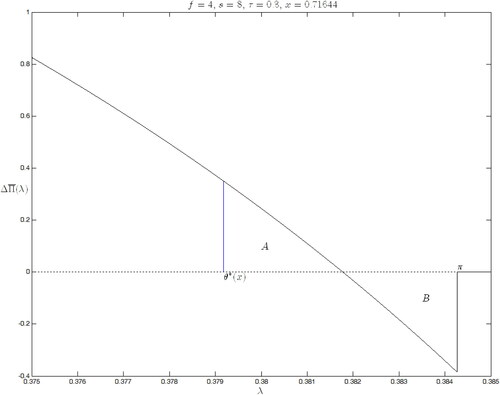
Theorem 3.

If $\frac{1}{f^2\tau }\left(fx-\ln f\right)>\frac{x}{(1+fx){\overline{R}}^2{\tau }^2}[\frac{x}{\overline{R}\tau }+\left(1+fx\right)c-\frac{f}{2}\left(\frac{x}{(1+fx)\overline{R}\tau }+2c\right)],$ then a unique threshold ${\theta }^{\mathrm{*}}(x)$ exists in the interval $(c,\pi ),$ and ${\theta }^{\mathrm{*}}(x)$ can be found by solving $\frac{1}{f^2\tau \left(\pi -{\theta }^{\mathrm{*}}\right)}\ln \left[(1+fx)(1-f\overline{R}\tau ({\theta }^{\mathrm{*}}-c)\right]=\frac{x}{\overline{R}\tau }-\frac{\left(1+fx\right)\overline{R}}{f}+\left(1+fx\right)c-\frac{f(\pi +{\theta }^{\mathrm{*}})}{2}.$⁹

Theorem 3 is the most important result of this study because it implies that when runs are possible, fund managers may exit even if the shock itself ($\theta$) is not sufficient to cause bankruptcy ($\pi$). The details are as follows. As $\epsilon \to 0,$ the aggregate proportion of exiting funds $\lambda$ in Equation (19)(19) $$\lambda \left(\theta ,{\theta }^{\mathrm{*}}\left(x\right)\right)=\{\begin{array}{lll}\theta & & 0\le \theta \le {\theta }^{\mathrm{*}}\left(x\right)-\epsilon \\ \theta +\left(1-\theta \right)\frac{\theta -\left({\theta }^{\mathrm{*}}\left(x\right)-\epsilon \right)}{2\epsilon }& & {\theta }^{\mathrm{*}}\left(x\right)-\epsilon \le \theta \le {\theta }^{\mathrm{*}}\left(x\right)+\epsilon \\ 1& & {\theta }^{\mathrm{*}}\left(x\right)+\epsilon \le \theta \le 1\end{array}.$$(19) becomes (24) $$\lambda \left(\theta ,{\theta }^{\mathrm{*}}\left(x\right)\right)=\{\begin{array}{ccc}\theta & & 0\le \theta \le {\theta }^{\mathrm{*}}\left(x\right)\\ 1& & {\theta }^{\mathrm{*}}\left(x\right)<\theta \le 1\end{array}.$$(24)

When $\theta$ is below the threshold ${\theta }^{\mathrm{*}}(x),$ all surviving fund managers decide to stay, but if $\theta$ is above ${\theta }^{\mathrm{*}}(x),$ all fund managers choose to exit the market. In contrast to state I, all fund managers exit the market in state II, even when $\theta$ is less than $\pi .$ If such a panic-based market run occurs, fund investors withdraw all their capital from fund managers. Thus, the managers of surviving funds cannot stay when $\theta \in ({\theta }^{\mathrm{*}},1].$ As a general condition, our interest in this study is the case that $c<{\theta }^{\mathrm{*}}<\pi .$ If ${\theta }^{\mathrm{*}}$ is below $c,$ panic-based market runs can occur even if fund managers prudently manage their assets and hold enough cash in preparation for a run. Thus, we exclude this case. Fund managers facing the risk of panic-based market runs consider ${\theta }^{\mathrm{*}}$ when deciding their optimal market exposure at $t_1.$ Thus, the optimal asset allocation problem of surviving fund manager $i$ is (25) $$\underset{x}{\max }E\left[{\Pi }^{II}\right],\mathrm{}$$(25) where $$E\left[{\Pi }_i^{II}\right]=\frac{1}{2}E\left[{\Pi }_i^S\right]=\frac{1}{2}{\int }_0^{{\theta }^{\mathrm{*}}\left(\mathrm{x}\right)}{\Pi }_i^{S}d\theta .$$

In the optimization problem of Equation (25)(24) $$\lambda \left(\theta ,{\theta }^{\mathrm{*}}\left(x\right)\right)=\{\begin{array}{ccc}\theta & & 0\le \theta \le {\theta }^{\mathrm{*}}\left(x\right)\\ 1& & {\theta }^{\mathrm{*}}\left(x\right)<\theta \le 1\end{array}.$$(24) , the integral range is $\left[0,{\theta }^{\mathrm{*}}(x_i)\right]$ because when ${\theta }^{*}\left(x\right)<\theta ,$ all fund managers choose to exit and investors withdraw all their capital, meaning that fund managers obtain zero investment returns. We consider the possible outcome if some fund managers remained in the market even in the range $\left[{\theta }^{*}\right(x),1].$ These remaining managers certainly can obtain positive rather than zero investment returns, but the other managers who chose to exit would make greater profits. Thus, rational fund managers prefer to exit, and, consequently, all fund managers choose to exit even if they know that they will obtain no investment payoff.

Now, we return to $t_1.$ In equilibrium, all fund managers choose the same optimal exposure $x^{II*},$ which satisfies (26) $$\frac{\partial E\left[{\Pi }^{II}\right]}{\partial x}≔\underset{n\to \mathrm{\infty }}{\lim }\left[\frac{\partial {\Pi }^{II}}{\partial x}\right]=\frac{1}{2}\underset{n\to \mathrm{\infty }}{\mathit{lim}}\left[\frac{\partial }{\partial x}\left({\int }_0^{{\theta }^{\mathrm{*}}\left(x\right)}{\Pi }^{S}d\theta \right)\right]=0.\mathrm{}$$(26)

Once $x^{II*}$ is determined at $t_1,$ the threshold strategy is that if $\theta$ is below ${\theta }^{*}\left(x^{II*}\right),$ all surviving funds stay in the market, but if not, all funds exit. Moreover, we can calculate the ex-ante probability of a market run. Given the assumption that $\theta$ is uniformly distributed over the interval $[0,1],$ the probability of runs is $p_{\mathit{run}}=1-{\theta }^{*}.$

In Section 3.3, we explore the effect of a panic-based market run on fund managers’ asset allocations and then investigate the change in the probability of a run in response to an unexpected change in $\tau .$

3.3. Effect of the possibility of a panic-based market run on fund asset allocations

When a panic-based market run can occur, the range in which funds survive changes from $\left[0,\pi \right]$ to $\left[0,{\theta }^{\mathrm{*}}\right].$ Then, the optimal $x^{I*}$ that maximizes $\frac{1}{2}{\int }_0^{\pi }{\Pi }_i^{S}d\theta$ in state I is no longer optimal when maximizing $\frac{1}{2}{\int }_0^{{\theta }^{\mathrm{*}}(x)}{\Pi }_i^{S}d\theta$ in state II. If a run is possible, fund managers subject to panic-based market runs choose their optimal asset allocations by considering the range of survival, $\left[0,{\theta }^{\mathrm{*}}\right].$ Thus, we investigate how fund managers’ optimal decisions change with the introduction of possible runs.

Because $x^{I*}$ and $x^{II*}$ are the solutions to the maximization problems in states I and II, respectively, they should satisfy ${\left[\frac{\partial E\left[{\Pi }^I\right]}{\partial x}\right]}_{x=x^{I*}}=0$ and ${\left[\frac{\partial E\left[{\Pi }^{II}\right]}{\partial x}\right]}_{x=x^{II*}}=0,$ respectively. Thus, if $x^{II*}<x^{I*},$ ${\left[\frac{\partial E\left[{\Pi }^{II}\right]}{\partial x}\right]}_{x=x^{I*}}$ is negative, but if $x^{II*}>x^{I*},$ ${\left[\frac{\partial E\left[{\Pi }^{II}\right]}{\partial x}\right]}_{x=x^{I*}}$ is positive. In this section, we show that $x^{II*}<x^{I*}$ by proving that ${\left[\frac{\partial E\left[{\Pi }^{II}\right]}{\partial x}\right]}_{x=x^{I*}}<0$ when ${\theta }^{\mathrm{*}}\in (c,\pi ).$

First, we compare the magnitudes of the integrals ${\int }_{{\theta }^{\mathrm{*}}}^{\pi }\frac{\partial \overline{{\Pi }^E}}{\partial x}d\lambda$ and ${\int }_{{\theta }^{\mathrm{*}}}^{\pi }\frac{\partial \overline{{\Pi }^S}}{\partial x}d\lambda .$ From Equations (10)(10) $$\frac{\partial \overline{{\Pi }^E}}{\partial x}\left(x,\lambda \right)≔\underset{n\to \mathrm{\infty }}{\lim }\left[\frac{\partial {\Pi }^E}{\partial \mathrm{x}}\right]=\{\begin{array}{lll}\frac{1}{\overline{P}\tau }-1& & 0\le \lambda \le c\\ \frac{1}{\overline{P}\tau }-f\left(\lambda -c\right)-1& & c\le \lambda <\pi \\ 0& & \pi \le \lambda \le 1\end{array}\mathrm{}$$(10) and (11)(11) $$\frac{\partial \overline{{\Pi }^S}}{\partial x}\left(x,\lambda \right)≔\underset{n\to \mathrm{\infty }}{\lim }\left[\frac{\partial {\Pi }^S}{\partial \mathrm{x}}\right]=\{\begin{array}{lll}\overline{P}-1& & 0\le \lambda <c\\ \overline{P}-\overline{P}/\left(\frac{1}{\overline{P}\tau }-f\left(\lambda -c\right)\right)& & c\le \lambda <\pi \\ 0& & \pi \le \lambda \le 1\end{array}\mathrm{}$$(11) , we know that in the interval $c\le \lambda <\pi ,$ $\frac{\partial \overline{{\Pi }^E}}{\partial x}=\overline{P_2}-1$ and $\frac{\partial \overline{{\Pi }^S}}{\partial x}=\frac{\overline{P}}{P_2}\left(\overline{P_2}-1\right).$ Because $\overline{P}>1>\overline{P_2},$ $\frac{\partial \overline{{\Pi }^S}}{\partial x}<\frac{\partial \overline{{\Pi }^E}}{\partial x}<0.$ The integrals of both formulas over the range $[{\theta }^{\mathrm{*}},\pi ]$ also obey this dominance relation, implying that ${\int }_{{\theta }^{\mathrm{*}}}^{\pi }\frac{\partial \overline{{\Pi }^S}}{\partial x}d\lambda <{\int }_{{\theta }^{\mathrm{*}}}^{\pi }\frac{\partial \overline{{\Pi }^E}}{\partial x}d\lambda <0.$

Lemma 1.

${\int }_{{\theta }^{\mathrm{*}}}^{\pi }\frac{\partial \overline{{\Pi }^S}}{\partial x}d\lambda <{\int }_{{\theta }^{\mathrm{*}}}^{\pi }\frac{\partial \overline{{\Pi }^E}}{\partial x}d\lambda <0.$

Lemma 1 implies that on the interval $[{\theta }^{\mathrm{*}},\pi ],$ for a given increase in investment, the sum of the marginal losses is greater for funds that stay than that for funds that exit when $\lambda$ is expected to be in the range in which a market run can occur. This is because, in the interval $c\le \lambda <\pi ,$ we know that $\frac{\partial \overline{{\Pi }^S}}{\partial x}<\frac{\partial \overline{{\Pi }^E}}{\partial x}<0;$ this inequality means that, for a given increase in investment, the loss of returns from staying in the market is greater than the loss from exiting.

From Equation (23)(23) $$\underset{{\theta }^{\mathrm{*}}}{\overset{1}{\int }}\Delta \overline{\Pi }\left(\lambda \right)d\lambda =0,$$(23) , we know that ${\int }_{{\theta }^{\mathrm{*}}}^{\pi }\overline{{\Pi }^E}d\lambda ={\int }_{{\theta }^{\mathrm{*}}}^{\pi }\overline{{\Pi }^S}d\lambda ,$ and by differentiating both sides of the equation with respect to $x,$ we obtain Lemma 2.

Lemma 2.

$\frac{\partial {\theta }^{\mathrm{*}}(x)}{\partial x}=\frac{{\int }_{{\theta }^{\mathrm{*}}}^{\pi }\frac{\partial \overline{{\Pi }^S}}{\partial x}d\lambda -{\int }_{{\theta }^{\mathrm{*}}}^{\pi }\frac{\partial \overline{{\Pi }^E}}{\partial x}d\lambda }{\overline{{\Pi }^S}\left(x,{\theta }^{\mathrm{*}}\right)-\overline{{\Pi }^E}\left(x,{\theta }^{\mathrm{*}}\right)}$

Lemma 1 implies that the numerator on the right-hand side of the equation in Lemma 2 is negative, and the denominator, $\overline{{\Pi }^S}\left(x,{\theta }^{*}\right)-\overline{{\Pi }^E}\left(x,{\theta }^{*}\right),$ is positive because, at $\lambda ={\theta }^{\mathrm{*}},$ the investment return from staying is greater than the investment return from exiting, leading to the result that $\frac{\partial {\theta }^{\mathrm{*}}(x)}{\partial x}<0.$

Theorem 4.

The threshold ${\theta }^{\mathrm{*}}(x)$ is a decreasing function of market investment $x$ under the general condition that $c<{\theta }^{\mathrm{*}}(x)\mathrm{}<\pi .$ The probability of a market run, $p_{\mathit{run}},$ therefore increases as fund managers invest more in the market.

Because the probability of a market run is $p_{\mathit{run}}\left(x\right)=1-{\theta }^{*}\left(x\right),$ Theorem 4 states that $p_{\mathit{run}}$ is increasing in $x.$ When fund managers hold a large amount of the risky asset, their investment returns are closely related, and thus, funds respond sensitively to each other’s runs because fund exits reduce short-term market returns and stimulate fund withdrawals. In fact, fund exits lower the investment returns from both staying and exiting, but the remaining funds become more fragile than the exiting funds because the return from staying is rapidly diminished by the reduction in short-term market returns, and fund withdrawals affect only the remaining funds.¹⁰¹¹ Thus, if fund managers hold a large amount of the risky asset, they may choose to exit the market after observing a private signal; otherwise, they may choose to stay. In other words, funds behave more prudently when they hold more of the risky asset, meaning that ${\theta }^{*}$ decreases as $x$ increases. Hence, the probability of a market run rises as funds’ investments increase.

Using Lemmas 1 and 2, we can derive Lemma 3.

Lemma 3.

$x^{II\mathrm{*}}<x^{I\mathrm{*}}$ if and only if ${\left[\frac{\overline{{\Pi }^S}\left(x,{\theta }^{\mathrm{*}}\right)}{\overline{{\Pi }^E}\left(x,{\theta }^{\mathrm{*}}\right)}\right]}_{x=x^{I\mathrm{*}}}<{\left[\frac{{\int }_{{\theta }^{\mathrm{*}}}^{\pi }\frac{\partial \overline{{\Pi }^S}}{\partial x}d\lambda }{{\int }_{{\theta }^{\mathrm{*}}}^{\pi }\frac{\partial \overline{{\Pi }^E}}{\partial x}d\lambda }\right]}_{x=x^{I\mathrm{*}}}$

Lemma 3 explains the condition under which $x^{II*}<x^{I*}.$ Following Lemma 3, if ${\left[\frac{\overline{{\Pi }^S}\left(x,{\theta }^{*}\right)}{\overline{{\Pi }^E}\left(x,{\theta }^{*}\right)}\right]}_{x=x^{I*}}<{\left[\frac{{\int }_{{\theta }^{\mathrm{*}}}^{\pi }\frac{\partial \overline{{\Pi }^S}}{\partial x}d\lambda }{{\int }_{{\theta }^{\mathrm{*}}}^{\pi }\frac{\partial \overline{{\Pi }^E}}{\partial x}d\lambda }\right]}_{x=x^{I*}},$ fund managers optimally reduce their market exposure when they account for the possibility of a run. Under this condition, the left-hand side of the equation, $\frac{\overline{{\Pi }^S}\left(x,{\theta }^{*}\right)}{\overline{{\Pi }^E}\left(x,{\theta }^{*}\right)},$ is the ratio of the investment return of staying to that of exiting at $\lambda ={\theta }^{\mathrm{*}},$ and the right-hand side, $\frac{{\int }_{{\theta }^{\mathrm{*}}}^{\pi }\frac{\partial \overline{{\Pi }^S}}{\partial x}d\lambda }{{\int }_{{\theta }^{\mathrm{*}}}^{\pi }\frac{\partial \overline{{\Pi }^E}}{\partial x}d\lambda },$ is the ratio of the sum of marginal losses from an investment increase in the case of staying relative to that of exiting conditional on $\lambda$ being in the interval $[{\theta }^{\mathrm{*}},\pi ].$ Then, $\frac{\overline{{\Pi }^S}\left(x,{\theta }^{*}\right)}{\overline{{\Pi }^E}\left(x,{\theta }^{*}\right)}<\frac{{\int }_{{\theta }^{\mathrm{*}}}^{\pi }\frac{\partial \overline{{\Pi }^S}}{\partial x}d\lambda }{{\int }_{{\theta }^{\mathrm{*}}}^{\pi }\frac{\partial \overline{{\Pi }^E}}{\partial x}d\lambda }$ can be interpreted as the relative value of the sum of marginal losses on $\left[{\theta }^{*},\pi \right]$ being greater than the relative investment return at the threshold ${\theta }^{\mathrm{*}}.$ Thus, Lemma 3 predicts that when $\frac{\overline{{\Pi }^S}\left(x,{\theta }^{*}\right)}{\overline{{\Pi }^E}\left(x,{\theta }^{*}\right)}<\frac{{\int }_{{\theta }^{\mathrm{*}}}^{\pi }\frac{\partial \overline{{\Pi }^S}}{\partial x}d\lambda }{{\int }_{{\theta }^{\mathrm{*}}}^{\pi }\frac{\partial \overline{{\Pi }^E}}{\partial x}d\lambda },$ fund managers lose more money if they do not reduce their investments after the regime changes from state I to state II. Fund managers therefore prefer to hold cash when there is a risk of a market run. In our model, $\frac{\overline{{\Pi }^S}\left(x,{\theta }^{*}\right)}{\overline{{\Pi }^E}\left(x,{\theta }^{*}\right)}$ is bounded above by ${\overline{R}}^2\tau$ because $\frac{\overline{{\Pi }^S}\left(x,c\right)}{\overline{{\Pi }^E}\left(x,c\right)}$ is ${\overline{P}}^2\tau$ at $\lambda =c,$ and it monotonically decreases as $\lambda$ increases. Conversely, $\frac{{\int }_{{\theta }^{\mathrm{*}}}^{\pi }\frac{\partial \overline{{\Pi }^S}}{\partial x}d\lambda }{{\int }_{{\theta }^{\mathrm{*}}}^{\pi }\frac{\partial \overline{{\Pi }^E}}{\partial x}d\lambda }$ is bounded below by ${\overline{P}}^2\tau$ because $\left|\frac{\partial \overline{{\Pi }^S}}{\partial x}\right|$ is greater than ${\overline{P}}^2\tau ·\left|\frac{\partial \overline{{\Pi }^E}}{\partial x}\right|$ on $[{\theta }^{\mathrm{*}},\pi ].$ Thus, our model satisfies the condition in Lemma 3 and, when the regime changes from state I to state II, fund managers can maximize the expected value of their assets by reducing market exposure up to $x^{II*},$ meaning that $x^{II*}<x^{I*}.$ From Equations (8) and (11) and Lemma 3, we can derive the following theorem.

Theorem 5.

Fund managers decrease their market investments when they consider market runs in their optimal investment strategy; that is, $x^{II\mathrm{*}}<x^{I\mathrm{*}}.$

Theorem 5 is the main conclusion of this study. Indeed, around the global financial crisis, the regime suddenly changed from state I (i.e., runs are impossible) to state II (i.e., runs are possible). Hedge fund managers who perceived this regime change anticipated that market runs might aggravate the illiquidity problem and quickly reduced their market exposure even prior to the crisis. Nevertheless, as the crisis evolved, fund investors started to withdraw, and hedge funds began to liquidate in response to these withdrawals not because of systematic risk per se but because of the fear of others’ runs. Ultimately, as fear peaked following major financial events (i.e., the Quant Meltdown and Lehman Brothers’ bankruptcy), a mass exodus of hedge funds occurred; in other words, synchronized runs occurred owing to the extreme fear of runs.

Thus far, we have investigated the effect of investor sensitivity, $\tau ,$ on the probability of a market run, $p_{\mathit{run}}.$ A change in $\tau$ affects both P₂ and funds’ investment payoffs. Thus, if an unexpected change in $\tau$ occurs, then, for a given $x,$ fund managers adjust their existing threshold strategies to reflect the new $\tau .$ In turn, this adjustment changes the probability of a market run. Figure 5 illustrates this tendency for different levels of market exposure $x$ given the parameter values $f=4$ and $s=8.$ The horizontal axis represents $\tau ,$ which ranges from 0.2 to 0.9, and the vertical axis denotes $p_{\mathit{run}}.$ Because the boundary condition restricts $\tau$ to the range $[1/\overline{P},1),$ we exclude both upper and lower extreme values of $\tau .$ Each curve shows $p_{\mathit{run}}$ as a function of $\tau$ for different values of $x,$ which increase from 0.2 to 0.9 by increments of 0.1.

Figure 5. The probability of a market run.

This graph shows the probability of a market run, $p_{\mathit{run}},$ as a function of the price sensitivity, $\tau .$ Each curve illustrates the function for a different level of market exposure $x,$ ranging from 0.2 to 0.9. Here, $f=4$ and $s=8.$

Source: The Authors.

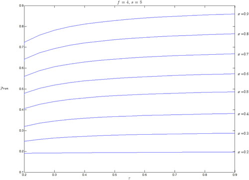
All the curves in Figure 5 are monotonically increasing, which indicates the fragility of a highly sensitive market. In a financial market in which investors respond sensitively to a negative shock, even moderate market shocks can greatly impact the market price, leading to a large price drop. The price reduction is more detrimental to staying funds than to exiting funds, implying that a highly sensitive market is more prone to suffer from market runs. To put it concretely, an increase in sensitivity $\tau$ decreases P₂ and, accordingly, $\overline{{\Pi }^S}$ falls more sharply than $\overline{{\Pi }^E}$ does. Because the net investment return function, $\Delta \overline{\Pi }\left(\lambda \right)=\overline{{\Pi }^S}-\overline{{\Pi }^E},$ decreases, the threshold ${\theta }^{\mathrm{*}}$ decreases because ${\theta }^{\mathrm{*}}$ satisfies ${\int }_{{\theta }^{\mathrm{*}}}^1\Delta \overline{\Pi }\left(\lambda \right)d\lambda =0$ (see Figure 4). Thus, in response to an unexpectedly high trend sensitivity $\tau ,$ fund managers lower the threshold ${\theta }^{\mathrm{*}},$ and the probability of a market run, $p_{\mathit{run}},$ increases. Goldstein and Pauzner (2005) and Liu and Mello (2011) similarly predict that short-term price reductions increase the possibility of a synchronized run. However, their results stem from the simple assumption of a constant short-term return because their models do not incorporate a price determination mechanism. In contrast, we develop a market model in which the short-term market return is endogenously determined by several factors; among them, we note that price sensitivity is an important factor that affects the probability of a market run. Because of this relationship, we suggest that lowering the information cost mitigates irrational fear in the market and could help resolve the synchronization problem in a distressed market by enhancing market stability.

4. Conclusion

Hedge funds have fragile capital structures because uninformed fund investors are highly sensitive to losses and are quick to withdraw their capital in response to bad news. Hedge fund managers, who share common investors and interact with each other through market prices, react sensitively to other funds’ investment decisions. In this environment, a panic-based market run can arise not because of systematic risk but merely because of the fear of a run. This study develops a market model to illustrate the synchronized market runs of informed and rational fund managers. Using a global game technique, we show that the possibility of a run can induce a panic-based market run not because of systematic risk itself but because of the fear of a run. In addition, we find that when the market regime changes from a normal state, in which runs are impossible, to a bad state, in which runs are possible, fund managers quickly reduce their exposure to risky assets prior to a run. By analyzing the ex-ante probability of a market run, we also suggest that a market in which fund managers are highly exposed to the market and participants are highly sensitive to negative shocks is more likely to experience synchronized runs. This study differs from existing studies in two ways. First, we consider the interaction between fund managers’ decisions and asset prices to address the relationship between funding liquidity and the stock market’s status. Furthermore, we illustrate a game between fund managers, who are known to be informed and sophisticated, rather than a game between fund investors. Thus, this study supplements the existing literature about fund runs and helps explain the commonly observed behavior of funds during a crisis.

Our findings provide some economic implications about fund managers’ behavior during a financial crisis. Hedge funds, whose investors are highly sensitive to losses, behave cautiously, holding more cash prior to a crisis. Nevertheless, as a financial crisis evolves, fund investors start to withdraw capital from their funds in response to the initial losses. Although fund managers who sufficiently reduce their exposure to risky assets in advance may know that a liquidity shock is not strong enough to pull them from the market, their growing fear of capital withdrawals and further price reductions caused by other funds’ runs could ultimately induce them to run as well. In the worst case, hedge funds may collectively exit the market not because of risk itself but because of fear, as observed during the Quant Meltdown of 2007 and Lehman Brothers’ bankruptcy in 2008. In such a scenario, high-volatility stocks are more likely to experience stronger fire sales than low-volatility stocks are because high-volatility stocks respond sensitively to price movements and are more likely to experience price drops during a market downturn.

Disclosure statement

No potential conflict of interest was reported by the author(s).

Additional information

Funding

This work was supported by the National Research Foundation of Korea (NRF) grant funded by the Korea government (MSIT; Ministry of Science and ICT) [No. 2019R1G1A1100196].

Notes

1 According to Hedge Fund Research, Inc., about 1,500 hedge funds were liquidated in 2008, a historical high, and more than 1,000 hedge funds closed the in following year, a second historical high.

2 Diamond and Dybvig (1983), Postlewaite and Vives (1987), Green and Lin (2003), Peck and Shell (2003), Goldstein and Pauzner (2005), and Ennis & Keister, 2009b) discuss bank runs; Bernardo and Welch (2004) and Morris and Shin (2004) study market runs; and Liu and Mello (2011) investigate fund runs.

3 Morris and Shin (2004) develop a model in which investors’ decisions to stay or not can explain the market price dynamics. However, investors in their model are not subject to early withdrawals, which are the core driver of market runs in our model; instead, they are constrained by loss limits.

4 We assume that the market is perfectly competitive, that is, it has infinitely many funds. However, for ease of presentation, we describe our model in this section as if the market included $n$ funds. Later, we allow $n$ to go to infinity.

5 This result is a Nash equilibrium.

6 It may be unrealistic to assume that withdrawals have a one-to-one correspondence with the aggregate proportion of defaulting and exiting funds. Adopting a complex function or considering heterogeneous investor decisions are interesting directions for further research.

8 To solve the model analytically, we assume that new liquidity inflows into the risky asset market at $t_2$ cancel out liquidity outflows from defaulting funds; however, this assumption does not change the model implications because the negative relation between liquidity outflows and market returns is maintained.

9 Proofs are provided in the Appendix.

10 Fund withdrawals indirectly affect the investment return from exiting through short-term price reductions.

11 Fund withdrawals indirectly affect the investment return from exiting through short-term price reductions.

12 If $g(y,z)$ and its partial derivative $g_y(y,z)$ are both continuous over $[y_0,y_1]\times [z_0,z_1],$ then $\frac{\partial }{\partial y}\left({\int }_{z_0}^{z_1}g\left(y,z\right)dz\right)={\int }_{z_0}^{z_1}{g}_y(y,z)dz+g\left(y,z_1\right)\frac{\partial z_1}{\partial y}-g\left(y,z_0\right)\frac{\partial z_0}{\partial y}.$

Appendix

A.1 Proof of Theorem 1

Because ${\Pi }^S\left(x,\theta \right)$ is continuous over $[0,1]\times [0,1]$ and its partial derivative, $\frac{\partial }{\partial x}{\Pi }^S\left(x,\theta \right),$ is continuous over $[0,1]\times [0,c]$ and $[0,1]\times [c,\pi ],$ the Leibniz integral rule¹² can be used to express $\frac{\partial }{\partial x}\left({\int }_0^{\pi }{\Pi }^S\left(x,\theta \right)d\theta \right)$ in Equation (15)(14) $$0\le x\le 1,1/\tau \le P,f<s.$$(14) as $$\frac{\partial }{\partial x}\left({\int }_0^{\pi }{\Pi }^S\left(x,\theta \right)d\theta \right)=\frac{\partial }{\partial x}\left({\int }_0^c{\Pi }^S\left(x,\theta \right)d\theta \right)+\frac{\partial }{\partial x}\left({\int }_c^{\pi }{\Pi }^S\left(x,\theta \right)d\theta \right)=$$ $$\left[{\int }_0^c\frac{\partial }{\partial x}{\Pi }^S\left(x,\theta \right)d\theta +{\Pi }^S\left(x,c\left(x\right)\right)\frac{\partial c}{\partial x}-{\Pi }^S\left(x,0\right)\frac{\partial 0}{\partial x}\right]+$$ $$\left[{\int }_c^{\pi }\frac{\partial }{\partial x}{\Pi }^S\left(x,\theta \right)d\theta +{\Pi }^S\left(x,\pi \right)\frac{\partial \pi }{\partial x}-{\Pi }^S\left(x,c\left(x\right)\right)\frac{\partial c}{\partial x}\right].$$

It follows that $$\underset{n\to \mathrm{\infty }}{\lim }\frac{\partial }{\partial x}\left({\int }_0^{\pi }{\Pi }^S\left(x,\theta \right)d\theta \right)$$ $$=\left[\begin{array}{c}{\int }_0^c\frac{\partial \overline{{\Pi }^S}}{\partial x}\left(x,\theta \right)d\theta \\ +\overline{{\Pi }^S}\left(x,c\right)\frac{\partial c}{\partial x}-\overline{{\Pi }^S}\left(x,0\right)\frac{\partial 0}{\partial x}\end{array}\right]+\left[\begin{array}{c}{\int }_c^{\pi }\frac{\partial \overline{{\Pi }^S}}{\partial x}\left(x,\theta \right)d\theta \\ +\overline{{\Pi }^S}\left(x,\pi \right)\frac{\partial \pi }{\partial x}-\overline{{\Pi }^S}\left(x,c\right)\frac{\partial c}{\partial x}\end{array}\right]={\int }_0^{\pi }\frac{\partial \overline{{\Pi }^S}}{\partial x}\left(x,\theta \right)d\theta .$$

Thus, $\frac{\partial E\left[{\Pi }^I\right]}{\partial x}$ in Equation (15)(14) $$0\le x\le 1,1/\tau \le P,f<s.$$(14) can be easily calculated by integrating $\overline{\frac{\partial {\Pi }^S}{\partial x}}$ with respect to $\theta ,$ and the optimal solution $x^{I*}$ can be determined by solving $$\frac{\partial E\left[{\Pi }^I\right]}{\partial x}=\frac{1}{2}{\int }_0^{\pi }\frac{\partial \overline{{\Pi }^S}}{\partial x}d\theta =\frac{1}{2}\left[{\int }_0^c\left(\overline{P}-1\right)d\theta +{\int }_c^{\pi }\left(\overline{P}-\frac{\overline{P}}{\frac{1}{\overline{P}\tau }-f\left(\theta -c\right)}\right)d\theta \right]$$ $$=\frac{1}{2}\left[f{x}^2-\left(f+s\right)x+s+\frac{x}{\left(1+fx\right)\tau }-\frac{P}{f}\ln \left(1+fx\right)\right]=0.$$

A.2 Proof of Theorem 2

The threshold ${\theta }^{\mathrm{*}}$ satisfies $0={\int }_{{\theta }^{*}}^1\Delta \overline{\Pi }\left(\lambda \right)d\lambda ={\int }_{{\theta }^{*}}^{\pi }\Delta \overline{\Pi }\left(\lambda \right)d\lambda .$ Thus, there exists a unique threshold ${\theta }^{*}$ in the interval $(c,\pi )$ if and only if ${\int }_c^{\pi }\Delta \overline{\Pi }\left(\lambda \right)d\lambda >0$ because $\Delta \overline{\Pi }\left(\lambda \right)$ is positive for $\lambda <{\theta }^{*}.$ The inequality ${\int }_c^{\pi }\Delta \overline{\Pi }\left(\lambda \right)d\lambda >0$ can be rewritten as $\frac{1}{f^2\tau }\left(fx-\mathit{ln}f\right)>\frac{x}{(1+fx){\overline{P}}^2{\tau }^2}\left[\frac{x}{\overline{P}\tau }+\left(1+fx\right)c-\frac{f}{2}\left(\frac{x}{(1+fx)\overline{P}\tau }+2c\right)\right].$ If this condition is satisfied, a unique ${\theta }^{*}$ exists in the interval $(c,\pi )$ with certainty.

When $c<{\theta }^{\mathrm{*}}<\pi$ is guaranteed, we can determine ${\theta }^{\mathrm{*}}$ by solving the equation ${\int }_{{\theta }^{\mathrm{*}}}^{\pi }\Delta \overline{\Pi }\left(\lambda \right)d\lambda =0.$ We obtain ${\int }_{{\theta }^{\mathrm{*}}}^{\pi }\Delta \overline{\Pi }\left(\lambda \right)d\lambda ={\int }_{{\theta }^{\mathrm{*}}}^{\pi }\overline{{\Pi }^S}d\lambda -{\int }_{{\theta }^{\mathrm{*}}}^{\pi }\overline{{\Pi }^E}d\lambda ={\int }_{{\theta }^{\mathrm{*}}}^{\pi }[x\overline{P}-\left(\lambda -c\right)\overline{P}/\left(\frac{1}{\overline{P}\tau }-f\left(\lambda -c\right)\right)]d\lambda -{\int }_{{\theta }^{\mathrm{*}}}^{\pi }\left[\frac{x}{\overline{P}\tau }-fx\left(\lambda -c\right)+c\right]d\lambda$ for ${\theta }^{\mathrm{*}}\in (c,\pi ),$ which is calculated as ${\int }_{{\theta }^{\mathrm{*}}}^{\pi }\Delta \overline{\Pi }\left(\lambda \right)d\lambda =\overline{P}\left[\frac{1+fx}{f}\left(\pi -{\theta }^{\mathrm{*}}\right)+\frac{\ln \left[(1+fx)(1-f\overline{P}\tau ({\theta }^{\mathrm{*}}-c)\right]}{f^2\overline{P}\tau }\right]-\left(\pi -{\theta }^{\mathrm{*}}\right)\left[\frac{x}{\overline{P}\tau }+\left(1+fx\right)c-\frac{f}{2}\left(\pi +{\theta }^{\mathrm{*}}\right)\right]=0.$ Rearranging the equation, we obtain $\frac{1}{f^2\tau \left(\pi -{\theta }^{\mathrm{*}}\right)}\ln \left[(1+fx)(1-f\overline{P}\tau ({\theta }^{\mathrm{*}}-c)\right]=\frac{x}{\overline{P}\tau }-\frac{\left(1+fx\right)\overline{P}}{f}+\left(1+fx\right)c-\frac{f(\pi +{\theta }^{\mathrm{*}})}{2},$ from which we can calculate the threshold ${\theta }^{\mathrm{*}}.$

A.3 Proof of Lemma 2

From Equation (23)(23) $$\underset{{\theta }^{\mathrm{*}}}{\overset{1}{\int }}\Delta \overline{\Pi }\left(\lambda \right)d\lambda =0,$$(23) , we know that $0={\int }_{{\theta }^{\mathrm{*}}}^1\Delta \overline{\Pi }\left(\lambda \right)d\lambda ={\int }_{{\theta }^{\mathrm{*}}}^{\pi }\overline{{\Pi }^S}d\lambda -{\int }_{{\theta }^{\mathrm{*}}}^{\pi }\overline{{\Pi }^E}d\lambda .$ Differentiating both sides with respect to $x,$ we obtain $\frac{\partial }{\partial x}{\int }_{{\theta }^{*}}^{\pi }\overline{{\Pi }^E}d\lambda =\frac{\partial }{\partial x}{\int }_{{\theta }^{*}}^{\pi }\overline{{\Pi }^S}d\lambda .$ Using the Leibniz integral rule, we can rewrite the equation as ${\int }_{{\theta }^{\mathrm{*}}}^{\pi }\frac{\partial \overline{{\Pi }^E}}{\partial x}d\lambda -\overline{{\Pi }^E}\left(x,{\theta }^{*}\right)\frac{\partial {\theta }^{\mathrm{*}}}{\partial x}={\int }_{{\theta }^{\mathrm{*}}}^{\pi }\frac{\partial \overline{{\Pi }^S}}{\partial x}d\lambda -\overline{{\Pi }^S}\left(x,{\theta }^{*}\right)\frac{\partial {\theta }^{\mathrm{*}}}{\partial x}.$ Thus, we obtain $\frac{\partial {\theta }^{\mathrm{*}}(x)}{\partial x}=\frac{{\int }_{{\theta }^{\mathrm{*}}}^{\pi }\frac{\partial \overline{{\Pi }^S}}{\partial x}d\lambda -{\int }_{{\theta }^{\mathrm{*}}}^{\pi }\frac{\partial \overline{{\Pi }^E}}{\partial x}d\lambda }{\overline{{\Pi }^S}\left(x,{\theta }^{*}\right)-\overline{{\Pi }^E}\left(x,{\theta }^{*}\right)}.$

A.4 Proof of Lemma 3

The term $\frac{\partial E\left[{\Pi }^{II}\right]}{\partial x}-\frac{\partial E\left[{\Pi }^I\right]}{\partial x}$ can be rewritten as$\left[{\int }_0^{{\theta }^{\mathrm{*}}}\frac{\partial \overline{{\Pi }^S}}{\partial x}d\lambda +\overline{{\Pi }^S}\left(x,{\theta }^{\mathrm{*}}\right)\frac{\partial {\theta }^{\mathrm{*}}}{\partial x}-\overline{{\Pi }^S}\left(x,0\right)\frac{\partial 0}{\partial x}\right]\mathrm{}-\left[{\int }_0^{\pi }\frac{\partial \overline{{\Pi }^S}}{\partial x}d\lambda +\overline{{\Pi }^S}\left(x,\pi \right)\frac{\partial \pi }{\partial x}-\overline{{\Pi }^S}\left(x,0\right)\frac{\partial 0}{\partial x}\right]=-{\int }_{{\theta }^{\mathrm{*}}}^{\pi }\frac{\partial \overline{{\Pi }^S}}{\partial x}d\lambda +\overline{{\Pi }^S}\left(x,{\theta }^{\mathrm{*}}\right)\frac{\partial {\theta }^{\mathrm{*}}}{\partial x}$ using the Leibniz integral rule. After substituting $\frac{\partial {\theta }^{\mathrm{*}}}{\partial x}=\frac{{\int }_{{\theta }^{\mathrm{*}}}^{\pi }\frac{\partial \overline{{\Pi }^S}}{\partial x}d\lambda -{\int }_{{\theta }^{\mathrm{*}}}^{\pi }\frac{\partial \overline{{\Pi }^E}}{\partial x}d\lambda }{\overline{{\Pi }^S}\left(x,{\theta }^{*}\right)-\overline{{\Pi }^E}\left(x,{\theta }^{*}\right)}$ and rearranging the equation, we obtain $\frac{\partial E\left[{\Pi }^{II}\right]}{\partial x}-\frac{\partial E\left[{\Pi }^I\right]}{\partial x}=\frac{\overline{{\Pi }^E}\left(x,{\theta }^{*}\right){\int }_{{\theta }^{\mathrm{*}}}^{\pi }\frac{\partial \overline{{\Pi }^S}}{\partial x}d\lambda -\overline{{\Pi }^S}\left(x,{\theta }^{*}\right){\int }_{{\theta }^{\mathrm{*}}}^{\pi }\frac{\partial \overline{{\Pi }^E}}{\partial x}d\lambda }{\overline{{\Pi }^S}\left(x,{\theta }^{*}\right)-\overline{{\Pi }^E}\left(x,{\theta }^{*}\right)}.$ Because $\overline{{\Pi }^S}\left(x,{\theta }^{*}\right)-\overline{{\Pi }^E}\left(x,{\theta }^{*}\right)$ is positive and both ${\int }_{{\theta }^{\mathrm{*}}}^{\pi }\frac{\partial \overline{{\Pi }^S}}{\partial x}d\lambda$ and ${\int }_{{\theta }^{\mathrm{*}}}^{\pi }\frac{\partial \overline{{\Pi }^E}}{\partial x}d\lambda$ are negative, we can conclude that $\frac{\partial E\left[{\Pi }^{II}\right]}{\partial x}<\frac{\partial E\left[{\Pi }^I\right]}{\partial x}$ if and only if $\frac{\overline{{\Pi }^S}\left(x,{\theta }^{*}\right)}{\overline{{\Pi }^E}\left(x,{\theta }^{*}\right)}<\frac{{\int }_{{\theta }^{\mathrm{*}}}^{\pi }\frac{\partial \overline{{\Pi }^S}}{\partial x}d\lambda }{{\int }_{{\theta }^{\mathrm{*}}}^{\pi }\frac{\partial \overline{{\Pi }^E}}{\partial x}d\lambda }.$ Substituting $x=x^{I*}$ into $\frac{\partial E\left[{\Pi }^{II}\right]}{\partial x}<\frac{\partial E\left[{\Pi }^I\right]}{\partial x}$ shows that ${\left[\frac{\partial E\left[{\Pi }^{II}\right]}{\partial x}\right]}_{x=x^{I*}}<0,$ which means that $x^{II*}<x^{I*}.$

A.5 Proof of Theorem 5

Using Lemma 3, we show that $x^{II*}<x^{I*}$ by proving that $\frac{\overline{{\Pi }^S}\left(x,{\theta }^{*}\right)}{\overline{{\Pi }^E}\left(x,{\theta }^{*}\right)}<{\overline{P}}^2\tau <\frac{{\int }_{{\theta }^{*}}^{\pi }\frac{\partial \overline{{\Pi }^S}}{\partial x}d\lambda }{{\int }_{{\theta }^{*}}^{\pi }\frac{\partial \overline{{\Pi }^E}}{\partial x}d\lambda }.$ We first justify the relation on the left-hand side and then justify that on the right-hand side. From Equations (8)(8) $$\overline{{\Pi }^E}\left(x,\lambda \right)≔\underset{n\to \mathrm{\infty }}{\lim }\left[{\Pi }^E\right]=\{\begin{array}{lll}\frac{x}{\overline{P}\tau }+c& & 0\le \lambda <c\\ \frac{x}{\overline{P}\tau }-fx\left(\lambda -c\right)+c& & c\le \lambda <\pi \\ 0& & \pi \le \lambda \le 1\end{array}$$(8) and (9)(9) $$\overline{{\Pi }^S}\left(x,\lambda \right)≔\underset{n\to \mathrm{\infty }}{\lim }\left[{\Pi }^S\right]=\{\begin{array}{lll}x\overline{P}+c-\lambda & & 0\le \lambda <c\\ x\overline{P}-\left(\lambda -c\right)\overline{P}/\left(\frac{1}{\overline{P}\tau }-f\left(\lambda -c\right)\right)& & c\le \lambda <\pi \\ 0& & \pi \le \lambda \le 1\end{array},$$(9) , we know that $\frac{\overline{{\Pi }^S}\left(x,c\right)}{\overline{{\Pi }^E}\left(x,c\right)}=\frac{x\overline{P}}{\frac{x}{\overline{P}\tau }+c},$ and we can determine that $\frac{\overline{{\Pi }^S}\left(x,{\theta }^{*}\right)}{\overline{{\Pi }^E}\left(x,{\theta }^{*}\right)}<\frac{\overline{{\Pi }^S}\left(x,c\right)}{\overline{{\Pi }^E}\left(x,c\right)}$ because $\overline{{\Pi }^S}\left(x,\lambda \right)$ decreases more steeply than $\overline{{\Pi }^E}\left(x,\lambda \right)$ does for $\lambda \in [c,\pi ].$ A simple calculation leads to the result that $\frac{\overline{{\Pi }^S}\left(x,c\right)}{\overline{{\Pi }^E}\left(x,c\right)}=\frac{x\overline{P}}{\frac{x}{\overline{P}\tau }+c}\le \frac{x\overline{P}}{\frac{x}{P\tau }}={\overline{P}}^2\tau .$ Thus, the derivation of the relation on the left-hand side is complete.

In Equations (10)(10) $$\frac{\partial \overline{{\Pi }^E}}{\partial x}\left(x,\lambda \right)≔\underset{n\to \mathrm{\infty }}{\lim }\left[\frac{\partial {\Pi }^E}{\partial \mathrm{x}}\right]=\{\begin{array}{lll}\frac{1}{\overline{P}\tau }-1& & 0\le \lambda \le c\\ \frac{1}{\overline{P}\tau }-f\left(\lambda -c\right)-1& & c\le \lambda <\pi \\ 0& & \pi \le \lambda \le 1\end{array}\mathrm{}$$(10) and (11)(11) $$\frac{\partial \overline{{\Pi }^S}}{\partial x}\left(x,\lambda \right)≔\underset{n\to \mathrm{\infty }}{\lim }\left[\frac{\partial {\Pi }^S}{\partial \mathrm{x}}\right]=\{\begin{array}{lll}\overline{P}-1& & 0\le \lambda <c\\ \overline{P}-\overline{P}/\left(\frac{1}{\overline{P}\tau }-f\left(\lambda -c\right)\right)& & c\le \lambda <\pi \\ 0& & \pi \le \lambda \le 1\end{array}\mathrm{}$$(11) , it is straightforward that $\frac{\frac{\partial \overline{{\Pi }^S}}{\partial x}\left(x,c\right)}{\frac{\partial \overline{{\Pi }^E}}{\partial x}\left(x,c\right)}={\overline{R}}^2\tau$ and $\frac{\frac{\partial \overline{{\Pi }^S}}{\partial x}\left(x,\pi \right)}{\frac{\partial \overline{{\Pi }^E}}{\partial x}\left(x,\pi \right)}={\overline{P}}^2\tau (1+fx).$ In addition, we can determine that $\frac{\frac{\partial \overline{{\Pi }^S}}{\partial x}\left(x,\lambda \right)}{\frac{\partial \overline{{\Pi }^E}}{\partial x}\left(x,\lambda \right)}$ is a monotonically increasing function of $\lambda$ on $[c,\pi ],$ implying that $\frac{\frac{\partial \overline{{\Pi }^S}}{\partial x}\left(x,\lambda \right)}{\frac{\partial \overline{{\Pi }^E}}{\partial x}\left(x,\lambda \right)}>{\overline{P}}^2\tau .$ Because $\frac{\partial \overline{{\Pi }^E}}{\partial x}\left(x,\lambda \right)$ is negative, $\frac{\partial \overline{{\Pi }^S}}{\partial x}\left(x,\lambda \right)\le {\overline{P}}^2\tau \frac{\partial \overline{{\Pi }^E}}{\partial x}\left(x,\lambda \right).$ After integrating both sides of the equation over the range $[{\theta }^{*},\pi ]$ and dividing by ${\int }_{{\theta }^{*}}^{\pi }\frac{\partial \overline{{\Pi }^E}}{\partial x}d\lambda ,$ we obtain $\frac{{\int }_{{\theta }^{*}}^{\pi }\frac{\partial \overline{{\Pi }^S}}{\partial x}d\lambda }{{\int }_{{\theta }^{*}}^{\pi }\frac{\partial \overline{{\Pi }^E}}{\partial x}d\lambda }>\frac{{\int }_{{\theta }^{*}}^{\pi }{\overline{P}}^2\tau \frac{\partial \overline{{\Pi }^E}}{\partial x}\left(x,\lambda \right)d\lambda }{{\int }_{{\theta }^{*}}^{\pi }\frac{\partial \overline{{\Pi }^E}}{\partial x}d\lambda }.$ When dividing, we ensure that ${\int }_{{\theta }^{*}}^{\pi }\frac{\partial \overline{{\Pi }^E}}{\partial x}d\lambda$ is negative. Because ${\overline{P}}^2\tau$ is irrelevant to $\lambda ,$ we can derive $\frac{{\int }_{{\theta }^{*}}^{\pi }{\overline{P}}^2\tau \frac{\partial \overline{{\Pi }^E}}{\partial x}\left(x,\lambda \right)d\lambda }{{\int }_{{\theta }^{*}}^{\pi }\frac{\partial \overline{{\Pi }^E}}{\partial x}d\lambda }={\overline{P}}^2\tau \frac{{\int }_{{\theta }^{*}}^{\pi }\frac{\partial \overline{{\Pi }^E}}{\partial x}\left(x,\lambda \right)d\lambda }{{\int }_{{\theta }^{*}}^{\pi }\frac{\partial \overline{{\Pi }^E}}{\partial x}d\lambda }={\overline{P}}^2\tau .$ The proof of the relation on the right-hand side is complete.

By combining these two results, we obtain $\frac{\overline{{\Pi }^S}\left(x,{\theta }^{*}\right)}{\overline{{\Pi }^E}\left(x,{\theta }^{*}\right)}<{\overline{P}}^2\tau <\frac{{\int }_{{\theta }^{*}}^{\pi }\frac{\partial \overline{{\Pi }^S}}{\partial x}d\lambda }{{\int }_{{\theta }^{*}}^{\pi }\frac{\partial \overline{{\Pi }^E}}{\partial x}d\lambda }.$ Thus, from Lemma 3, it follows that $x^{II*}<x^{I*}.$

References

- Abreu, D., & Brunnermeier, M. K. (2002). Synchronization risk and delayed arbitrage. Journal of Financial Economics, 66(2–3), 341–360. https://www.sciencedirect.com/science/article/pii/S0304405X02002271 https://doi.org/https://doi.org/10.1016/S0304-405X(02)00227-1
- Abreu, D., & Brunnermeier, M. K. (2003). Bubbles and crashes. Econometrica, 71(1), 173–204. https://onlinelibrary.wiley.com/doi/abs/10.1111/1468-0262.00393https://doi.org/https://doi.org/10.1111/1468-0262.00393
- Agarwal, V., Aragon, G. O., & Shi, Z. (2019). Liquidity transformation and financial fragility: Evidence from funds of hedge funds. Journal of Financial and Quantitative Analysis, 54(6), 2355–2381. http://eds.a.ebscohost.com/eds/pdfviewer/pdfviewer?vid=0&sid=de70a3f4-65ad-4bb1-81cf-678355cbfba5%40sessionmgr4008 https://doi.org/https://doi.org/10.1017/S0022109018001369
- Allen, F., Carletti, E., Goldstein, I., & Leonello, A. (2018). Government guarantees and financial stability. Journal of Economic Theory, 177, 518–557. https://www.sciencedirect.com/science/article/pii/S0022053118303235 https://doi.org/https://doi.org/10.1016/j.jet.2018.06.007
- Allen, F., & Gale, D. (2004). Financial fragility, liquidity, and asset price. Journal of the European Economic Association, 2(6), 1015–1048. https://academic.oup.com/jeea/article-abstract/2/6/1015/2280832?redirectedFrom=PDF https://doi.org/https://doi.org/10.1162/JEEA.2004.2.6.1015
- Ang, A., Gorovyy, S., & Van Inwegen, G. B. (2011). Hedge fund leverage. Journal of Financial Economics, 102(1), 102–126. https://www.sciencedirect.com/science/article/pii/S0304405X11001425 https://doi.org/https://doi.org/10.1016/j.jfineco.2011.02.020
- Ben-David, I., Franzoni, F., & Moussawi, R. (2012). Hedge fund stock trading in the financial crisis of 2007–2009. Review of Financial Studies, 25(1), 1–54. https://academic.oup.com/rfs/article/25/1/1/1574411 https://doi.org/https://doi.org/10.1093/rfs/hhr114
- Bernardo, A. E., & Welch, I. (2004). Liquidity and financial market runs. The Quarterly Journal of Economics, 119(1), 135–158. https://academic.oup.com/qje/article/119/1/135/1876048 https://doi.org/https://doi.org/10.1162/003355304772839542
- Boyson, N. M., Stahel, C. W., & Stulz, R. M. (2010). Hedge fund contagion and liquidity shocks. The Journal of Finance, 65(5), 1789–1816. https://onlinelibrary.wiley.com/doi/pdf/10.1111/j.1540-6261.2010.01594.x https://doi.org/https://doi.org/10.1111/j.1540-6261.2010.01594.x
- Brunnermeier, M. K., & Pedersen, L. H. (2009). Market liquidity and funding liquidity. Review of Financial Studies, 22(6), 2201–2238. https://academic.oup.com/rfs/article-abstract/22/6/2201/1592184?redirectedFrom=PDF https://doi.org/https://doi.org/10.1093/rfs/hhn098
- Cao, C., Chen, Y., Liang, B., & Lo, A. W. (2013). Can hedge funds time market liquidity? Journal of Financial Economics, 109(2), 493–516. https://www.sciencedirect.com/science/article/pii/S0304405X13000895 https://doi.org/https://doi.org/10.1016/j.jfineco.2013.03.009
- Carlsson, H., & Van Damme, E. (1993). Global games and equilibrium selection. Econometrica, 61(5), 989–1018. https://www.jstor.org/stable/2951491 https://doi.org/https://doi.org/10.2307/2951491
- Chen, Q., Goldstein, I., & Jiang, W. (2010). Payoff complementarities and financial fragility: Evidence from mutual fund outflows. Journal of Financial Economics, 97(2), 239–262. https://conference.nber.org/conferences/2007/si2007/EFEL/jiang.pdf https://doi.org/https://doi.org/10.1016/j.jfineco.2010.03.016
- Diamond, D. W., & Dybvig, P. H. (1983). Bank runs, deposit insurance, and liquidity. Journal of Political Economy, 91(3), 401–419. https://www.jstor.org/stable/pdf/1837095.pdf https://doi.org/https://doi.org/10.1086/261155
- Ennis, H. M., & Keister, T. (2009a). Bank runs and institutions: The perils of intervention. American Economic Review, 99(4), 1588–1607. https://www.jstor.org/stable/pdf/25592520.pdf https://doi.org/https://doi.org/10.1257/aer.99.4.1588
- Ennis, H. M., & Keister, T. (2009b). Run equilibria in the Green–Lin model of financial intermediation. Journal of Economic Theory, 144(5), 1996–2020. http://www.toddkeister.net/pdf/EK-Runs_in_Green-Lin.pdf https://doi.org/https://doi.org/10.1016/j.jet.2009.05.001
- Goldstein, I., Jiang, H., & Ng, D. T. (2017). Investor flows and fragility in corporate bond funds. Journal of Financial Economics, 126(3), 592–613. http://finance.wharton.upenn.edu/∼itayg/Files/bondfunds-published.pdf https://doi.org/https://doi.org/10.1016/j.jfineco.2016.11.007
- Goldstein, I., & Pauzner, A. (2004). Contagion of self-fulfilling financial crises due to diversification of investment portfolios. Journal of Economic Theory, 119(1), 151–183. https://www.sciencedirect.com/science/article/pii/S0022053109000544 https://doi.org/https://doi.org/10.1016/j.jet.2004.03.004
- Goldstein, I., & Pauzner, A. (2005). Demand-deposit contracts and the probability of bank runs. The Journal of Finance, 60(3), 1293–1327. https://onlinelibrary.wiley.com/doi/full/10.1111/j.1540-6261.2005.00762.x https://doi.org/https://doi.org/10.1111/j.1540-6261.2005.00762.x
- Green, E. J., & Lin, P. (2003). Implementing efficient allocations in a model of financial intermediation. Journal of Economic Theory, 109(1), 1–23. https://www.sciencedirect.com/science/article/pii/S002205310200017/ https://doi.org/https://doi.org/10.1016/S0022-0531(02)00017-0
- Gromb, D., & Vayanos, D. (2002). Equilibrium and welfare in markets with financially constrained arbitrageurs. Journal of Financial Economics, 66(2–3), 361–407. https://www.sciencedirect.com/science/article/pii/S0304405X0200228 https://doi.org/https://doi.org/10.1016/S0304-405X(02)00281-7
- Hanson, S., & Sunderam, A. (2014). The growth and limits of arbitrage: evidence from short interest. Review of Financial Studies, 27(4), 1238–1286. https://academic.oup.com/rfs/article/27/4/1238/1602267 https://doi.org/https://doi.org/10.1093/rfs/hht066
- He, Z., Khang, I. G., & Krishnamurthy, A. (2010). Balance sheet adjustments during the 2008 crisis. IMF Economic Review, 58(1), 118–156. https://www.jstor.org/stable/pdf/25762072.pdf https://doi.org/https://doi.org/10.1057/imfer.2010.6
- Liu, J., & Longstaff, F. A. (2004). Losing money on arbitrage: Optimal dynamic portfolio choice in markets with arbitrage opportunities. Review of Financial Studies, 17(3), 611–641. https://academic.oup.com/rfs/article/17/3/611/1612936 https://doi.org/https://doi.org/10.1093/rfs/hhg029
- Liu, X., & Mello, A. S. (2011). The fragile capital structure of hedge funds and the limits to arbitrage. Journal of Financial Economics, 102(3), 491–506. https://www.sciencedirect.com/science/article/pii/S0304405X11001498 https://doi.org/https://doi.org/10.1016/j.jfineco.2011.06.005
- Morris, S., & Shin, H. S. (2004). Liquidity black holes. Review of Finance, 8(1), 1–18. https://academic.oup.com/rof/article-abstract/8/1/1/1585496 https://doi.org/https://doi.org/10.1023/B:EUFI.0000022155.98681.25
- Peck, J., & Shell, K. (2003). Equilibrium bank runs. Journal of Political Economy, 111(1), 103–123. https://www.journals.uchicago.edu/doi/pdfplus/10.1086/344803 https://doi.org/https://doi.org/10.1086/344803
- Pedersen, L. H. (2009). When everyone runs for the exit. International Journal of Central Banking, 5, 177–199. https://www.nber.org/papers/w15297.pdf
- Postlewaite, A., & Vives, X. (1987). Bank runs as an equilibrium phenomenon. Journal of Political Economy, 95(3), 485–491. https://www.jstor.org/stable/pdf/1831974.pdf https://doi.org/https://doi.org/10.1086/261468
- Shleifer, A., & Vishny, R. W. (1997). The limits of arbitrage. The Journal of Finance, 52(1), 35–55. https://onlinelibrary.wiley.com/doi/full/10.1111/j.1540-6261.1997.tb03807.x https://doi.org/https://doi.org/10.1111/j.1540-6261.1997.tb03807.x
- Teo, M. (2011). The liquidity risk of liquid hedge funds. Journal of Financial Economics, 100(1), 24–44. https://ink.library.smu.edu.sg/cgi/viewcontent.cgi?referer=https://scholar.google.co.kr/&httpsredir = 1&article = 1009&context = bnp_research https://doi.org/https://doi.org/10.1016/j.jfineco.2010.11.003
- Zeng, Y. (2017). A dynamic theory of mutual fund runs and liquidity management. SSRN, https://ssrn.com/abstract=2907718 or https://doi.org/https://doi.org/10.2139/ssrn.2907718.