An analytical approximation of option prices via TGARCH model

Abstract

An option is a financial contract that can be used to reduce risks in an investment. It is widely known that a fair price of this contract depends significantly on the volatility of an underlying asset price, which may be affected differently by positive and negative information. Therefore, the fair price of option has been studied through various methods. In this research, an analytical formula for European option pricing via the TGARCH model is derived based on an Edgeworth expansion of the density of cumulative asset return. Furthermore, the accuracy of the proposed method is investigated by comparing numerical results with the GARCH model, TGARCH model, analytical approximation via the GARCH model and Monte Carlo technique. The results reveal that in the case of in the money (ITM) with $K/S_t\le 0.95,$ the proposed method performed better than the others. The behaviour of the proposed method is also discussed.

Keywords:

• Edgeworth expansion
• option pricing
• threshold GARCH (TGARCH) model

JEL CLASSIFICATIONS:

• G17
• C13
• C15
• C63
• C02
• C53

1. Introduction

An option is a financial contract that is widely used by both investors and business companies to reduce risks in an underlying asset investment. The risks of option holders are transferred to the option seller after paying a premium. Therefore, many researchers are interested in the fair premium, such as Black and Scholes (1973); Duan (1995); Duan et al. (1999); Harding (2013).

Black and Scholes (1973) proposed a model, based on a partial differential equation, for option pricing. To investigate the pricing formula, several strong assumptions are assumed. For example, the volatility of the asset return is assumed to be a constant and the asset price follows a lognormal distribution. Motivated by these limitations, Finucane (1989); Hull and White (1987) improved the Black-Scholes model by providing the formula without assuming a constant volatility. For a volatility depending on time, the GARCH model is often used to estimate the volatility in various asset markets. Alternatively, this model is unable to explain some feature of asset return (Cai & Li, 2019) such as a correlation between stock returns and changes in return volatility (Black, 1976). Therefore, several versions of modified GARCH models have been proposed such as the EGARCH, GJR-GARCH and TGARCH models. The literature review of GARCH and modified GARCH models are provided in the next section. For the lognormal distribution assumption of asset price, Jarrow and Rudd (1982) noticed that the distribution of asset prices may not be lognormal distribution. They relaxed this condition by using an approximating distribution approach and formulated an analytical approximation of option prices with constant volatility. In 1999, Duan et al. improved the analytical formula to a stochastic volatility case via the GARCH model.

In this research, an analytical approximation for the option prices via the TGARCH model is investigated. This analytical approximation can be formulated through a combination of the first four moments of cumulative asset return. The terms of such moments are approximated by using the TGARCH model. Apart from this step, the estimated option prices can be computed by using parameters from the TGARCH model fitting. Also, the numerical performance of the proposed method is studied by comparing the performance to that of Monte Carlo simulation and other models. This study contributes to both academic knowledge and actual practice. For an academic knowledge, although the Black-Scholes formula has been widely used in options markets, it requires a number of unreasonable assumptions. This study proposes a more general formula to relax some conditions. For an empirical practice, a new efficient method for pricing options in the case of ITM is provided. This formula is applied to a real data from the stock exchange of Thailand (SET). The study results may suggest a new alternative approach for option investors.

The contents of this paper are organized into six sections. In section 2, a literatures review and information about the TGARCH model are provided. An analytical approximation of option prices is examined in section 3 and a computational part of the analytical approximation is explained in section 4. This was followed by a numerical performance and discussion section. The paper concludes with section 6.

2. Literature review

The GARCH model, introduced by Bollerslev (1986), is widely used to estimate the non-constant volatility, depending on time. The GARCH model provides a good approximation for smooth and persistent change volatility (Chen et al., 2013). Therefore, the application of this model to estimate the volatility in time series data is widely studied in various sectors, see Agnolucci (2009); Angabini and Wasiuzzama (2011); Mcmillan and Speight (2004). However, the GARCH model is unable to describe some features of asset return (Cai & Li, 2019). To overcome the limitations of GARCH models, many researchers have developed modified GARCH models. For example, Nelson (1991) and Glosten et al. (1993) introduced the EGARCH model and the GJR-GARCH model, respectively. The EGARCH and GJR-GARCH models aim at studying the impact of negative and positive returns on conditional volatility. Zakoian (1994) also proposed the TGARCH model for purposes similar to the GJR-GARCH model, but it focuses on conditional standard deviation (volatility) instead of conditional variance, and used the TGARCH model to approximate the volatility of a stock index in France (CAC index).

Following Zakoian (1994), some researchers have studied and used the TGARCH model to estimate the volatility of other underlying asset prices, such as carbon, crude oil, ethanol, natural gas, coal-three, corn and sugar; see Alberola et al. (2008); Hasan et al. (2013); Trujillo-Barrera et al. (2012) and Godana et al. (2014) Moreover, the TGARCH model is used to describe mortgage risk factors of housing price and capture the house price dynamic on the logarithmic return and to estimate the housing price volatility for the pricing reverse mortgage derivatives (Lee et al., 2015). For financial market research, Sabiruzzaman et al. (2010) investigated the pattern of volatility in the daily trading volume index of the Hong Kong stock exchange by using two approaches; GARCH and TGARCH models. They found that the TGARCH specification is superior to the GARCH specification. Moreover, the TGARCH model is used to estimate forex market volatility. In 2014, Ghosh found evidence of significant volatility spill-over effect between financial markets and the forex market for the Indian economy. His results showed asymmetric reactions in the forex market volatility. Furthermore, the TGARCH model is also used to study arbitrage trading. In 2015, Cui et al. proposed a new statistical arbitrage model called TGARCH-WNN. In this model, the TGARCH model is applied to capture and predict the standard deviation of the price spread and wavelet neural networks (WNNs) are used to predict the trading threshold.

Let p and q be positive integers. The TGARCH model with parameter p and q is given by (1) $$\begin{array}{c}{\epsilon }_t=\sqrt{h_t}{z}_t,\\ \sqrt{h_t}={\alpha }_0+\sum _{i=1}^q({\alpha }_i^{+}{\epsilon }_{t-i}^{+}-{\alpha }_i^{-}{\epsilon }_{t-i}^{-})+\sum _{j=1}^p{\beta }_j\sqrt{h_{t-j}},\hspace{1em}t\ge 1,\end{array}$$(1) where $\left\{z_t\right\}$ is a sequence of independent identically distributed (i.i.d.) random variables with zero mean and unit variance, ${\epsilon }_t^{+}=\text{max}({\epsilon }_t,0)$ and ${\epsilon }_t^{-}=\text{min}({\epsilon }_t,0)$ are the positive and negative parts of ${\epsilon }_t,$ ${\varphi }_t$ is the information set (σ-field) of all information up to including time t, h_t is the conditional variance which is $E[{ϵ}_t^2|{\varphi }_{t-1}],$ α₀ is a positive real number, ${\alpha }_i^{+},{\alpha }_i^{-}$ and β_j are non-negative real numbers for $i=1,\dots ,q$ and $j=1,\dots ,p.$ The model in (1) can be rewritten in the form (2) $$\sqrt{h_t}={\alpha }_0+\sum _{i=1}^q{\alpha }_i\left[\right|{\epsilon }_{t-i}|-{\gamma }_i{\epsilon }_{t-i}]+\sum _{j=1}^p{\beta }_j\sqrt{h_{t-j}},\text{for}t\ge 1,$$(2)

where α_i and γ_i are non-negative real numbers for all $i=1,\dots ,q$ and $j=1,\dots ,p.$

Under a locally risk neutral valuation relationship (LRNVR) situation, Duan (1995) used the GARCH model to estimate the volatility of the S&P100 index and then used his result to approximate the option price. Over the past few decades, many researchers, such as Harding (2013); Hsieh and Ritchken (2006), have applied the idea of Duan to different types of GARCH models, such as NGARCH and HN-GARCH models, respectively, to estimate the option price. In 2016, Hongwiengjan andThongtha applied the idea of Duan (1995) to the TGARCH model and used it to approximate the option price of the SET50 index. The TGARCH model under LRNVR can be formulated by replacing ${\epsilon }_{t-i}$ in (2) by ${\xi }_{t-i}-\lambda \sqrt{h_{t-i}}.$ The model becomes (3) $$\sqrt{h_t}={\alpha }_0+\sum _{i=1}^q{\alpha }_i\left[\right|{\xi }_{t-i}-\lambda \sqrt{h_{t-i}}|-{\gamma }_i({\xi }_{t-i}-\lambda \sqrt{h_{t-i}}\left)\right]+\sum _{j=1}^p{\beta }_j\sqrt{h_{t-j}},\hspace{1em}\text{for}\hspace{1em}t\ge 1.$$(3)

Apart from the constant volatility, Jarrow and Rudd (1982) studied the way to relax the assumption of the Black-Scholes model with regards to the lognormal distribution of stock prices. They relaxed this condition by approximating a non-lognormal distribution using a series expansion technique, the Edgeworth expansion. They also constructed an analytical formula, with constant volatility, for option prices. Their formula is similar to a Black-Scholes formula adjusted by skewness and kurtosis of the cumulative asset return. In 1999, Duan et al. used Jarrow & Rudd’s idea to developed an analytical approximation with stochastic volatility via the GARCH model. The performance of this approximation was studied by comparing the obtained results with the prices from the Monte Carlo simulation. The pricing error of their analytical approximation was small, with respect to those from Monte Carlo technique, for all cases depending on time to maturity date. Following this research, Duan et al. (2006) provided analytical formulae via the EGARCH and GJR-GARCH models. Furthermore, Huang et al. (2017) derived the option pricing formula via the Realized GARCH model with more terms in the Edgeworth expansion.

3. An analytical approximation of option prices

Duan et al. (1999) developed an analytical approximation for option pricing by computing an option price as a Black-Scholes formula adjusted by skewness and kurtosis of cumulative asset return with GARCH model under LRNVR. Let S_T be an underlying asset price at expiration date and S_t be the underlying asset price at time t. Define (4) $${\rho }_T=\hspace{0.17em}\text{ln}\hspace{0.17em}\frac{S_T}{S_t},$$(4)

and let $$z_T=\frac{{\rho }_T-{\mu }_{{\rho }_T}}{{\sigma }_{{\rho }_T}},$$ where ${\mu }_{{\rho }_T}=E_0^Q[{\rho }_T],{\sigma }_{{\rho }_T}=\sqrt{Va{r}_0^Q[{\rho }_T]},$ Q is a pricing measure satisfying the LRNVR condition, $E_0^Q[·]$ and $Va{r}_0^Q[·]$ are the conditional expectation and variance on ${\mathcal{F}}_0$ under probability measure Q, respectively. Dual et al. established an analytical approximation of the option price ($C_{\text{approx}}$) using the Edgeworth expansion around the normal density function. The formula is (5) $$\begin{array}{c}{C}_{\text{approx}}=C+{\kappa }_3{A}_3+({\kappa }_4-3)A_4,\\ \text{where}\hspace{1em}\hspace{1em}\hspace{1em}\hspace{1em}\hspace{1em}\hspace{0.17em}\hspace{1em}C=S_t{e}^{\delta {\sigma }_{{\rho }_T}}\Phi (\tilde{d})-K{e}^{-r(T-t)}\Phi (\tilde{d}-{\sigma }_{{\rho }_T}),{\kappa }_3=E_0^Q\left[z_T^3\right],{\kappa }_4=E_0^Q\left[z_T^4\right],\\ A_3=\frac{1}{3!}{S}_t{\sigma }_{{\rho }_T}{e}^{\delta {\sigma }_{{\rho }_T}}[(2{\sigma }_{{\rho }_T}-\tilde{d})n(\tilde{d})+{\sigma }_{{\rho }_T}^2\Phi (\tilde{d})],\\ A_4=\frac{1}{4!}{S}_t{\sigma }_{{\rho }_T}{e}^{\delta {\sigma }_{{\rho }_T}}[({\tilde{d}}^2-1-3{\sigma }_{{\rho }_T}(\tilde{d}-{\sigma }_{{\rho }_T}))n(\tilde{d})+{\sigma }_{{\rho }_T}^3\Phi (\tilde{d})],\\ \tilde{d}=d+\delta ,d=\frac{\hspace{0.17em}\text{ln}\hspace{0.17em}(S_t/K)+r(T-t)+\frac{1}{2}{\sigma }_{{\rho }_T}^2}{{\sigma }_{{\rho }_T}},\delta =\frac{{\mu }_{{\rho }_T}-r(T-t)+\frac{1}{2}{\sigma }_{{\rho }_T}^2}{{\sigma }_{{\rho }_T}},\end{array}$$(5)

K is the strike price, r is the risk free interest rate, and $n(·)$ and $\Phi (·)$ are the density function and cumulative distribution function of a standard normal random variable, respectively. The analytical approximation of the option price can be computed by estimating ${\mu }_{{\rho }_T},\mathrm{}{\sigma }_{{\rho }_T},\mathrm{}{\kappa }_3\mathrm{}\text{and}\mathrm{}{\kappa }_4.$ The next section describes the calculation of these values.

4. Computing the analytical approximation of option prices

In computing the analytical approximation of the option price by using (5), the values of ${\mu }_{{\rho }_T},{\sigma }_{{\rho }_T},$ κ₃ and κ₄ are needed. These values can be computed directly by using the first four moments of the asset return under LRNVR. Duan et al. (1999) provided the formula of the first four moments of ρ_T under LRNVR as (6) $$E_0^Q\left[{(\hspace{0.17em}\text{ln}\hspace{0.17em}\frac{S_T}{S_t})}^k\right]=E_0^Q\left[{(r(T-t)-\frac{1}{2}\sum _{i=t+1}^T{h}_i+\sum _{i=t+1}^T\sqrt{h_i}{ϵ}_i)}^k\right],$$(6)

where ${ϵ}_i\sim N(0,1)$ for $i=t+1,\dots ,T.$ Expanding the right side of (6), each term is in the form of $$\gamma \sum _{i=t+1}^T\sum _{j=t+1}^T\sum _{k=t+1}^T\sum _{m=t+1}^T{E}_0^Q\left[h_i^{p_1}{ϵ}_i^{q_1}{h}_j^{p_2}{ϵ}_j^{q_2}{h}_k^{p_3}{ϵ}_k^{q_3}{h}_m^{p_4}{ϵ}_m^{q_4}\right],$$ where γ is a constant, $p_1,p_2,p_3,p_4\in \{0,\frac{1}{2},1,\frac{3}{2},2,\frac{5}{2},3,\frac{7}{2},4\},q_1,q_2,q_3,q_4\in \{0,1,2,3,4\}.$ The expression terms of the first four moments are shown in (Duan et al., 1999) and are evaluated into various expression terms. The above summation can be rewritten as (7) $$\gamma \sum _{i=t+1}^T\sum _{j=t+1}^{T-i}\sum _{k=t+1}^{T-i-j}\sum _{m=t+1}^{T-i-j-k}{E}_0^Q\left[h_i^{p_1}{ϵ}_i^{q_1}{h}_{i+j}^{p_2}{ϵ}_{i+j}^{q_2}{h}_{i+j+k}^{p_3}{ϵ}_{i+j+k}^{q_3}{h}_{i+j+k+m}^{p_4}{ϵ}_{i+j+k+m}^{q_4}\right].$$(7)

In this equation, some expression terms can be computed directly using the TGARCH model under LRNVR (shown in Appendix A). However, for the other expression terms, it is hard to formulate to their explicit forms. In this case, the Taylor expansion is used to approximate such expression terms. In the first case, we compute the terms by transforming h_t into TGARCH form under LRNVR with $p=q=1.$ The model can be rewritten as (8) $$\begin{array}{c}\sqrt{h_{t+1}}={\alpha }_0+{\alpha }_1\left[\right|{\xi }_t-\lambda \sqrt{h_t}|-{\gamma }_1({\xi }_t-\lambda \sqrt{h_t}\left)\right]+{\beta }_1\sqrt{h_t}\\ ={\alpha }_0+\sqrt{h_t}[{\beta }_1+{\alpha }_1\left|\frac{{\xi }_t}{\sqrt{h_t}}-\lambda \right|-{\alpha }_1{\gamma }_1(\frac{{\xi }_t}{\sqrt{h_t}}-\lambda \left)\right]\\ ={\alpha }_0+\sqrt{h_t}[{\beta }_1+{\alpha }_1|{ϵ}_t-\lambda |-{\alpha }_1{\gamma }_1({ϵ}_t-\lambda )]\end{array}$$(8) (9) $$={\alpha }_0+\sqrt{h_t}{Y}_t$$(9) where (10) $$Y_t={\beta }_1+{\alpha }_1|{ϵ}_t-\lambda |-{\alpha }_1{\gamma }_1({ϵ}_t-\lambda ),$$(10) and ${ϵ}_t$ is a standard normal random variable. After that, a general form of some expressions in (7) is derived by using (9). However, some random variables, such as Y_t and ${ϵ}_t,$ are dependent. Then, the expectations of the product of Y_t and ${ϵ}_t$ are formulated in the following proposition.

Proposition 4.1.

Let ${\mu }_i=E_0^Q[Y_t^i],\mathrm{}{\nu }_i=E_0^Q[{ϵ}_t{Y}_t^i],\mathrm{}{\zeta }_i=E_0^Q[{ϵ}_t^2{Y}_t^i]\mathrm{}\text{for}\mathrm{}i=1,2,3$ and ${\eta }_j=E_0^Q[{ϵ}_t^3{Y}_t^j]\mathrm{}\text{for}\mathrm{}$ $j=1,2.$ Then

1. ${\mu }_1={\beta }_1+{\alpha }_1{\gamma }_1\lambda -{\alpha }_1\lambda (1-2\Phi (\lambda ))+2{\alpha }_1\frac{e^{-\frac{{\lambda }^2}{2}}}{\sqrt{2\pi }},$

2. ${\mu }_2={\beta }_1({\beta }_1+2{\alpha }_1{\gamma }_1\lambda )+{\alpha }_1^2(1+{\lambda }^2)(1+{\gamma }_1^2)-2{\alpha }_1({\beta }_1\lambda +{\alpha }_1{\gamma }_1(1+{\lambda }^2))(1-2\Phi (\lambda ))+4{\alpha }_1({\beta }_1+{\alpha }_1{\gamma }_1\lambda )\frac{e^{-\frac{{\lambda }^2}{2}}}{\sqrt{2\pi }},$

3. $\begin{array}{cc}{\mu }_3={\beta }_1^2({\beta }_1+3{\alpha }_1{\gamma }_1\lambda )+{\alpha }_1[{\alpha }_1^2{\gamma }_1\lambda (3+{\lambda }^2)(3+{\gamma }_1^2)+3{\alpha }_1{\beta }_1(1+{\lambda }^2)(1+{\gamma }_1^2)]& -[{\alpha }_1^3\lambda (3+{\lambda }^2)(1+3{\gamma }_1^2)+6{\alpha }_1^2{\gamma }_1{\beta }_1(1+\lambda )+3{\alpha }_1{\beta }_1^2\lambda ](1-2\Phi (\lambda ))+2[{\alpha }_1^3(2+{\lambda }^2)(1+3{\gamma }_1^2)+3{\alpha }_1{\beta }_1({\beta }_1+2{\alpha }_1{\gamma }_1)]\frac{e^{-\frac{{\lambda }^2}{2}}}{\sqrt{2\pi }},\end{array}$

4. ${\nu }_1={\alpha }_1[1-2\Phi (\lambda )]-{\alpha }_1{\gamma }_1,$

5. ${\nu }_2=-2{\alpha }_1[{\alpha }_1\lambda (1+{\gamma }_1^2)+{\gamma }_1{\beta }_1]+2{\alpha }_1({\beta }_1+2{\alpha }_1{\gamma }_1\lambda )(1-2\Phi (\lambda ))-8{\alpha }_1^2{\gamma }_1\frac{e^{-\frac{{\lambda }^2}{2}}}{\sqrt{2\pi }},$

6. ${\nu }_3=-3{\alpha }_1[{\alpha }_1^2{\gamma }_1(1+{\lambda }^2)(3+{\gamma }_1^2)+{\beta }_1({\gamma }_1{\beta }_1+2{\alpha }_1\lambda (1+{\gamma }_1^2))]+3{\alpha }_1[{\alpha }_1^2(1+{\lambda }^2)(1+3{\gamma }_1^2)+{\beta }_1({\beta }_1+4{\alpha }_1{\gamma }_1\lambda )](1-2\Phi (\lambda ))-6{\alpha }_1^2[{\alpha }_1\lambda (1+3{\gamma }_1\lambda )-4{\gamma }_1{\beta }_1]\frac{e^{-\frac{{\lambda }^2}{2}}}{\sqrt{2\pi }},$

7. ${\zeta }_1={\beta }_1+{\alpha }_1{\gamma }_1\lambda -{\alpha }_1\lambda (1-2\Phi (\lambda ))+4{\alpha }_1\frac{e^{-\frac{{\lambda }^2}{2}}}{\sqrt{2\pi }},$

8. ${\zeta }_2={\alpha }_1^2(3+{\lambda }^2)(1+{\gamma }_1^2)+{\beta }_1({\beta }_1+2{\alpha }_1{\gamma }_1\lambda )-2{\alpha }_1[{\beta }_1\lambda +{\alpha }_1{\gamma }_1(3+{\lambda }^2)](1-2\Phi (\lambda ))+4{\alpha }_1(2{\beta }_1-{\alpha }_1{\gamma }_1\lambda )\frac{e^{-\frac{{\lambda }^2}{2}}}{\sqrt{2\pi }},$

9. ${\zeta }_3={\beta }_1^2({\beta }_1+3{\alpha }_1{\gamma }_1\lambda )+{\alpha }_1^2[{\gamma }_1\lambda ({\lambda }^2+9)(3+{\gamma }_1^2)+3{\beta }_1(3+\lambda )(1+{\gamma }_1^2)]-{\alpha }_1[{\alpha }_1^2(-\lambda ({\lambda }^2+9))+3{\gamma }_1\lambda ({\lambda }^2+3{\gamma }_1+6))+6{\alpha }_1{\gamma }_1{\beta }_1(3+{\lambda }^2)+3{\beta }_1^2\lambda ](1-2\Phi (\lambda ))-2{\alpha }_1[{\alpha }_1^2({\lambda }^2+6{\gamma }_1{\lambda }^2+3{\gamma }_1^2{\lambda }^2)-(8+6{\gamma }_1\lambda +24{\gamma }_1^2)+6{\alpha }_1{\gamma }_1{\beta }_1(2\lambda -1)+6{\beta }_1^2]\frac{e^{-\frac{{\lambda }^2}{2}}}{\sqrt{2\pi }},$

10. ${\eta }_1=-3{\alpha }_1{\gamma }_1+3(1-2\Phi (\lambda ))+2{\alpha }_1\lambda \frac{e^{-\frac{{\lambda }^2}{2}}}{\sqrt{2\pi }},$

11. ${\eta }_2=-6{\alpha }_1\lambda [{\alpha }_1(1+{\gamma }_1^2)+{\gamma }_1{\beta }_1]+6{\alpha }_1({\beta }_1+2{\alpha }_1{\gamma }_1\lambda )(1-2\Phi (\lambda ))+4{\alpha }_1({\beta }_1\lambda +8{\alpha }_1{\gamma }_1)\frac{e^{-\frac{{\lambda }^2}{2}}}{\sqrt{2\pi }},$

where ${\alpha }_1,{\beta }_1,{\gamma }_1\text{and}\mathrm{}\lambda$ are positive real number in (10) and $\Phi (·)$ is a cumulative distribution function of a standard normal random variable.

Proof.

See Appendix B. □

Some expressions in (7) cannot be formulated into explicit forms, such as the expression terms ending with 2, $\frac{5}{2},3,\frac{7}{2},8$ power of h_t. These expressions can be approximated by using the Taylor expansion. Expanding the Taylor expansion of $h_t^{\frac{n}{2}}$ around $E_0^Q[h_t^{\frac{1}{2}}],$ we have $$h_t^{\frac{n}{2}}\approx (1-\frac{3n}{2}+\frac{n^2}{2}){(E_0^Q[h_t^{\frac{1}{2}}])}^n+(2n-n^2)h_t^{\frac{1}{2}}{(E_0^Q[h_t^{\frac{1}{2}}])}^{n-1}+(\frac{n^2}{2}-\frac{n}{2})h_t{(E_0^Q[h_t^{\frac{1}{2}}])}^{n-2}.$$

Therefore, (11) $$E_0^Q\left[h_t^{\frac{n}{2}}\right]\approx (1+\frac{n}{2}-\frac{n^2}{2}){(E_0^Q[h_t^{\frac{1}{2}}])}^n+(\frac{n^2}{2}-\frac{n}{2})E_0^Q\left[h_t\right]{(E_0^Q[h_t^{\frac{1}{2}}])}^{n-2}.$$(11)

From the above two cases, the expression in (7) can be approximated. Therefore, the approximate option prices in (5) can be computed. The results of this estimation are provided in the next section, and a numerical performance is also studied.

5. Numerical performance and discussion

From the previous section, we note that the analytical approximation of option prices depends on the value of the first four moments of asset return. Therefore, in this section, our study focuses on two main points. In section 5.1, the behaviours of the first four moments of cumulative asset return and the analytical approximation of option prices are investigated. The results of these values are computed by using set data. For the second point, the option prices estimated by using the analytical formula and those obtained from other methods, such as Monte Carlo simulation and the GARCH model, are compared. The accuracy of such techniques with the real data is investigated in section 5.2. The SET data is used as observational data. For the Monte Carlo simulation, the 500,000 samples are generated with 500,000 paths simulation.

5.1. Simulation results

In this section, the behaviour of the approximated formula is studied in different directions. First, mean, variance, skewness and kurtosis of the cumulative return are computed with the TGARCH model by using (6). Second, the approximated option prices with skewness and kurtosis are investigated in various cases. In this study, some parameters and data are set. From (5), the values of $K,T-t,r$ and S_t are needed. These following values are specified based on the value in real market. The values of strike price (K) and time to maturity date (T – t) are set in different cases, which are 900, 1000, 1100 and 10, 30, 90, 150, respectively. The risk-free interest rate (r) is set to be 2% as the government bond yield rate, and the stock price at the current period (S_t) is 1000. The unconditional variance $(h_1)$ is also required and then set, as in Eriksson (Eriksson, 2013): (12) $$h_1=\frac{{\alpha }_0}{{[1-({\alpha }_1+{\gamma }_1)(\sqrt{2/\pi })-{\beta }_1]}^2},$$(12) whenever ${\alpha }_1+({\gamma }_1/2)+{\beta }_1<1.$ Considering the results in section 5.2, the 100 sets of parameters of the TGARCH model in (8) are randomly selected and associated to the condition in (12) and the following conditions: $$\begin{array}{c}0.0001\le {\alpha }_0\le 0.0005,0.01\le {\alpha }_1\le 0.02,0.01\le {\beta }_1\le 0.015,0.01\le {\gamma }_1\le 0.02\\ \mathrm{}\text{and}\mathrm{}0.05\le \lambda \le 0.5.\end{array}$$

Then, the mean and variance of the cumulative asset return can be computed. The standardized version of mean and variance is defined as ${\mu }_T=\frac{{\mu }_{{\rho }_T}}{T}=\frac{E_0^Q[z_T]}{T}$ and ${\sigma }_T^2=\frac{{\sigma }_{{\rho }_T}^2}{T}=\frac{Va{r}_0^Q[z_T]}{T},$ where $z_T=\frac{{\rho }_T-{\mu }_{{\rho }_T}}{{\sigma }_{{\rho }_T}}$ with ${\rho }_T=\hspace{0.17em}\text{ln}\hspace{0.17em}\frac{S_T}{S_t}.$ In Table 1, the average of the standardized mean and variance of cumulative asset return from the simulation results are shown when the unconditional variance is set to be 20% below and above h₁. The result shows that the values of mean and variance of cumulative asset return, obtained by using (6), are not significantly different from those obtained by Monte Carlo simulation.

Table 1. The average of standardized mean and variance of the cumulative asset return from the simulation results.

			Time to maturity (days)
			10	30	90	150
h1	μT	Analytical	3.2998 × 10^–5	4.7529 × 10^–5	5.2318 × 10^–5	5.3275 × 10^–5
		Monte Carlo	3.4322 × 10^–5	3.7050 × 10^–5	3.8005 × 10^–5	3.8161 × 10^–5
	${\sigma }_T^2$	Analytical	4.1145 × 10^–5	1.3715 × 10^–5	4.7168 × 10^–6	3.0016 × 10^–6
		Monte Carlo	2.4299 × 10^–5	2.6147 × 10^–5	2.6743 × 10^–5	2.4428 × 10^–5
$0.8h_1$	μT	Analytical	3.3186 × 10^–5	4.7584 × 10^–5	5.2336 × 10^–5	5.3286 × 10^–5
		Monte Carlo	3.4382 × 10^–5	3.7072 × 10^–5	3.7904 × 10^–5	3.8153 × 10^–5
	${\sigma }_T^2$	Analytical	6.5576 × 10^–5	1.3607 × 10^–5	4.6815 × 10^–6	2.6819 × 10^–6
		Monte Carlo	2.4301 × 10^–5	2.6142 × 10^–5	2.6732 × 10^–5	2.4421 × 10^–5
$1.2h_1$	μT	Analytical	3.2835 × 10^–5	4.7475 × 10^–5	5.2299 × 10^–5	5.3264 × 10^–5
		Monte Carlo	3.4323 × 10^–5	3.7219 × 10^–5	3.8023 × 10^–5	3.8179 × 10^–5
	${\sigma }_T^2$	Analytical	4.1434 × 10^–5	1.3823 × 10^–5	4.7281 × 10^–6	2.7659 × 10^–6
		Monte Carlo	2.4326 × 10^–5	2.6137 × 10^–5	2.6744 × 10^–5	2.4415 × 10^–5

Source: Created by the authors.

For the skewness and kurtosis, their standardized version are defined as ${\kappa }_{3,T}=\frac{{\kappa }_3}{T}$ and ${\kappa }_{4,T}=\frac{{\kappa }_4}{T},$ respectively. Note that we need to compute the third and fourth moments. Some expression terms in (7) can be computed directly, as shown in Appendix A. The others are approximated by using the Taylor expansion given in (11). As can be seen in Table 2, the results obtained by using analytical technique are significantly different from those received by Monte Carlo simulation, especially when the time to maturity increases.

Table 2. The average of standardized skewness and kurtosis of the cumulative asset return from the simulation results.

			Time to maturity (days)
			10	30	90	150
h1	κ3,T	Analytical	–7.1456 × 10^–1	–2.4385 × 10^–1	–4.9193 × 10^–1	–5.4059 × 10^–5
		Monte Carlo	5.1928 × 10^–5	–1.5990 × 10^–5	8.6571$\times {10}^{-7}$	9.5133$\times {10}^{-9}$
	κ4,T	Analytical	1.8721 × 10^2	2.0573	1.9667 × 10^2	3.1578 × 10^2
		Monte Carlo	3.0017 × 10^–1	3.2986 × 10^–3	3.3332$\times {10}^{-2}$	2.0006$\times {10}^{-2}$
0.8h1	κ3,T	Analytical	–18.1490	–1.8091 × 10^–1	–5.1764 × 10^–1	–5.6884 × 10^–3
		Monte Carlo	5.2657 × 10^–5	–5.3836 × 10^–5	7.3248 × 10^–6	8.0493$\times {10}^{-8}$
	κ4,T	Analytical	3.7421 × 10^2	4.1122	1.9910 × 10^2	3.2032 × 10^2
		Monte Carlo	2.9995 × 10^–1	3.2961 × 10^–3	3.3321$\times {10}^{-2}$	1.9992$\times {10}^{-2}$
$1.2h_1$	κ3,T	Analytical	–3.5495 × 10^–1	–2.6187 × 10^–1	–1.6556 × 10^–1	–1.8193 × 10^–3
		Monte Carlo	2.9480 × 10^–5	–3.9989 × 10^–6	–2.0195 × 10^–6	–2.2192$\times {10}^{-8}$
	κ4,T	Analytical	1.8494 × 10^2	2.0323	1.9570 × 10^2	3.1551 × 10^2
		Monte Carlo	3.0005 × 10^–1	3.2972 × 10^–3	3.3319$\times {10}^{-2}$	2.0001$\times {10}^{-2}$

Source: Created by the authors.

Next, we want to study the behaviour of an analytical approximation of call option prices with skewness and kurtosis. In this study, the moneyness ratio ($K/S_t$) is set to be 0.90, 1.00 and 1.10. In Figure 1, the results from an analytical approximation prices and Monte Carlo simulation have the same direction, especially when the time to maturity increases.

Figure 1. Average of simulation results of an analytical approximation for call option prices. Source: Created by the authors.

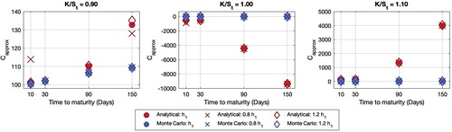
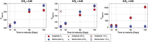
From Figure 1, the results of ATM and OTM cases from the proposed method appear unreasonable. In this simulation, the strike price K is set to be 900, 1000 and 1100 and the current stock price is 1000. However, the results of the ATM case is negative while those of the OTM case seem to be explosive when the time to maturity increases. This shows that the proposed method cannot estimate the option prices for both ATM and OTM cases. For the ITM case, the results from both methods show a similar pattern. Therefore, to deepen this study, more ITM cases, with $K/S_t=0.80,0.85$ and 0.95, are studied. From Figure 2, the results show that the behaviour of two option prices have the same trend when $K/S_t$=0.80 and 0.85. However, the analytical approximation prices are too high when $K/S_t$=0.95. Therefore, the results from these two methods seem to be uncorrelated when $K/S_t$ increases to 1.

Figure 2. Average of simulation results of an analytical approximation for call option prices: ‘ITM Cases’. Source: Created by the authors.

After getting the analytical option prices and analysing the behaviour of the approximated formula in comparison to the Monte Carlo approach, the impact of skewness and kurtosis is considered. In this point, the formulas are set into three cases as $${\text{Price}}_{nc}=C,{\text{Price}}_{sc}=C+{\kappa }_3{A}_3{\mathrm{}\text{and}\mathrm{}\text{Price}}_{\mathit{skc}}=C+{\kappa }_3{A}_3+({\kappa }_4-3)A_4,$$ where $C,{\kappa }_3,A_3,{\kappa }_4$ and A₄ are given in (5). Note that the Price_nc does not focus on the impact of both skewness and kurtosis while the Price_nc adjusted only the skewness is defined as the Price_sc. For the Price_skc, it is the formula in (5) that is the Price_nc adjusted by both skewness and kurtosis. One case of simulation result is shown in Figure 3. The results for other cases show the same trend.

Figure 3. Impact of skewness and kurtosis correspondence on call option prices. Source: Created by the authors.

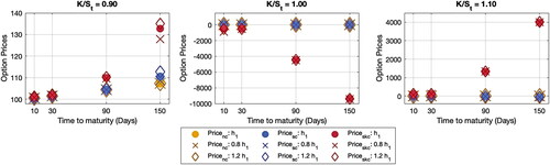
It can be seen in Figure 3 that the kurtosis affects the analytical approximation of option prices extremely because the ${\sigma }_{{\rho }_T}$ in (5) is so small. For the skewness, it does not provide a significant impact on the approximation.

5.2. Approximated option prices in real market

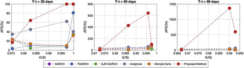
In this section, the analytical formula of option prices is applied to the real SET data. The accuracy of the analytical approximation is investigated by using four different measures in the case of ITM. In this study, the risk-free interest rate is set to be 1.99% per annum as the Thai government bond rate. The time to expiration (T – t) is considered to three cases: 30, 60 and 90 days. For other information, such as the asset prices at time t (S_t) and strike prices (K), the SET data are used as observation data. To approximate the option prices, we first compute the parameter values ${\alpha }_0,{\alpha }_1,{\beta }_1,{\gamma }_1$ and λ in (8). In this step, the maximum likelihood is used to estimate these appropriate parameters. The results of the new analytical approximation of call option prices are compared with the observation prices and prices obtained from the other methods such as the GARCH model, TGARCH model, GJR-GARCH model, analytical approximation via GARCH model and Monte Carlo simulation. The tools used to measure the accuracy of the results are correlation coefficient (CORR), mean absolute percentage Error (MAPE), root mean square error (RMSE) and maximum of absolute percentage error (MaxAPE). The formulas are given as follows: $$\begin{array}{c}\mathrm{}\text{CORR}=\frac{\sum _{i=1}^n(x_i-\overline{x})(y_i-\overline{y})}{\sqrt{\sum _{i=1}^n{(x_i-\overline{x})}^2\sum _{i=1}^n{(y_i-\overline{y})}^2}},\mathrm{}\text{MAPE}=\frac{100\%}{n}\times \sum _{i=1}^n\left|\frac{y_i-x_i}{x_i}\right|,\\ \text{RMSE}=\sqrt{\sum _{i=1}^n\frac{{(y_i-x_i)}^2}{n}}\mathrm{}\text{and}\mathrm{}\text{MaxAPE}=\underset{{}_{1\le i\le n}}{\max }(100\%\times |\frac{y_i-x_i}{x_i}\left|\right),\end{array}$$ where the y_i is the observed price, x_i is the estimated price, $\overline{y}$ is the mean of observed price, $\overline{x}$ is the mean of estimated price and n is the number of observations. The results in Table 3 reveal that, in the case that $K/S_t\le 0.95,$ the proposed method provides an excellent approximated price. From the CORR measure, the results from these six methods have a high positive relation to the observation prices. From MAPE, RMSE and MaxAPE, the proposed method gives more accuracy than the other approaches. This conclusion satisfies the result from the previous section. The results are shown in Table 3 and Figure 4.

Figure 4. CORR, MAPE, RMSE and MaxAPE of call option prices. Source: Created by the authors based on SET50 data.

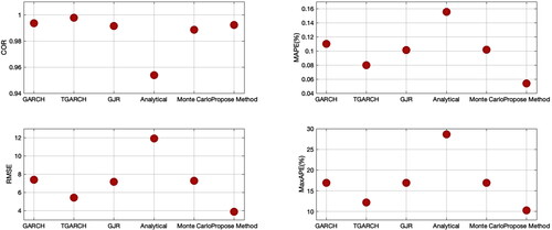
Table 3. The performance of option prices with $K/S_t\le 0.95.$

T–t	St	K	$K/S_t$	Observed	GARCH model (1995)	TGARCH model (2016)	GJR-GARCH model (1993)	Analytical approximation via GARCH (1999)	Monte Carlo simulation	Proposed method
30	1002.83	925	0.9224	77.1	80.9976	80.6944	80.6840	80.0163	81.2703	80.0169
		950	0.9473	53.6	57.3141	57.4602	57.7509	55.0754	59.1362	55.0768
	814.10	725	0.8906	87.0	91.6920	93.2941	91.3098	90.8136	90.5869	90.8142
		775	0.9520	44.8	50.4312	49.6412	46.7440	40.9319	44.7024	40.9375
	1025.18	925	0.9511	47.6	55.4279	52.6966	55.0622	59.1919	55.1542	52.4853
60	1002.57	950	0.9476	57.4	64.9077	64.4133	65.1244	73.2825	66.6853	57.0486
	1079.50	1000	0.9264	76.9	85.9039	84.1349	86.0368	90.3446	85.8393	84.2234
		1025	0.9495	56.3	63.9742	59.2604	63.8736	68.7463	63.8847	59.3415
90	1057.56	950	0.8983	111.1	120.4084	118.6975	120.2725	128.9308	119.4781	114.2647
	1085.81	1025	0.9440	64.5	75.4322	67.9778	75.3993	82.9388	75.4068	68.0643
				CORR	0.9935	0.9977	0.9915	0.9538	0.9886	0.9922
				MAPE	11.0139%	7.9727%	10.1307%	15.5802%	10.1672%	5.3720%
				RMSE	7.3924	5.4494	7.1523	11.9181	7.2855	3.8697
				MaxAPE	16.9492%	12.2183%	16.8981%	28.5873%	16.9097%	10.2632%

Source: Created by the authors based on SET50 data.

For the 11 ITM cases when $K/S_t$ approaches to 1, the results of the proposed method do not show a good performance, as can be seen in Figure 5.

Figure 5. Impact of $K/S_t$ correspondence on call option prices. Source: Created by the authors based on SET50 data.

However, after computing the 27 OTM cases with real-data option prices, the results of the proposed method reveal a poor performance. This method cannot capture the option prices. In most cases, the estimated prices are negative and then are set as 0.

6. Conclusion

An analytical approximation formula via the TGARCH model has been developed in this study. The formula is similar to the Black-Scholes formula, adjusted by the skewness and kurtosis of the cumulative asset return. The first four moments of the cumulative asset return are derived and computed by using the TGARCH model. The new proposed method generalises the Black-Scholes by reducing two assumptions: constant volatility and the lognormal distribution asset prices. After formulating the proposed method, both simulation and empirical results are studied. With these results, it is shown that in the case of ITM with $K/S_t\le 0.95,$ the behaviour of the analytical approximation via the TGARCH model does not significantly differ from the compared methods, such as GARCH, TGARCH, GJR-GARCH, analytical approximation via the GARCH model and Monte Carlo simulation. However, with regards to accuracy, the empirical results demonstrate that the analytical approximation via the TGARCH model is more accurate than the other methods. Furthermore, the analytical approximation via the TGARCH model required fewer assumptions than the Black-Scholes formula. Future research can be devoted to improving a new method with more general assumptions in the real market.

Acknowledgment

The authors would like to thank the referees for their careful reading and helpful comments.

Disclosure statement

No potential conflict of interest was reported by the authors.

Additional information

Funding

This research was supported by Petchra Pra Jom Klao Ph.D. Research Scholarship from King Mongkut’s University of Technology Thonburi (Grant No. 42/2559) and Theoretical and Computational Science Center (TaCS), Faculty of Science, KMUTT.

Appendix A:

Some general form of terms in the first four moments of cumulative asset return

This appendix is reserved for providing general forms of some expression terms in (7). We can derive these terms by

A.1 Some terms ending with $h_{i+j}^{\frac{1}{2}}$

$$E_0^Q\left[h_i^p{ϵ}_i^q{h}_{i+j}^{\frac{1}{2}}\right]={\alpha }_0\left(\frac{1-{\mu }_1^j}{1-{\mu }_1}\right)E_0^Q\left[h_i^p{ϵ}_i^q\right]+{\mu }_1^{j-1}{E}_0^Q\left[h_i^{p+\frac{1}{2}}{ϵ}_i^q{Y}_i\right].$$

If q = 0, we get $$E_0^Q\left[h_i^p{h}_{i+j}^{\frac{1}{2}}\right]={\alpha }_0\left(\frac{1-{\mu }_1^j}{1-{\mu }_1}\right)E_0^Q\left[h_i^p\right]+{\mu }_1^j{E}_0^Q\left[h_i^{p+\frac{1}{2}}\right].$$

If q = 1, we get $$E_0^Q\left[h_i^p{ϵ}_i{h}_{i+j}^{\frac{1}{2}}\right]={\mu }_1^{j-1}{\nu }_1{E}_0^Q\left[h_i^{p+\frac{1}{2}}\right].$$

If q = 2, we get $$E_0^Q\left[h_i^p{ϵ}_i^2{h}_{i+j}^{\frac{1}{2}}\right]={\alpha }_0\left(\frac{1-{\mu }_1^j}{1-{\mu }_1}\right)E_0^Q\left[h_i^p\right]+{\mu }_1^{j-1}{\zeta }_1{E}_0^Q\left[h_i^{p+\frac{1}{2}}\right].$$

A.2 Some terms ending with $h_{i+j}$

$$E_0^Q\left[h_i^p{ϵ}_i^q{h}_{i+j}\right]={\alpha }_0^2(\frac{1+{\mu }_1}{1-{\mu }_1}·\frac{1-{\mu }_2^j}{1-{\mu }_2}-2\frac{{\mu }_1}{1-{\mu }_1}·\frac{{\mu }_1^j-{\mu }_2^j}{{\mu }_1-{\mu }_2})E_0^Q\left[h_i^p{ϵ}_i^q\right]\backslash \backslash +2{\alpha }_0\left(\frac{{\mu }_1^j-{\mu }_2^j}{{\mu }_1-{\mu }_2}\right)E_0^Q\left[h_i^{p+\frac{1}{2}}{ϵ}_i^q{Y}_i\right]+{\mu }_2^{j-1}{E}_0^Q\left[h_i^{p+1}{ϵ}_i^q{Y}_i^2\right].$$

If q = 0, we get $$E_0^Q\left[h_i^p{h}_{i+j}\right]={\alpha }_0^2(\frac{1+{\mu }_1}{1-{\mu }_1}·\frac{1-{\mu }_2^j}{1-{\mu }_2}-2\frac{{\mu }_1}{1-{\mu }_1}·\frac{{\mu }_1^j-{\mu }_2^j}{{\mu }_1-{\mu }_2})E_0^Q\left[h_i^p\right]\backslash \backslash +2{\alpha }_0{\mu }_1\left(\frac{{\mu }_1^j-{\mu }_2^j}{{\mu }_1-{\mu }_2}\right)E_0^Q\left[h_i^{p+\frac{1}{2}}\right]+{\mu }_2^j{E}_0^Q\left[h_i^{p+1}\right].$$

If q = 1, we get $$E_0^Q\left[h_i^p{ϵ}_i{h}_{i+j}\right]=2{\alpha }_0{\nu }_1\left(\frac{{\mu }_1^j-{\mu }_2^j}{{\mu }_1-{\mu }_2}\right)E_0^Q\left[h_i^{p+\frac{1}{2}}\right]+{\mu }_2^{j-1}{\nu }_2{E}_0^Q\left[h_i^{p+1}\right].$$

If q = 2, we get $$E_0^Q\left[h_i^p{ϵ}_i^2{h}_{i+j}\right]={\alpha }_0^2(\frac{1+{\mu }_1}{1-{\mu }_1}·\frac{1-{\mu }_2^j}{1-{\mu }_2}-2\frac{{\mu }_1}{1-{\mu }_1}·\frac{{\mu }_1^j-{\mu }_2^j}{{\mu }_1-{\mu }_2})E_0^Q\left[h_i^p\right]\backslash \backslash +2{\alpha }_0{\zeta }_1\left(\frac{{\mu }_1^j-{\mu }_2^j}{{\mu }_1-{\mu }_2}\right)E_0^Q\left[h_i^{p+\frac{1}{2}}\right]+{\mu }_2^{j-1}{\zeta }_2{E}_0^Q\left[h_i^{p+1}\right].$$

If q = 3, we get $$E_0^Q\left[h_i^p{ϵ}_i^3{h}_{i+j}\right]=2{\alpha }_0{\eta }_1\left(\frac{{\mu }_1^j-{\mu }_2^j}{{\mu }_1-{\mu }_2}\right)E_0^Q\left[h_i^{p+\frac{1}{2}}\right]+{\mu }_2^{j-1}{\eta }_2{E}_0^Q\left[h_i^{p+1}\right].$$

A.3 Some terms ending with $h_{i+j+k}^{\frac{1}{2}}$

$$E_0^Q\left[h_i^p{ϵ}_i^q{h}_{i+j}^r{ϵ}_{i+j}^s{h}_{i+j+k}^{\frac{1}{2}}\right]={\alpha }_0\left(\frac{1-{\mu }_1^k}{1-{\mu }_1}\right)E_0^Q\left[h_i^p{ϵ}_i^q{h}_{i+j}^r{ϵ}_{i+j}^s\right]+{\mu }_1^{k-1}{E}_0^Q\left[h_i^p{ϵ}_i^q{h}_{i+j}^{r+\frac{1}{2}}{ϵ}_{i+j}^s{Y}_{i+j}\right].$$

If s = 0, we get $$E_0^Q\left[h_i^p{ϵ}_i^q{h}_{i+j}^r{h}_{i+j+k}^{\frac{1}{2}}\right]={\alpha }_0\left(\frac{1-{\mu }_1^k}{1-{\mu }_1}\right)E_0^Q\left[h_i^p{ϵ}_i^q{h}_{i+j}^r\right]+{\mu }_1^k{E}_0^Q\left[h_i^p{ϵ}_i^q{h}_{i+j}^{r+\frac{1}{2}}\right].$$

If s = 1, we get $$E_0^Q\left[h_i^p{ϵ}_i^q{h}_{i+j}^r{ϵ}_{i+j}{h}_{i+j+k}^{\frac{1}{2}}\right]={\mu }_1^{k-1}{\nu }_1{E}_0^Q\left[h_i^p{ϵ}_i^q{h}_{i+j}^{r+\frac{1}{2}}\right].$$

A.4 Some terms ending with $h_{i+j+k}$

$$\begin{array}{c}{E}_0^Q\left[h_i^p{ϵ}_i^q{h}_{i+j}^r{ϵ}_{i+j}^s{h}_{i+j+k}\right]={\alpha }_0^2(\frac{1+{\mu }_1}{1-{\mu }_1}·\frac{1-{\mu }_2^k}{1-{\mu }_2}-2\frac{{\mu }_1}{1-{\mu }_1}·\frac{{\mu }_1^k-{\mu }_2^k}{{\mu }_1-{\mu }_2})E_0^Q\left[h_i^p{ϵ}_i^q{h}_{i+j}^r{ϵ}_{i+j}^s\right]\\ +2{\alpha }_0\left(\frac{{\mu }_1^k-{\mu }_2^k}{{\mu }_1-{\mu }_2}\right)E_0^Q\left[h_i^p{ϵ}_i^q{h}_{i+j}^{r+\frac{1}{2}}{ϵ}_{i+j}^s{Y}_{i+j}\right]\\ +{\mu }_2^{k-1}{E}_0^Q\left[h_i^p{ϵ}_i^q{h}_{i+j}^{r+1}{ϵ}_{i+j}^s{Y}_{i+j}^2\right].\end{array}$$

If s = 0, we get $$\begin{array}{c}{E}_0^Q\left[h_i^p{ϵ}_i^q{h}_{i+j}^r{h}_{i+j+k}\right]={\alpha }_0^2(\frac{1+{\mu }_1}{1-{\mu }_1}·\frac{1-{\mu }_2^k}{1-{\mu }_2}-2\frac{{\mu }_1}{1-{\mu }_1}·\frac{{\mu }_1^k-{\mu }_2^k}{{\mu }_1-{\mu }_2})E_0^Q\left[h_i^p{ϵ}_i^q{h}_{i+j}^r\right]\\ +2{\alpha }_0{\mu }_1\left(\frac{{\mu }_1^k-{\mu }_2^k}{{\mu }_1-{\mu }_2}\right)E_0^Q\left[h_i^p{ϵ}_i^q{h}_{i+j}^{r+\frac{1}{2}}\right]+{\mu }_2^k{E}_0^Q\left[h_i^p{ϵ}_i^q{h}_{i+j}^{r+1}\right].\end{array}$$

If s = 1, we get $$E_0^Q\left[h_i^p{ϵ}_i^q{h}_{i+j}^r{ϵ}_{i+j}{h}_{i+j+k}\right]=2{\alpha }_0{\nu }_1\left(\frac{{\mu }_1^k-{\mu }_2^k}{{\mu }_1-{\mu }_2}\right)E_0^Q\left[h_i^p{ϵ}_i^q{h}_{i+j}^{r+\frac{1}{2}}\right]+{\mu }_2^{k-1}{\nu }_2{E}_0^Q\left[h_i^p{ϵ}_i^q{h}_{i+j}^{r+1}\right].$$

If s = 2, we get $$\begin{array}{c}{E}_0^Q\left[h_i^p{ϵ}_i^q{h}_{i+j}^r{ϵ}_{i+j}^s{h}_{i+j+k}\right]={\alpha }_0^2(\frac{1+{\mu }_1}{1-{\mu }_1}·\frac{1-{\mu }_2^k}{1-{\mu }_2}-2\frac{{\mu }_1}{1-{\mu }_1}·\frac{{\mu }_1^k-{\mu }_2^k}{{\mu }_1-{\mu }_2})E_0^Q\left[h_i^p{ϵ}_i^q{h}_{i+j}^r\right]\\ +2{\alpha }_0{\zeta }_1\left(\frac{{\mu }_1^k-{\mu }_2^k}{{\mu }_1-{\mu }_2}\right)E_0^Q\left[h_i^p{ϵ}_i^q{h}_{i+j}^{r+\frac{1}{2}}\right]+{\mu }_2^{k-1}{\zeta }_2{E}_0^Q\left[h_i^p{ϵ}_i^q{h}_{i+j}^{r+1}\right].\end{array}$$

A.5 Some terms ending with $h_{i+j+k+m}$

$$\begin{array}{c}{E}_0^Q\left[h_i^p{ϵ}_i^q{h}_{i+j}^r{ϵ}_{i+j}^s{h}_{i+j+k}^t{ϵ}_{i+j+k}^u{h}_{i+j+k+m}\right]={\alpha }_0^2(\frac{1+{\mu }_1}{1-{\mu }_1}·\frac{1-{\mu }_2^m}{1-{\mu }_2}-2\frac{{\mu }_1}{1-{\mu }_1}·\frac{{\mu }_1^m-{\mu }_2^m}{{\mu }_1-{\mu }_2})E_0^Q\left[h_i^p{ϵ}_i^q{h}_{i+j}^r{ϵ}_{i+j}^s{h}_{i+j+k}^t{ϵ}_{i+j+k}^u\right]\\ +2{\alpha }_0\left(\frac{{\mu }_1^m-{\mu }_2^m}{{\mu }_1-{\mu }_2}\right)E_0^Q\left[h_i^p{ϵ}_i^q{h}_{i+j}^r{ϵ}_{i+j}^s{h}_{i+j+k}^{t+\frac{1}{2}}{ϵ}_{i+j+k}^u{Y}_{i+j+k}\right]\\ +{\mu }_2^{m-1}{E}_0^Q\left[h_i^p{ϵ}_i^q{h}_{i+j}^r{ϵ}_{i+j}^s{h}_{i+j+k}^{t+1}{ϵ}_{i+j+k}^u{Y}_{i+j+k}^2\right].\end{array}$$

If u = 0, we get $$\begin{array}{c}{E}_0^Q\left[h_i^p{ϵ}_i^q{h}_{i+j}^r{ϵ}_{i+j}^s{h}_{i+j+k}^t{h}_{i+j+k+m}\right]={\alpha }_0^2(\frac{1+{\mu }_1}{1-{\mu }_1}·\frac{1-{\mu }_2^m}{1-{\mu }_2}-2\frac{{\mu }_1}{1-{\mu }_1}·\frac{{\mu }_1^m-{\mu }_2^m}{{\mu }_1-{\mu }_2})E_0^Q\left[h_i^p{ϵ}_i^q{h}_{i+j}^r{ϵ}_{i+j}^s{h}_{i+j+k}^t\right]\\ +2{\alpha }_0{\mu }_1\left(\frac{{\mu }_1^m-{\mu }_2^m}{{\mu }_1-{\mu }_2}\right)E_0^Q\left[h_i^p{ϵ}_i^q{h}_{i+j}^r{ϵ}_{i+j}^s{h}_{i+j+k}^{t+\frac{1}{2}}\right]\\ +{\mu }_2^m{E}_0^Q\left[h_i^p{ϵ}_i^q{h}_{i+j}^r{ϵ}_{i+j}^s{h}_{i+j+k}^{t+1}\right].\end{array}$$

If u = 1, we get $$\begin{array}{c}{E}_0^Q\left[h_i^p{ϵ}_i^q{h}_{i+j}^r{ϵ}_{i+j}^s{h}_{i+j+k}^t{ϵ}_{i+j+k}{h}_{i+j+k+m}\right]=2{\alpha }_0{\nu }_1\left(\frac{{\mu }_1^m-{\mu }_2^m}{{\mu }_1-{\mu }_2}\right)E_0^Q\left[h_i^p{ϵ}_i^q{h}_{i+j}^r{ϵ}_{i+j}^s{h}_{i+j+k}^{t+\frac{1}{2}}\right]\\ +{\mu }_2^{m-1}{\nu }_2{E}_0^Q\left[h_i^p{ϵ}_i^q{h}_{i+j}^r{ϵ}_{i+j}^s{h}_{i+j+k}^{t+1}\right].\end{array}$$

A.6 Some terms ending with $h_{i+j}^{\frac{3}{2}}$

$$\begin{array}{c}{E}_0^Q\left[h_i^p{ϵ}_i^q{h}_{i+j}^{\frac{3}{2}}\right]={\alpha }_0^3[\frac{1-{\mu }_3^j}{1-{\mu }_3}+3(\frac{{\mu }_2}{1-{\mu }_2}·\frac{1-{\mu }_3^j}{1-{\mu }_3}-\frac{{\mu }_2}{1-{\mu }_2}·\frac{{\mu }_2^j-{\mu }_3^j}{{\mu }_2-{\mu }_3})\\ +3(\frac{{\mu }_1}{1-{\mu }_1}·\frac{1-{\mu }_3^j}{1-{\mu }_3}-\frac{{\mu }_1}{1-{\mu }_1}·\frac{{\mu }_1^j-{\mu }_3^j}{{\mu }_1-{\mu }_3})\\ +6(\frac{{\mu }_1}{1-{\mu }_1}·\frac{{\mu }_2}{1-{\mu }_2}·\frac{1-{\mu }_3^j}{1-{\mu }_3}-\frac{{\mu }_1}{1-{\mu }_1}·\frac{{\mu }_2}{1-{\mu }_2}·\frac{{\mu }_2^j-{\mu }_3^j}{{\mu }_2-{\mu }_3}\\ -\frac{{\mu }_1}{1-{\mu }_1}·\frac{{\mu }_2}{{\mu }_1-{\mu }_2}·\frac{{\mu }_1^j-{\mu }_3^j}{{\mu }_1-{\mu }_3}+\frac{{\mu }_1}{1-{\mu }_1}·\frac{{\mu }_2}{{\mu }_1-{\mu }_2}·\frac{{\mu }_2^j-{\mu }_3^j}{{\mu }_2-{\mu }_3}\left)\right]E_0^Q\left[h_i^p{ϵ}_i^q\right]\\ +3{\alpha }_0^2[\frac{{\mu }_1^j-{\mu }_3^j}{{\mu }_1-{\mu }_3}+2(\frac{{\mu }_2}{{\mu }_1-{\mu }_2}·\frac{{\mu }_1^j-{\mu }_3^j}{{\mu }_1-{\mu }_3}-\frac{{\mu }_2}{{\mu }_1-{\mu }_2}·\frac{{\mu }_2^j-{\mu }_3^j}{{\mu }_2-{\mu }_3}\left)\right]E_0^Q\left[h_i^{p+\frac{1}{2}}{ϵ}_i^q{Y}_i\right]\\ +3{\alpha }_0\left(\frac{{\mu }_2^j-{\mu }_3^j}{{\mu }_2-{\mu }_3}\right)E_0^Q\left[h_i^{p+1}{ϵ}_i^q{Y}_i^2\right]+{\mu }_3^{j-1}{E}_0^Q\left[h_i^{p+\frac{3}{2}}{ϵ}_i^q{Y}_i^3\right].\end{array}$$

If q = 0, we get $$\begin{array}{c}{E}_0^Q\left[h_i^p{h}_{i+j}^{\frac{3}{2}}\right]={\alpha }_0^3[\frac{1-{\mu }_3^j}{1-{\mu }_3}+3(\frac{{\mu }_2}{1-{\mu }_2}·\frac{1-{\mu }_3^j}{1-{\mu }_3}-\frac{{\mu }_2}{1-{\mu }_2}·\frac{{\mu }_2^j-{\mu }_3^j}{{\mu }_2-{\mu }_3})\\ +3(\frac{{\mu }_1}{1-{\mu }_1}·\frac{1-{\mu }_3^j}{1-{\mu }_3}-\frac{{\mu }_1}{1-{\mu }_1}·\frac{{\mu }_1^j-{\mu }_3^j}{{\mu }_1-{\mu }_3})\\ +6(\frac{{\mu }_1}{1-{\mu }_1}·\frac{{\mu }_2}{1-{\mu }_2}·\frac{1-{\mu }_3^j}{1-{\mu }_3}-\frac{{\mu }_1}{1-{\mu }_1}·\frac{{\mu }_2}{1-{\mu }_2}·\frac{{\mu }_2^j-{\mu }_3^j}{{\mu }_2-{\mu }_3}\\ -\frac{{\mu }_1}{1-{\mu }_1}·\frac{{\mu }_2}{{\mu }_1-{\mu }_2}·\frac{{\mu }_1^j-{\mu }_3^j}{{\mu }_1-{\mu }_3}+\frac{{\mu }_1}{1-{\mu }_1}·\frac{{\mu }_2}{{\mu }_1-{\mu }_2}·\frac{{\mu }_2^j-{\mu }_3^j}{{\mu }_2-{\mu }_3}\left)\right]E_0^Q\left[h_i^p\right]\\ +3{\alpha }_0^2{\mu }_1[\frac{{\mu }_1^j-{\mu }_3^j}{{\mu }_1-{\mu }_3}+2(\frac{{\mu }_2}{{\mu }_1-{\mu }_2}·\frac{{\mu }_1^j-{\mu }_3^j}{{\mu }_1-{\mu }_3}-\frac{{\mu }_2}{{\mu }_1-{\mu }_2}·\frac{{\mu }_2^j-{\mu }_3^j}{{\mu }_2-{\mu }_3}\left)\right]E_0^Q\left[h_i^{p+\frac{1}{2}}\right]\\ +3{\alpha }_0{\mu }_2\left(\frac{{\mu }_2^j-{\mu }_3^j}{{\mu }_2-{\mu }_3}\right)E_0^Q\left[h_i^{p+1}\right]+{\mu }_3^j{E}_0^Q\left[h_i^{p+\frac{3}{2}}\right].\end{array}$$

If q = 1, we get $$\begin{array}{c}{E}_0^Q\left[h_i^pϵh_{i+j}^{\frac{3}{2}}\right]=3{\alpha }_0^2{\nu }_1[\frac{{\mu }_1^j-{\mu }_3^j}{{\mu }_1-{\mu }_3}+2(\frac{{\mu }_2}{{\mu }_1-{\mu }_2}·\frac{{\mu }_1^j-{\mu }_3^j}{{\mu }_1-{\mu }_3}-\frac{{\mu }_2}{{\mu }_1-{\mu }_2}·\frac{{\mu }_2^j-{\mu }_3^j}{{\mu }_2-{\mu }_3}\left)\right]E_0^Q\left[h_i^{p+\frac{1}{2}}\right]\\ +3{\alpha }_0{\nu }_2\left(\frac{{\mu }_2^j-{\mu }_3^j}{{\mu }_2-{\mu }_3}\right)E_0^Q\left[h_i^{p+1}\right]+{\mu }_3^{j-1}{\nu }_3{E}_0^Q\left[h_i^{p+\frac{3}{2}}\right].\end{array}$$

If q = 2, we get $$\begin{array}{c}{E}_0^Q\left[h_i^p{ϵ}^2{h}_{i+j}^{\frac{3}{2}}\right]={\alpha }_0^3[\frac{1-{\mu }_3^j}{1-{\mu }_3}+3(\frac{{\mu }_2}{1-{\mu }_2}·\frac{1-{\mu }_3^j}{1-{\mu }_3}-\frac{{\mu }_2}{1-{\mu }_2}·\frac{{\mu }_2^j-{\mu }_3^j}{{\mu }_2-{\mu }_3})\\ +3(\frac{{\mu }_1}{1-{\mu }_1}·\frac{1-{\mu }_3^j}{1-{\mu }_3}-\frac{{\mu }_1}{1-{\mu }_1}·\frac{{\mu }_1^j-{\mu }_3^j}{{\mu }_1-{\mu }_3})\\ +6(\frac{{\mu }_1}{1-{\mu }_1}·\frac{{\mu }_2}{1-{\mu }_2}·\frac{1-{\mu }_3^j}{1-{\mu }_3}-\frac{{\mu }_1}{1-{\mu }_1}·\frac{{\mu }_2}{1-{\mu }_2}·\frac{{\mu }_2^j-{\mu }_3^j}{{\mu }_2-{\mu }_3}\\ -\frac{{\mu }_1}{1-{\mu }_1}·\frac{{\mu }_2}{{\mu }_1-{\mu }_2}·\frac{{\mu }_1^j-{\mu }_3^j}{{\mu }_1-{\mu }_3}+\frac{{\mu }_1}{1-{\mu }_1}·\frac{{\mu }_2}{{\mu }_1-{\mu }_2}·\frac{{\mu }_2^j-{\mu }_3^j}{{\mu }_2-{\mu }_3}\left)\right]E_0^Q\left[h_i^p\right]\\ +3{\alpha }_0^2{\zeta }_1[\frac{{\mu }_1^j-{\mu }_3^j}{{\mu }_1-{\mu }_3}+2(\frac{{\mu }_2}{{\mu }_1-{\mu }_2}·\frac{{\mu }_1^j-{\mu }_3^j}{{\mu }_1-{\mu }_3}-\frac{{\mu }_2}{{\mu }_1-{\mu }_2}·\frac{{\mu }_2^j-{\mu }_3^j}{{\mu }_2-{\mu }_3}\left)\right]E_0^Q\left[h_i^{p+\frac{1}{2}}\right]\\ +3{\alpha }_0{\zeta }_2\left(\frac{{\mu }_2^j-{\mu }_3^j}{{\mu }_2-{\mu }_3}\right)E_0^Q\left[h_i^{p+1}\right]+{\mu }_3^{j-1}{\zeta }_3{E}_0^Q\left[h_i^{p+\frac{3}{2}}\right].\end{array}$$

A.7 Some terms ending with $h_{i+j+k}^{\frac{3}{2}}$

$$\begin{array}{c}{E}_0^Q\left[h_i^p{ϵ}_i^q{h}_{i+j}^r{ϵ}_{i+j}^s{h}_{i+j+k}^{\frac{3}{2}}\right]={\alpha }_0^3[\frac{1-{\mu }_3^k}{1-{\mu }_3}+3(\frac{{\mu }_2}{1-{\mu }_2}·\frac{1-{\mu }_3^k}{1-{\mu }_3}-\frac{{\mu }_2}{1-{\mu }_2}·\frac{{\mu }_2^k-{\mu }_3^k}{{\mu }_2-{\mu }_3})\\ +3(\frac{{\mu }_1}{1-{\mu }_1}·\frac{1-{\mu }_3^k}{1-{\mu }_3}-\frac{{\mu }_1}{1-{\mu }_1}·\frac{{\mu }_1^k-{\mu }_3^k}{{\mu }_1-{\mu }_3})\\ +6(\frac{{\mu }_1}{1-{\mu }_1}·\frac{{\mu }_2}{1-{\mu }_2}·\frac{1-{\mu }_3^k}{1-{\mu }_3}-\frac{{\mu }_1}{1-{\mu }_1}·\frac{{\mu }_2}{1-{\mu }_2}·\frac{{\mu }_2^k-{\mu }_3^k}{{\mu }_2-{\mu }_3}\\ -\frac{{\mu }_1}{1-{\mu }_1}·\frac{{\mu }_2}{{\mu }_1-{\mu }_2}·\frac{{\mu }_1^k-{\mu }_3^k}{{\mu }_1-{\mu }_3}+\frac{{\mu }_1}{1-{\mu }_1}·\frac{{\mu }_2}{{\mu }_1-{\mu }_2}·\frac{{\mu }_2^k-{\mu }_3^k}{{\mu }_2-{\mu }_3}\left)\right]E_0^Q\left[h_i^p{ϵ}_i^q{h}_{i+j}^r{ϵ}_{i+j}^s\right]\\ +3{\alpha }_0^2[\frac{{\mu }_1^k-{\mu }_3^k}{{\mu }_1-{\mu }_3}+2(\frac{{\mu }_2}{{\mu }_1-{\mu }_2}·\frac{{\mu }_1^k-{\mu }_3^k}{{\mu }_1-{\mu }_3}-\frac{{\mu }_2}{{\mu }_1-{\mu }_2}·\frac{{\mu }_2^k-{\mu }_3^k}{{\mu }_2-{\mu }_3}\left)\right]E_0^Q\left[h_i^p{ϵ}_i^q{h}_{i+j}^{r+\frac{1}{2}}{ϵ}_{i+j}^s{Y}_{i+j}\right]\\ +3{\alpha }_0\left(\frac{{\mu }_2^k-{\mu }_3^k}{{\mu }_2-{\mu }_3}\right)E_0^Q\left[h_i^{p1}{ϵ}_i^q{h}_{i+j}^{r+1}{ϵ}_{i+j}^s{Y}_{i+j}^2\right]+{\mu }_3^{j-1}{E}_0^Q\left[h_i^p{ϵ}_i^q{h}_{i+j}^{r+\frac{3}{2}}{ϵ}_{i+j}^s{Y}_{i+j}^3\right].\end{array}$$

If s = 0, we get $$\begin{array}{c}{E}_0^Q\left[h_i^p{ϵ}_i^q{h}_{i+j}^r{h}_{i+j+k}^{\frac{3}{2}}\right]={\alpha }_0^3[\frac{1-{\mu }_3^k}{1-{\mu }_3}+3(\frac{{\mu }_2}{1-{\mu }_2}·\frac{1-{\mu }_3^k}{1-{\mu }_3}-\frac{{\mu }_2}{1-{\mu }_2}·\frac{{\mu }_2^k-{\mu }_3^k}{{\mu }_2-{\mu }_3})+3(\frac{{\mu }_1}{1-{\mu }_1}·\frac{1-{\mu }_3^k}{1-{\mu }_3}-\frac{{\mu }_1}{1-{\mu }_1}·\frac{{\mu }_1^k-{\mu }_3^k}{{\mu }_1-{\mu }_3})\\ +6(\frac{{\mu }_1}{1-{\mu }_1}·\frac{{\mu }_2}{1-{\mu }_2}·\frac{1-{\mu }_3^k}{1-{\mu }_3}-\frac{{\mu }_1}{1-{\mu }_1}·\frac{{\mu }_2}{1-{\mu }_2}·\frac{{\mu }_2^k-{\mu }_3^k}{{\mu }_2-{\mu }_3}\\ -\frac{{\mu }_1}{1-{\mu }_1}·\frac{{\mu }_2}{{\mu }_1-{\mu }_2}·\frac{{\mu }_1^k-{\mu }_3^k}{{\mu }_1-{\mu }_3}+\frac{{\mu }_1}{1-{\mu }_1}·\frac{{\mu }_2}{{\mu }_1-{\mu }_2}·\frac{{\mu }_2^k-{\mu }_3^k}{{\mu }_2-{\mu }_3}\left)\right]E_0^Q\left[h_i^p{ϵ}_i^q{h}_{i+j}^r\right]\\ +3{\alpha }_0^2{\mu }_1[\frac{{\mu }_1^k-{\mu }_3^k}{{\mu }_1-{\mu }_3}+2(\frac{{\mu }_2}{{\mu }_1-{\mu }_2}·\frac{{\mu }_1^k-{\mu }_3^k}{{\mu }_1-{\mu }_3}-\frac{{\mu }_2}{{\mu }_1-{\mu }_2}·\frac{{\mu }_2^k-{\mu }_3^k}{{\mu }_2-{\mu }_3}\left)\right]E_0^Q\left[h_i^p{ϵ}_i^q{h}_{i+j}^{r+\frac{1}{2}}\right]\\ +3{\alpha }_0{\mu }_2\left(\frac{{\mu }_2^k-{\mu }_3^k}{{\mu }_2-{\mu }_3}\right)E_0^Q\left[h_i^{p1}{ϵ}_i^q{h}_{i+j}^{r+1}\right]+{\mu }_3^j{E}_0^Q\left[h_i^p{ϵ}_i^q{h}_{i+j}^{r+\frac{3}{2}}\right].\end{array}$$

If s = 1, we get $$\begin{array}{c}{E}_0^Q\left[h_i^p{ϵ}_i^q{h}_{i+j}^r{ϵ}_{i+j}{h}_{i+j+k}^{\frac{3}{2}}\right]=3{\alpha }_0^2{\nu }_1[\frac{{\mu }_1^k-{\mu }_3^k}{{\mu }_1-{\mu }_3}+2(\frac{{\mu }_2}{{\mu }_1-{\mu }_2}·\frac{{\mu }_1^k-{\mu }_3^k}{{\mu }_1-{\mu }_3}-\frac{{\mu }_2}{{\mu }_1-{\mu }_2}·\frac{{\mu }_2^k-{\mu }_3^k}{{\mu }_2-{\mu }_3}\left)\right]E_0^Q\left[h_i^p{ϵ}_i^q{h}_{i+j}^{r+\frac{1}{2}}\right]\\ +3{\alpha }_0{\nu }_2\left(\frac{{\mu }_2^k-{\mu }_3^k}{{\mu }_2-{\mu }_3}\right)E_0^Q\left[h_i^{p1}{ϵ}_i^q{h}_{i+j}^{r+1}\right]+{\mu }_3^{j-1}{\nu }_3{E}_0^Q\left[h_i^p{ϵ}_i^q{h}_{i+j}^{r+\frac{3}{2}}\right].\end{array}$$

Appendix B:

Proof of Proposition 4.1

Proof.

It can be derived by using an integration by parts that $$\begin{array}{c}{E}_0^Q[{ϵ}_t^{n}I({ϵ}_t\ge \lambda )]=\frac{e^{-\frac{{\lambda }^2}{2}}}{\sqrt{2\pi }}\left\{{\lambda }^{n-1}\right[1+(n-1){\lambda }^{-2}]+(n-1)(n-3)\},n=1,3,5,\\ E_0^Q[{ϵ}_t^{n}I({ϵ}_t\ge \lambda )]=\frac{\lambda e^{-\frac{{\lambda }^2}{2}}}{\sqrt{2\pi }}[{\lambda }^{n-2}+(n-1)]+(n-1)[1-\Phi (\lambda )],n=2,4.\end{array}$$

With this facts and fact that $$E_0^Q\left[{ϵ}_t^n\right|{ϵ}_t-\lambda \left|\right]=E_0^Q\left[{ϵ}_t^n\right|{ϵ}_t-\lambda |I({ϵ}_t\ge \lambda )]+E_0^Q\left[{ϵ}_t^n\right|{ϵ}_t-\lambda |I({ϵ}_t<\lambda )],n=1,2,3,4,$$

where I is an indicator function, we have $$\begin{array}{c}{E}_0^Q\left[\right|{ϵ}_t-\lambda \left|\right]=\frac{2e^{-\frac{{\lambda }^2}{2}}}{\sqrt{2\pi }}-\lambda [1-2\Phi (\lambda )],E_0^Q\left[{ϵ}_t\right|{ϵ}_t-\lambda \left|\right]=1-2\Phi (\lambda ),\\ E_0^Q\left[{ϵ}_t^2\right|{ϵ}_t-\lambda \left|\right]=\frac{4e^{-\frac{{\lambda }^2}{2}}}{\sqrt{2\pi }}-\lambda [1-2\Phi (\lambda )],E_0^Q\left[{ϵ}_t^3\right|{ϵ}_t-\lambda \left|\right]=\frac{2\lambda e^{-\frac{{\lambda }^2}{2}}}{\sqrt{2\pi }}+3[1-2\Phi (\lambda )]\mathrm{}\text{and}\\ E_0^Q\left[{ϵ}_t^4\right|{ϵ}_t-\lambda \left|\right]=\frac{2e^{-\frac{{\lambda }^2}{2}}}{\sqrt{2\pi }}({\lambda }^2-8)-3\lambda [1-2\Phi (\lambda )].\end{array}$$

The proof can be completed by applying the above equations, the fact that $E_0^Q[{ϵ}_t^n]=0$ when n is odd, $E_0^Q[{ϵ}_t^k]=k-1$ when k is even to the equations: $$\begin{array}{c}{\mu }_1=E_0^Q\left[Y_t\right]={\beta }_1+{\alpha }_1{\gamma }_1\lambda +{\alpha }_1{E}_0^Q\left[\right|{ϵ}_t-\lambda \left|\right],\\ {\mu }_2=E_0^Q\left[Y_t^2\right]={\beta }_1({\beta }_1+2{\alpha }_1{\gamma }_1\lambda )+{\alpha }_1^2(1+{\lambda }^2)(1+{\gamma }_1^2)+2{\alpha }_1({\beta }_1+2{\gamma }_1\lambda )E_0^Q\left[\right|{ϵ}_t-\lambda \left|\right]\\ +2{\alpha }_1^2{\gamma }_1{E}_0^Q\left[{ϵ}_t\right|{ϵ}_t-\lambda \left|\right],\\ {\mu }_3=E_0^Q\left[Y_t^3\right]={\beta }_1^2({\beta }_1+3{\alpha }_1{\gamma }_1\lambda )+{\alpha }_1[{\alpha }_1^2{\gamma }_1\lambda (3+{\lambda }^2)(3+{\gamma }_1^2)+3{\alpha }_1{\beta }_1(1+{\lambda }^2)(1+{\gamma }_1^2)]\\ +[{\alpha }_1^3{\lambda }^2(1+3{\gamma }_1^2)+3{\alpha }_1{\beta }_1({\beta }_1+2{\alpha }_1{\gamma }_1)]E_0^Q\left[\right|{ϵ}_t-\lambda \left|\right]\\ -2{\alpha }_1^2[{\alpha }_1\lambda +3{\gamma }_1({\beta }_1+{\alpha }_1{\gamma }_1\lambda )]E_0^Q\left[{ϵ}_t\right|{ϵ}_t-\lambda \left|\right]+{\alpha }_1^3(1+3{\gamma }_1^2)E_0^Q\left[{ϵ}_t^2\right|{ϵ}_t-\lambda \left|\right],\\ {\nu }_1=E_0^Q\left[{ϵ}_t{Y}_t\right]={\alpha }_1{E}_0^Q\left[{ϵ}_t\right|{ϵ}_t-\lambda \left|\right]-{\alpha }_1{\gamma }_1,\\ {\nu }_2=E_0^Q\left[{ϵ}_t{Y}_t^2\right]=-2{\alpha }_1[{\alpha }_1\lambda (1+{\gamma }_1^2)+{\gamma }_1{\beta }_1]-2{\alpha }_1({\beta }_1+2{\alpha }_1{\gamma }_1\lambda )E_0^Q\left[{ϵ}_t\right|{ϵ}_t-\lambda \left|\right]-2{\alpha }_1^2{\gamma }_1{E}_0^Q\left[{ϵ}_t^2\right|{ϵ}_t-\lambda \left|\right],\\ {\nu }_3=E_0^Q\left[{ϵ}_t{Y}_t^3\right]=-3{\alpha }_1[{\alpha }_1^2{\gamma }_1(1+{\lambda }^2)(3+{\gamma }_1^2)+{\beta }_1({\gamma }_1{\beta }_1+2{\alpha }_1\lambda (1+{\gamma }_1^2))]\\ +{\alpha }_1[{\alpha }_1^2{\lambda }^2(1+3{\gamma }_1^2)+3{\beta }_1({\beta }_1+2{\alpha }_1{\gamma }_1\lambda )]E_0^Q\left[{ϵ}_t\right|{ϵ}_t-\lambda \left|\right]-2{\alpha }_1^2[{\alpha }_1\lambda (1+3{\gamma }_1^2)\\ +3{\gamma }_1{\beta }_1\left]E_0^Q\right[{ϵ}_t^2|{ϵ}_t-\lambda |]+{\alpha }_1^3(1+3{\gamma }_1^2)E_0^Q[{ϵ}_t^3|{ϵ}_t-\lambda |],\\ {\zeta }_1=E_0^Q\left[{ϵ}_t^2{Y}_t\right]={\beta }_1+{\alpha }_1{\gamma }_1\lambda +{\alpha }_1{E}_0^Q\left[{ϵ}_t^2\right|{ϵ}_t-\lambda \left|\right],\\ {\zeta }_2=E_0^Q\left[{ϵ}_t^2{Y}_t^2\right]={\alpha }_1^2(3+{\lambda }^2)(1+{\gamma }_1^2)+{\beta }_1({\beta }_1+2{\alpha }_1{\gamma }_1\lambda )+2{\alpha }_1({\beta }_1+{\alpha }_1{\gamma }_1\lambda )E_0^Q\left[{ϵ}_t^2\right|{ϵ}_t-\lambda \left|\right]\\ -2{\alpha }_1^2{\gamma }_1{E}_0^Q\left[{ϵ}_t^3\right|{ϵ}_t-\lambda \left|\right],\\ {\zeta }_3=E_0^Q\left[{ϵ}_t^2{Y}_t^3\right]={\beta }_1^2({\beta }_1+3{\alpha }_1{\gamma }_1\lambda )+{\alpha }_1^2[{\alpha }_1{\gamma }_1\lambda ({\lambda }^2+9)(3+{\gamma }_1^2)+3{\beta }_1(3+\lambda )(1+{\gamma }_1^2)]\\ +[{\alpha }_1^3{\lambda }^2(1+3{\gamma }_1^2)+3{\alpha }_1{\beta }_1({\beta }_1+2{\alpha }_1{\gamma }_1\lambda )]E_0^Q\left[{ϵ}_t^2\right|{ϵ}_t-\lambda \left|\right]\\ -2{\alpha }_1^2[{\alpha }_1\lambda (1+3{\gamma }_1^2)+3{\gamma }_1{\beta }_1]E_0^Q\left[{ϵ}_t^3\right|{ϵ}_t-\lambda \left|\right]+{\alpha }_1^3(1+3{\gamma }_1^2)E_0^Q\left[{ϵ}_t^4\right|{ϵ}_t-\lambda \left|\right],\\ {\eta }_1=E_0^Q\left[{ϵ}_t^3{Y}_t\right]=-3{\alpha }_1{\gamma }_1+{\alpha }_1{E}_0^Q\left[{ϵ}_t^3\right|{ϵ}_t-\lambda \left|\right],\\ {\eta }_2=E_0^Q\left[{ϵ}_t^3{Y}_t^2\right]=-6{\alpha }_1^2\lambda -6{\alpha }_1^2{\gamma }_1^2\lambda +2{\alpha }_1({\beta }_1+{\alpha }_1{\gamma }_1\lambda )E_0^Q\left[{ϵ}_t^3\right|{ϵ}_t-\lambda \left|\right]-2{\alpha }_1^2{\gamma }_1{E}_0^Q\left[{ϵ}_t^4\right|{ϵ}_t-\lambda \left|\right]\\ -6{\beta }_1{\alpha }_1{\gamma }_1.\end{array}$$

References

- Agnolucci, P. (2009). Volatility in crude oil futures: A comparison of the predictive ability of GARCH and implied volatility models. Energy Economics, 31(2), 316–321. https://doi.org/https://doi.org/10.1016/j.eneco.2008.11.001
- Alberola, E., Chevallier, J., & Chèze, B. (2008). The EU emissions trading scheme: The effect of industrial production and CO2 emissions on carbon prices. International Economics, 116, 93–126.
- Angabini, A., & Wasiuzzama, S. (2011). GARCH models and the financial crisis-A study of the Malaysian stock market. The International Journal of Applied Economics and Finance, 5(3), 226–236. https://doi.org/https://doi.org/10.3923/ijaef.2011.226.236
- Black, F. (1976). Studies of stock market volatility changes. Proceedings of the American Statistical Association, Business and Economic Statistics Section, 177–181.
- Black, F., & Scholes, M. (1973). The pricing of options and corporate liabilities. Journal of Political Economy, 81(3), 637–654. https://doi.org/https://doi.org/10.1086/260062
- Bollerslev, T. (1986). Generalized autoregressive conditional heteroskedasticity. Journal of Econometrics, 31(3), 307–327. https://doi.org/https://doi.org/10.1016/0304-4076(86)90063-1
- Cai, Y., & Li, G. (2019). A quantile function approach to the distribution of financial returns following TGARCH models. Statistical Modelling. https://doi.org/https://doi.org/10.1177/1471082X19876371
- Chen, C. W. S., Lin, E. M. H., & Lin, Y. R. (2013). Bayesian perspective on mixed GARCH models with jumps. Uncertainty Analysis in Econometrics with Applications, 31, 141–154.
- Cui, L., Huang, K., & Cai, K. J. (2015). Application of a TGARCH-wavelet neural network to arbitrage trading in the metal futures market in China. Quantitative Finance, 15(2), 371–384. https://doi.org/https://doi.org/10.1080/14697688.2013.819987
- Duan, J. C. (1995). The GARCH option pricing model. Mathematical Finance, 5(1), 13–32. https://doi.org/https://doi.org/10.1111/j.1467-9965.1995.tb00099.x
- Duan, J. C., Gauthier, G., & Simonato, J. G. (1999). An analytical approximation for the GARCH option pricing model. The Journal of Computational Finance, 2(4), 75–116. https://doi.org/https://doi.org/10.21314/JCF.1999.033
- Duan, J. C., Gauthier, G., Simonato, J. G., & Sasseville, C. (2006). Approximating the GJR-GARCH and EGARCH option pricing models analytically. The Journal of Computational Finance, 9(3), 41–69. https://doi.org/https://doi.org/10.21314/JCF.2006.156
- Eriksson, K. (2013). On return innovation distribution in GARCH volatility modelling: Empirical evidence from the Stockholm Stock Exchange [Unpublished bachelor’s thesis]. Umeȧ University.
- Finucane, T. J. (1989). Black-Scholes approximations of call option prices with stochastic volatilities: A note. The Journal of Financial and Quantitative Analysis, 24(4), 527–532. https://doi.org/https://doi.org/10.2307/2330984
- Glosten, L. R., Jagannathan, R., & Runkle, D. E. (1993). On the relation between the expected value and the volatility of the nominal excess return on stocks. The Journal of Finance, 48(5), 1779–1801. https://doi.org/https://doi.org/10.1111/j.1540-6261.1993.tb05128.x
- Godana, A. A., Ashebir, Y. A., & Yirtaw, T. G. (2014). Statistical analysis of domestic price volatility of sugar in Ethiopia. American Journal of Theoretical and Applied Statistics, 3(6), 177–183. https://doi.org/https://doi.org/10.11648/j.ajtas.20140306.12
- Harding, D. (2013). The performance of GARCH option pricing models - An empirical study on Swedish OMXS30 Call Options [Unpublished master’s thesis]. Jönköping International Business School.
- Hasan, M. Z., Akhter, S., & Rabbi, F. (2013). Asymmetry and persistence of energy price volatility. International Journal of Finance and Accounting, 7(2), 373–378.
- Hongwiengjan, W., & Thongtha, D. (Eds.). (2016, May). Call Option Pricing via TGARCH Approach: The Case Study in SET50. AMM&APAM 2016. Proceedings of the 21st Annual Meeting in Mathematics (AMM 2016) and Annual Pure and Applied Mathematics Conference 2016 (APAM 2016) (pp. 217–226). Bangkok, Thailand: Chulalongkorn University.
- Huang, Z., Wang, T., & Hansen, P. R. (2017). An analytical approximation approach: Option pricing with the realized GARCH model. Journal of Futures Markets, 37(4), 328–358. https://doi.org/https://doi.org/10.1002/fut.21821
- Hull, J., & White, A. (1987). The pricing of options on assets with stochastic volatilities. The Journal of Finance, 42(2), 281–300. https://doi.org/https://doi.org/10.1111/j.1540-6261.1987.tb02568.x
- Hsieh, K. C., & Ritchken, P. (2006). An empirical comparison of GARCH option pricing models. Review of Derivatives Research, 8(3), 129–150. https://doi.org/https://doi.org/10.1007/s11147-006-9001-3
- Jarrow, R., & Rudd, A. (1982). Approximate option valuation for arbitrary stochastic processes. Journal of Financial Economics, 10(3), 347–369. https://doi.org/https://doi.org/10.1016/0304-405X(82)90007-1
- Lee, C. C., Chen, K., & Shyu, D. S. (2015). A study on the main determination of mortgage risk: Evidence from reverse mortgage markets. International Journal of Financial Research, 6(2), 84–94. https://doi.org/https://doi.org/10.5430/ijfr.v6n2p84
- Mcmillan, D. G., & Speight, A. E. H. (2004). Daily volatility forecasts: Reassessing the performance of GARCH models. Journal of Forecasting, 23(6), 449–460. https://doi.org/https://doi.org/10.1002/for.926
- Nelson, D. B. (1991). Conditional heteroskedasticity in asset returns: A new approach. Econometrica, 59(2), 347–370. https://doi.org/https://doi.org/10.2307/2938260
- Sabiruzzaman, M., Monimul Huq, M., Beg, R. A., & Anwar, S. (2010). Modelling and forecasting trading volume index: GARCH versus TGARCH approach. The Quarterly Review of Economics and Finance, 50(2), 141–145. https://doi.org/https://doi.org/10.1016/j.qref.2009.11.006
- Trujillo-Barrera, A., Mallory, M., & Garcia, P. (2012). Volatility spillovers in U.S. crude oil, ethanol, and corn futures markets. International Journal of Financial Research, 37(2), 247–262.
- Zakoian, J. M. (1994). Threshold heteroskedastic models. Journal of Economic Dynamics and Control, 18(5), 931–955. https://doi.org/https://doi.org/10.1016/0165-1889(94)90039-6