Customer basket heterogeneity: how to measure it and some possible business applications

Abstract

Companies offering a wide range of products may have an interest in measuring the degree of diversity of their clients’ shopping baskets as an indicator of consumer behaviour. Customers buying a wide range of products are somehow more dependent on the business and their switching costs might be higher compared to others that only buy a small number of products from your catalogue. We aim to provide companies with a tool to measure how heterogeneous their clients are in terms of the composition of their shopping basket. First, the objective of this paper is to take advantage of some approaches used in other fields to create a new measurement. Second, we will show some possible applications of this indicator in a business context. We consider that a client with low heterogeneity is not highly dependent on the business and is more likely to defect. To check if this intuition is true, we will test the dependence of heterogeneity and churn with real data. By proving our hypothesis, we will be potentially enriching churn models with a new explanatory variable, and we could prevent the defection of those clients scoring low heterogeneity by making the appropriate marketing decisions.

Keywords:

• Shopping basket heterogeneity
• churn
• customer behaviour
• hypothesis testing
• market basket analysis

JEL CLASSIFICATIONS:

• M2
• M31
• O33

1. Introduction

Customers are the greatest asset for any company. Therefore, customer acquisition and customer retention are two key aspects a firm should be tracking to assure its future sustainability. How to balance the usage of resources towards these two objectives (acquisition and retention) has been a topic of continuous debate and has been addressed by many authors so far: Reinartz et al. (2005) and Blattberg and Deighton (1996) provide two interesting insights regarding this.

As stated in Glady et al. (2009) the definition and modelling of customer loyalty have been central issues in customer relationship management for many years. Actually, as suggested by Reichheld and Sasser (1990), every company should follow the Zero Defections goal since a small increase in the defection rate of any company can lead to a huge decrease in the total profit. Another argument to support this retention-oriented idea is the common belief that acquiring a new customer is up to five times more expensive than retaining an existing one, Pfeifer (2005).

Focusing on customer retention and particularly on customer churn models, we have detected a lack of research when it comes to analysing non-contractual settings between the firm and the customer, especially, regarding the choice of significant explanatory variables.

The original idea for this paper came at this point. If we consider those businesses where the provider offers a wide range of products in their catalogue (most often wholesalers and supermarkets), it is crucial to know what amount of the heterogeneity is contained in the catalogue our clients are purchasing (e.g. just a few products, a substantial number of different products,…). Originally, we had the intuition that the lower this heterogeneity the higher the probability of churn for a particular client would be. In fact, we consider this quite a straightforward intuition: you are more attached, or you feel more dependent upon a supplier when the number of products you need or purchase from this supplier is higher.

Most of the literature that talks about churn uses data from contractual settings, mostly in the businesses of telecommunications, banking, or finance where the client should communicate his or her defection to terminate the contractual relationship. For instance, Verbeke et al. (2011) provides a summary and a comparison over a wide sample of those churn models studied so far.

In those cases, the fact that the response variable (defection) is known simplifies both the modelling and the validation substantially. Most of the models considered in the summary provide different prediction techniques, ranging from classical statistical methods such as logistic regression, Eiben et al. (1998) to machine learning techniques like Neural Networks, Datta et al. (2000) or Decision Trees, Wei and Chiu (2002).

Building a customer churn model in a non-contractual setting is, obviously, far more complicated. Most often, the client does not communicate his or her defection and the only evidence we may have of it is a suspiciously long delay since last purchase. The lack of certainty over the response variable is a clear difficulty when trying to approach this particular issue. However, a great number of businesses operate on non-contractual settings. Therefore, there is also a need to work on these kinds of models in order to provide these types of companies with some guidelines on strategies for customer retention.

The type of businesses we have just illustrated, two paragraphs above (those with a wide range of products in their catalogue), very often work in non-contractual settings. Therefore, to check whether the intuition we mentioned is true or not we have a couple of difficulties to overcome: computing the probability of being active for every client (as this is an unknown variable in a non-contractual setting) and building a measurement that captures this heterogeneity concept which, in fact, is the primary objective of this paper since it constitutes a novelty in the field.

One of the most widely used models to evaluate the probability of a client being active in a non-contractual setting is the so-called Pareto-NBD model introduced by Schmittlein et al. (1987). In spite of some limitations we are not going to discuss here, the model proves to be useful, at least, to order customers regarding their potential danger of permanent inactivity. This probability mentioned above can be either used as the response variable or transformed into a dichotomic variable (e.g., defining customers as inactive when the probability of being active falls below 50%). A deeper insight into the model will be developed in Section 4.

Another key issue when considering the problem of building a customer churn model is the right choice of explanatory variables. Obviously, this is an issue which strongly depends on the kind of business you are trying to adjust the model to. In Buckinx and Van den Poel (2005), one can find a list of some of the most frequent explanatory variables that are often chosen for this purpose. Frequency, inter purchase time, length of the relationship or some demographic features are examples of these variables.

However, in our opinion, there is an important variable that is constantly missing in all the models present in current literature. Our secondary objective for this work (after building the heterogeneity measurement) is to prove that customer basket heterogeneity, i.e., its diversity regarding different products (and its proportion over the total) may play an important role when trying to predict total defection. Actually, a substantial decrease in basket heterogeneity probably implies partial defection, i.e., our customer has switched some of his or her purchases to another company. Partial defection is a problem in itself since it implies a decrease on customer profitability, but it also may be an indicator of a possible total defection since the switching costs for the client are lower when the variety of products he or she buys from a certain supplier decreases.

Proving that this variable is correlated with churn would be useful in itself, but the results derived from the measurement we are going to propose for heterogeneity (primary objective) could be used for many other purposes in a business context (e.g., by using a Market Basket Analysis algorithm for those clients scoring a low heterogeneity). Actually, if we are able to prove that basket heterogeneity and churn are correlated, we will also be able to provide businesses with some guidelines to increase the heterogeneity of their clients and, therefore, decrease their churn probability and also enhance their profitability. Therefore, we understand the second objective of the paper just as an example of a possible usage of the heterogeneity measurement we are going to build. However, we believe this might be useful in many other decision-making situations we will discuss in the last chapter of this paper.

Just to clarify and summarise, the article has these three goals:

1. To provide a tool to measure the concept of customer basket heterogeneity (main objective).

2. To prove the relationship of this variable and churn to potentially enrich churn models by suggesting a new possible explanatory variable.

3. To suggest a possible way of increasing the shopping basket heterogeneity for those customers scoring a low value using Market Basket Analysis techniques.

The rest of the article will be structured as follows. In Section 2, we will take a quick glimpse of the data we are going to use to build the measurements and test potential relationships. In Section 3, we are going to review the state-of-art of heterogeneity measurements used in different contexts aside from Marketing, churn models, and Market Basket Analysis. As a follow-up of that chapter, Sections 4 and 5 will specify what means have been selected to measure churn and heterogeneity respectively over our client database. Once we have quantified both concepts, we will proceed to the results display that will cover the three above-mentioned objectives (Section 6). Finally, Section 7 will be devoted to discussing certain limitations of the analysis as well as possible ways of researching further into the topic and some additional applications of the proposed measurement.

2. Database description

In this section, we are going to briefly introduce some basic characteristics of the database we are going to use to either prove or discard our hypothesis to answer the second objective: shopping basket heterogeneity plays a significant role when trying to predict churn.

This database contains all the transactions made by the clients of a beauty products wholesaler company (mostly other smaller businesses) during the period spanning from January 2014 to March 2018 (50 months). In order to provide the reader with a general idea of the dimension of the company and the characteristics of its clients, some main features of the data are displayed:

• 1,601 different clients made at least one transaction over the period considered.

• 47,783 transactions were made. The average number of transactions per month is close to 1,000.

• The average expenditure per transaction is equal to €1,243.85.

• The standard deviation of expenditure per transaction is equal to €3,046.88. Therefore, the coefficient of variation of the variable “expenditure per transaction” is very high (2.45).

• The company have sold 7,572 different products over these 50 months.

• The total amount of sales over the period is equal to €59,434,875 which leads to a monthly revenue higher than 1 million.

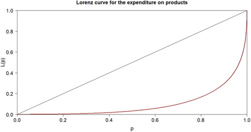
Given the characteristics of the hypothesis we want to prove, some information about the expenditure on each of the 7,572 different products is also provided. Figure 1 shows a histogram for the total expenditure over these 50 months on every product of this company. Figure 2 shows the Lorenz Curve as a measure of inequality on the expenditure of these products.

Figure 1. Bar plot of the absolute frequency of the total amount of expenditure per product.

Source: Authors.

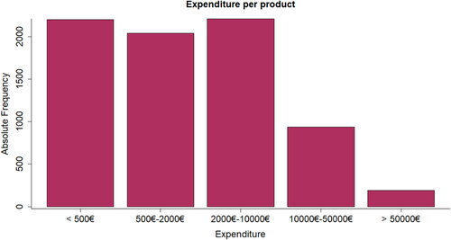
Figure 2. Lorenz curve for the distribution of the expenditure on the different products.

Source: Authors.

These two figures reveal that there is a great deal of inequality on the income that every product brings to the company. In Figure 1, we can observe that most of the products (almost 90%) generated less than €10,000 of sales during the period. Then, around 900 other products generated quite a larger amount (between €10,000 and €50,000 each) while almost 200 products brought more than €50,000 each.

These numbers lead to the inequality distribution shown in Figure 2 where it can be observed that the Pareto principle almost holds: 20% of the products are responsible of 80% of total income. The Gini index for the expenditure on every product is 0.804 which means quite a great deal of inequality regarding the income brought by each SKU. Although measuring inequality among the expenditure within the different products of the catalogue is not an objective of this paper, we found it useful for the reader in order to obtain a quick idea of how the company generates its revenues.

3. Key concepts and literature review

3.1. Heterogeneity measurements

Shopping basket heterogeneity is not a variable that can be quantified in a trivial way so there is a need for some discussion about what this concept means and how it can be measured. As defined by Boztuğ and Reutterer (2008), we understand a shopping basket as the set of items (or product categories) included in a retail assortment that a consumer purchases during one and the same shopping trip. Nevertheless, although we agree with the convenience of the definition, we will consider the items bought during a certain period instead of the items bought within the same shopping trip. We proceed this way because our interest is to check the variety of products the clients are purchasing over time and not to analyse the shopping basket of one specific purchase.

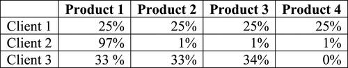
First, we provide a practical example of how we understand heterogeneity within a client’s shopping basket. To make it simpler, let’s consider a business offering four different products and let’s consider the historical shopping basket (in terms of the percentage of items of each product bought during the period over the total amount of products) of three different clients:

In this situation, we understand that Client 1 is the most heterogeneous since he or she buys all the products and he or she does so in the most heterogeneous way possible. Client 2 also bought all the products available, but his or her level of diversity is very low provided that the great majority of purchases come from the same product. Finally, Client 3 does not buy all the items, but shows a great deal of heterogeneity over those products he or she is buying. From this simple example and forgetting about measurement methods, we would say that Client 1 is the most heterogeneous while Client 2 is the most homogeneous.

The question that arises now is the following: how can we measure this idea? The concept of heterogeneity is particularly relevant in many fields. For instance, it has been commonly used in thermodynamics, ecology, and statistics (among others) where it is called disorder, diversity and information respectively.

To check some examples of how this concept has been applied and measured in the fields we have just mentioned, one can refer to Ozawa et al. (2003) in the context of thermodynamics, Banavar et al. (2010) for an application in ecology and Eliazar and Sokolov (2010) from a statistical perspective.

Nevertheless, what is generally common among all those fields is the regular use of the so-called entropy function to measure them. It is important to highlight that other measures regarding diversity or heterogeneity have been used in many different contexts. For example, one can check Rocchini et al. (2017) for the Rao’s Q Diversity Index or Guiasu (1986) for the weighted entropy among others.

However, as we will properly detail in Section 5, we consider the entropy formula to be the most convenient for our purpose, since it takes into account both the quantity of different items bought during a period and also the proportion that each of these items represent over the total shopping basket. Looking back at Figure 3 and its explanation, one can figure out that this is exactly how we understood heterogeneity: not only a mere count of the number of different items but also their overall weight.

Figure 3. Example of different customer baskets to illustrate the concept of heterogeneity.

Source: Authors.

3.2. Churn prediction

The secondary objective of this article is to prove the significance of a variable that has been constantly missed when building churn models: shopping basket heterogeneity. First, it is important to remark that churn models need to be accommodated to the nature of the company.

Here, we can set an important difference. On the one hand, we have one-service industries (such as telecommunications services, gymnasiums, banks, insurance companies, etc) where it is very common to establish a contractual relationship with the client and, therefore, his or her defection is observable. On the other hand, we have companies offering a wide range of different products to their customers (such as supermarkets, cloth stores, wholesalers selling to retailers, e-commerce sites, etc). In this last setting (non-contractual), the client does not communicate his or her defection and the only evidence to predict this is a suspiciously long hiatus in his or her buying pattern.

On those one-service businesses, testing the accuracy of any churn model over a specific sample is trivial because the response variable (i.e. defection) is completely certain. Hence, the challenge in respect to these models is to choose the correct variables and apply the most accurate method (e.g., logistic regression, neural networks, decision trees, etc.) There is plenty of literature about these kinds of models. For instance, Neslin et al. (2006) talks about the relevance of method selection in terms of predictive accuracy and Verbeke et al. (2011) provides an interesting summary table about the research done on this topic so far.

However, churn models in non-contractual settings are more complicated. To the challenges mentioned before there is also the inconvenience of the lack of awareness on the response variable. The presence of these types of churn models in the literature is not so large compared to the above-mentioned setting.

One of the most revolutionary approaches to targeting this inconvenience is the Pareto-NBD model introduced first by Schmittlein et al. (1987). The usefulness of the model lies in the little data required (frequency, recency and observation period) to estimate the probability of a customer being inactive at a certain time. Many authors have used and tried to improve the Pareto-NBD model afterwards (Reinartz & Kumar, 2000, Hopmann & Thede, 2005 or Abe, 2009 and Mzoughia et al., 2017 using Bayesian approaches).

Another approach with a larger number of explanatory variables that has been developed is the one by Buckinx and Van den Poel (2005). They used up to 61 predictors (related to customer behaviour and demographics) to assess partial defection in the FMCG retail sector.

More examples of models trying to estimate churn in non-contractual settings can be found at Tamaddoni et al. (2010) where they work with a pre-paid mobile telecom company database to predict defection based on customer behaviour (number/type/duration of calls, cost, etc).

Most of the churn measurements in non-contractual settings mentioned above have been tailored specifically for the problem they were trying to approach. However, the advantage of the Pareto-NBD model is its robustness when applying it to any kind of business, since it just considers the time since the last purchase of a customer (recency) considering his usual buying pattern (frequency). More details of how this model predicts churn probability will be specified in Section 4.

3.3. Market basket analysis

Market basket analysis or association rule-mining is a method consisting of discovering customer purchasing patterns by extracting associations or co-occurrences from a store’s transactional databases, Chen et al. (2005). More specifically, it has the objective of identifying products or groups of products, which tend to occur together in buying transactions, Trnka (2010).

According to Kaur and Kang (2016) the main utility of Market Basket Analysis in marketing is to provide the information to the retailer to understand the purchase behaviour of the buyer, which can help this retailer in correct decision making. By knowing which set of items are usually bought together, it becomes easier to approach our customers with more attractive promotions rather than offering them random discounts for random products.

In Karthiyayini and Balasubramanian (2016), some specific situations that use these kinds of algorithms and which will become useful in a business context are mentioned and some of them are listed below:

• Store layout: Put products that co-occur together to improve the customer shopping experience.

• Marketing: Target customers who can potentially be interested in a product. Then, attract these targeted customers with promotions to encourage them to spend more on their shopping basket.

• Online retailers: Drive recommendation engines like Amazon or many other online stores.

There are several algorithms to perform Market Basket Analysis. Probably, the most popular is the Apriori algorithm developed by Agrawal and Srikant (1994) which has been implement in the statistical software R. The implementation allows even non expert users to obtain interpretable results since the required information (and its format) is easy to obtain and the code is intuitive enough. More details about the algorithm and specially about some important concepts regarding Market Basket Analysis will be given in Section 6.3 together with the summary of the results of the algorithm.

4. Measuring churn in non-contractual settings: the pareto-NBD model

Defection of a client is a variable that is not always observable. Particularly, in those businesses where no contract is set between the supplier and the buyer, a company has no tool to determine if a customer has finished its relationship with them. In fact, the only evidence that may prove this defection is a buying hiatus longer than expected considering its traditional transaction pattern.

Knowing the nature of the business where the company operates, one can aim to design a tailored model to detect churn in these circumstances. However, the Pareto-NBD model introduced by Schmittlein et. al. (1987) uses an approach that makes sense for any kind of business.

The only information this model needs to compute the probability that a client is still active is the number of purchases (x), the moment when the last purchase occurred (t) and the observation period (T). With just these three variables, we can establish the recency (T-t) and the frequency (T/x) of a particular client.

Those are the five assumptions about the purchase event process and the time the customer stays active (alive) as they were stated first in Schmittlein et al. (1987):

1. Poisson Purchases: While alive, each customer makes purchases according to a Poisson process with rate $\lambda .$

2. Exponential Lifetime: Each customer remains alive for a lifetime which has an exponentially distributed duration with death rate μ.

3. Individuals’ Purchasing Rates Distributed Gamma: The purchasing rate $\lambda$ for the different customers is distributed according to a gamma distribution across the population of customers.

4. Death Rates Distributed Gamma: The customer’s death rates μ are distributed according to a different gamma distribution across customers.

5. Rates $\lambda$ and μ are independent: The purchasing rates $\lambda$ and the death rates μ are distributed independently of each other.

Since careful exploration of this model is not the aim of this article, for the statistical sense and justification of these assumptions, we suggest reviewing the original paper.

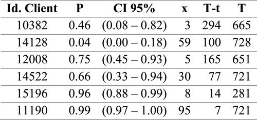
Just as an example of the results of this model concerning the probability that a customer is still active; Figure 4 shows the data and the output of some selected clients in order to illustrate how it works. However, we will make three quick clarifications about the model estimation:

Figure 4. Frequency, recency, observation time, point estimate probability of being alive and its credible interval for some selected clients using the Pareto-NBD model.

Source: Authors.

1. The model was estimated using a Bayesian approach (this is the reason why we can have credible intervals for the probability of being alive in Figure 4).

2. Only the last two years of activity were considered.

3. Because of (2), the number of clients left for analysis decreased to 1,466.

We have deliberately chosen these clients in order to have some with low probabilities of being active, moderate probabilities of being active and high probability of being active respectively for high frequency customers (averaging more than one purchase per month) and low frequency customers (averaging less than one purchase per month). This will help us to understand if the model is bringing sensible estimates for their probability of being active.

First, we analyse the first two customers whose probability estimates of being active are below 50%. The first one has not been active for almost a year (when he or she made three purchases the year before) while the second one was buying, on average, almost once every 10 days and now he or she has been inactive for 100 days. Therefore, in the first case, the wide confidence interval suggests that the model is not sure whether the customer is still alive while the second one has both a point estimate and a credible interval very close to 0, suggesting that the permanent inactivity of the customer is almost granted.

For the third and the fourth client respectively, we can observe point estimates of the probability of being active which are moderately high and wide confidence intervals. The model is quite dubious about the activity of those clients. This seems sensible since the recency of both is higher than their usual average inter-purchase time, but not by a significant amount compared to the two previous cases. Considering that inter-purchase time follows an exponential distribution (because the purchases follow a Poisson process), which is rather skewed to the right, makes sense for the model to hesitate about the activity of these customers.

Finally, the last two clients do not need any detailed comment. Both have bought recently and, therefore, the only evidence the model may have about their inactivity (which is a suspiciously long hiatus) does not exist. Point estimates and credible intervals of both are very close to 1.

The little information required by the model and the simplicity of the assumptions (using 1-parameter distributions such as the Poisson and the Exponential) imply a great deal of simplification on a complex problem such as estimating churn. However, these estimations are sensible and reliable and, although their accuracy might be improved by adding some complexity, it seems clear that the Pareto-NBD model is, at least, useful to order clients in terms of their probability of being active regarding their recency and frequency.

5. Measuring customer basket heterogeneity: Shannon’s entropy

In the introduction, we highlighted two potential obstacles to verify our hypothesis corresponding to the secondary objective, which states that customer basket heterogeneity may have an impact on client defection. In Section 4, we have dealt with one of the obstacles: how to measure the probability of a client being alive (which needs to be understood as the complementary probability of churn) at any moment in time. Now, we need a measurement for that basket heterogeneity both to respond to our primary objective and to overcome the second obstacle.

In Section 3, we have briefly mentioned how other disciplines aside from Marketing measure similar concepts. However, the attempt to measure how diverse a client is when choosing from a wide catalogue has not been specifically addressed yet. At first, our intention was to measure this dispersion just by counting how many different products the customer has bought during a specific period of time. Although this looks reasonable, it might not give the desired results.

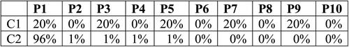
For example, consider these two customers baskets regarding all the 10 products a company offers:

If the method used to measure basket heterogeneity was just to count how many different products the client has purchased, both would score 5. However, we consider this measurement not to be convenient since Client 2 is buying Product 1 almost exclusively (and some other products very occasionally). For example, it could be the case of a client that only regularly buys a single product from us and occasionally (e.g., when the other supplier he or she uses to buy runs out of the other products) some other references from our catalogue.

Contrary to this case is Client 1 who regularly buys five different products from us and can be considered a loyal customer in all these five references. Therefore, it does not make sense to consider a measurement such as just counting the different number of SKUs a client is purchasing. The proportion of each of the references over the whole basket should be also considered.

Following this intuition and reviewing what has been done in other disciplines to measure similar ideas, we found the concept of entropy, firstly introduced by Shannon (1948). Although at the beginning, it was used in Communication Theory, it has been adapted to other fields such as Statistical Thermodynamics or Ecology. Generally, entropy is associated with concepts such as disorder or uncertainty. After Shannon, other different versions of the original entropy formula such as Rényi’s entropy or Hartley’s entropy have been developed.

Nevertheless, the original function serves our purpose of measuring the heterogeneity of a shopping basket in the way we wanted, since it considers not only the number of different references that have been purchased, but also their proportion over the whole basket. The formula, as stated in Shannon (1948), is the following: (1) $$H=\mathrm{}-\mathrm{}\sum _{i=1}^n{p}_i\mathrm{*}{\log }_2{p}_i$$(1) where, adapted to our situation, n would be the total number of different articles purchased by our client and $p_i$ the proportion that represents the article i over the whole basket.

Derived also from Shannon’s manuscript, we can reproduce the most important properties of that formula:

1. $H$ = 0 if and only if all the $p_i$ but one are zero, this one having the value unity.

2. For a given n, $H$ is a maximum and equal to log n when all the $p_i$ are equal (i.e., $\frac{1}{n}$).

The base used for the logarithm is not an important issue since it is just a matter of scale. Our choice for this base is 2, but one can also choose Euler’s number or 10. In fact, we should not forget that we are trying to measure something intangible, therefore, we are much more interested in a measurement that is able to sensibly order and separate our clients in terms of heterogeneity rather than a measurement that brings accuracy, since we have no clue about what accuracy is in this context.

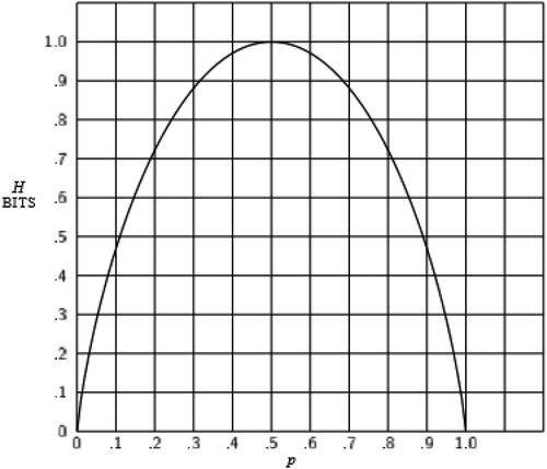
So, just to have an idea of how the formula works we can study its value for the simplest case where a company offers just 2 products. In Figure 5, we reproduce one of the plots of Shannon (1948) to illustrate the relationship between the entropy ($H$) and ${\mathrm{p}}_{\mathrm{i}}.$

Figure 5. Shannon’s entropy in terms of pi when a business offers just two products.

Source: Authors.

We can observe that the entropy reaches its maximum ($H=1)\mathrm{}$ when we reach the highest level of uncertainty ($p_i=0,5$). Moreover, the entropy has two minima ($H=0)\mathrm{}$ which are obviously equivalent ($p_i=0\mathrm{}or\mathrm{}{p}_i=1$).

We can also compute the entropy (1) for the two example customers displayed in Figure 6. $$E_{\mathit{Client}1}=\mathrm{}-5\mathrm{*}(0,2\mathrm{*}{\log }_{2}0,2)=2.32$$ $$E_{\mathit{Client}2}=\mathrm{}-(0,96\mathrm{*}{\log }_{2}0,96)-4\mathrm{*}({0,01\mathrm{*}\log }_2\mathrm{}0,01)=0.32$$

Figure 6. Example of different customer baskets to illustrate the inconveniences of one possible method to measure heterogeneity.

Source: Authors.

This measurement gives a much more realistic idea of how heterogeneous both customers are in terms of their shopping baskets, since it also incorporates the information of the proportion that each item represents over the whole basket.

Although it looks as if we have found a good measure for heterogeneity, there is another difficulty to overcome. How do we calculate these proportions? In terms of the quantity purchased (number of units of the same item) or in terms of the amount of money they represent over the total?

The issue in the sector of wholesalers of beauty products (and in the great majority of businesses) is that their catalogue has some very cheap products that retailers often buy in very large quantities (e.g., hair clips) and some very expensive products that they buy very occasionally (e.g., specialized furniture for hairdressing salons).

Therefore, measuring these proportions $p_i$ with quantities would over-represent those hair clips while assessing it by the amount of money they suppose over the total would over-represent that hairdresser shop furniture. To solve this problem, we have decided to compute the mean between the two types of entropies. So, the final formula used to define the heterogeneity of each client is: (2) $$H^{\mathrm{\text{'}}}=0,5\mathrm{*}\left(\mathrm{}-\mathrm{}\sum _{i=1}^n{q}_i\mathrm{*}{\log }_2{q}_i\right)+0,5\mathrm{*}\left(\mathrm{}-\mathrm{}\sum _{i=1}^n{m}_i\mathrm{*}{\log }_2{m}_i\right)$$(2) where:

$q_i$ is the number of units bought from an item over the total quantity of units bought and $m_i$ is the amount of money spent on an item over the total amount of money spent on all items.

6. Results

In this section, we are going to show the main results derived from the 3 different objectives we established at the beginning of the paper: building a measurement for shopping basket heterogeneity, checking its possible relationship with churn and using Market Basket Analysis to improve the profitability of those low-heterogeneity customers.

6.1. Overview of the results for the H’ measurement

To calculate this heterogeneity defined in (2), all the items bought during the period mentioned in Section 2 (from January 2014 to March 2018) have been considered to define every customer shopping basket.

To provide a summary of the results obtained at a customer-level, we show, in Figures 7 and 8 respectively, how the distribution of heterogeneity falls over our sample of 1,466 customers that have made at least a couple of purchases over the last two years (Section 4).

Figure 7. Histogram of H’ over the 1.466 customers of the company who purchased at least twice during the last two years.

Source: Authors.

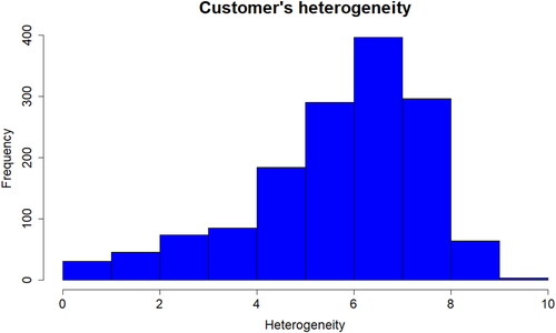
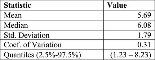
Figure 8. Some descriptive statistics of the distribution of H’.

Source: Authors.

As we have already mentioned in this section, it is not possible to state whether the results are accurate or not. What we want to measure is a concept. Therefore, the objective is that the measurement reasonably orders the customers from the least heterogeneous to the most heterogeneous. Just to quickly check if the measurement provides results which are aligned to the idea of heterogeneity we have previously described, in Figure 9 we have a short summary of the composition of the shopping basket of 3 clients, scoring respectively a low value of H’, a medium value of H’ and a high value of H’.

Figure 9. Client ID, H’ score, number of items bought and what percentage over the total the product with the greatest importance represents (in terms of quantity and expenditure respectively).

Source: Authors.

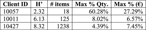
Although, obviously, this is a huge simplification of the results, we found it quite illustrative to show the information displayed in Figure 9. Above, we can clearly differentiate 3 types of clients in terms of heterogeneity. The first one has only purchased 18 different references over the total of 7,572 the company is offering in the catalogue. Furthermore, in terms of quantity, there is a reference which concentrates more than half of the total items bought during the specified period and has a H’ score equal to 2.32. Then, the second one has purchased a considerably higher amount of different references and none of them represents more than 10% of the total, neither in terms of quantity nor in terms of expenditure and scores 6.13 in the H’ measurement. Finally, the last client scores 8.32 in H’ and, as we can see, it as a really heterogeneous client. During the period considered, he has bought more than 1,000 different references and, as we can observe in the last two columns, none of them represents a significantly large amount over the total.

After this short analysis, we are ready to confirm that the measurement we have built is capturing the idea we have previously illustrated a couple of times during the article. Regardless of the scale, which right now does not concern us, the formula we are using guarantees a sensible ordering of the clients in relation to the concept of shopping basket heterogeneity.

6.2. Relationship between churn and shopping basket heterogeneity

The first objective of this article was to provide a way to measure customer shopping basket heterogeneity and has been covered in Section 5. Using the data from Sections 4 and 5 where we computed the probability of being active and the heterogeneity respectively for every customer, we are ready to test if there is a significant relationship between these two variables. The reader should keep in mind that the probability of being active obtained through the Pareto-NBD model is just the complementary of the probability of defection (churn).

As both of our variables are numerical and continuous, we have decided to test its relationship with the Pearson’s correlation test. Therefore, our hypothesis is the following: $$\{\begin{array}{c}{H}_0:\rho =0\\ H_1:\rho \ne 0\end{array}$$ where $\rho$ is the Pearson correlation between these two variables.

In Figure 10, we have the main results for this test:

Figure 10. Point estimate, confidence interval (5% significance) and p-value of the Pearson’s correlation test for the probability of being active and the heterogeneity, respectively.

Source: Authors.

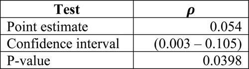
As we can see, our hypothesis has been proved successfully: there are statistical evidences to state that the true correlation (for this particular business) between the probability of a client being active and its heterogeneity is different from 0 (and positive) with a 5% significance.

However, it is also true that the strength of this relationship is quite weak provided that the point estimate as well as the confidence interval is relatively close to 0. Nevertheless, before performing the analysis, we did not expect anything substantially different since we are aware that there is a great number of variables that can explain the defection of a client and the shopping basket heterogeneity is just one of them.

6.3. Market Basket Analysis algorithms

The following step once we have reached the conclusion that heterogeneity may have an impact on churn (as we will discuss in the conclusions, we may need stronger evidence to be sure about this) is to try to increase this heterogeneity for those clients scoring low values. Not only because, if the relationship is true, increasing the heterogeneity of a client would increase the probability that this client remains active, but also because increasing the heterogeneity itself implies increasing the profitability of the customer (the greater the variety of a client’s purchases from the catalogue, the more revenues he or she is bringing to the business).

From now on and to conclude with the results, we will provide a quick and illustrative example of how to use Market Basket Analysis algorithms to try to foster higher profitability from those clients scoring low heterogeneity. To do this, we have used the Arules package in R to use the apriori algorithm. Before proceeding with the results, some key concepts about this type of algorithms are mentioned below (although we suggest reading Agrawal et al. (1993) for more detailed information about association rules techniques as one of the pioneers in this field):

Let X and Y be respectively any set of articles present in our catalogue. Then we can establish the following definitions:

• If we define an association rule such as X ➔ Y, we will call X the left-hand side (LHS) or antecedent and Y the right-hand side (RHS) or consequent. In these conditions, if we consider this as a remarkable association, we will be stating that transactions containing the set of items X tend to also contain the set of items Y but not the other way around.

• Support: The number of times the set of items X and Y appear in a certain transaction divided by the total number of available transactions.

• Confidence: Number of times the set of items X and Y are bought together divided by the support of X. This is the conditional probability of Y given X.

• Lift: This is calculated by dividing the support of X and Y by the product of both supports independently. Values higher than 1 imply a positive correlation between the set of items (and stronger the further we are from 1).

As we said in Section 2, our dataset contains 47,783 transactions that will be taken into consideration to build our association rules. Just to illustrate how we would use the algorithms in order to achieve our objective, we will randomly choose 1 customer scoring low heterogeneity (a value smaller than 2) and we will show which items we should recommend to each customer in order to try to increase his/her shopping basket heterogeneity.

Firstly, the algorithm requires some parameters to define the association rules in terms of support and confidence. We have decided to set a low support (0.005) since the list of transactions (47,783) and references (7,572) available is huge and we have observed it is quite rare to find associations with a higher frequency. Regarding the confidence, our threshold will be 0.2, meaning that we will consider that an association X ➔ Y is interesting if, at least, 20% of the times that the set of items X appear in a transaction also appear the set of items Y. Of course, these two parameters can be tuned depending on the needs of the business.

Hereafter, in Figure 11, we present the association rules obtained for this randomly chosen client which scored a low H’ value.

Figure 11. Association rules for the items bought from a randomly chosen client including: LHS, RHS, support, confidence, lift and count (how many transactions that association includes).

Source: Authors.

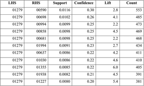
The client we randomly chose had a really low H’ value (1.34) since he only purchased 6 items from the whole catalogue during the observation period (January 2014 until March 2018). Curiously, the apriori algorithm only found LHS associations with 1 of those 6 items he purchased.

So, according to the criteria we have already established, we could somehow encourage this customer to buy some of those 11 items proposed by the algorithm (we previously made sure that none of the items appearing in the RHS were items that have already been bought by the customer). At this point, the marketing actions to convince this customer to purchase the recommended items would need to be designed, but this is not the objective of the current paper.

7. Conclusions, limitations and further research

There are a couple of contributions from this article to the current literature about churn models and consumer behaviour.

First, we have suggested a way of measuring the heterogeneity of the shopping basket of a client. We consider this to be an important magnitude any company should track (obviously, except for those one-service businesses). By knowing how much diversity of our catalogue our customers are purchasing, we have a way to segment our marketing actions towards them.

For instance, a customer with a small degree of heterogeneity might be included in a marketing campaign where he or she is encouraged to purchase other products from the company (e.g., by using Market Basket Analysis algorithms) to increase both his or her loyalty and his or her dependence on our business.

In many cases, a low heterogeneity could mean that our customer is purchasing some items currently being offered by our competition. If we can detect such a situation (our measurement might be a tool for this) and we act accordingly, there is a chance that this customer stops purchasing these products from the competition and starts buying them from us. So, basically, we understand customers with low heterogeneity as those customers that can potentially increase our revenues if they are properly approached. Actually, in our database, the correlation between the heterogeneity and the total expenditure of a customer (over the period stated in Section 2) is significant and its point estimate is 0.18.

Second, we have also proved a significant (although weak) relationship between this shopping diversity and the probability that a customer is still active. As we have mentioned in Sections 1 and 3 churn models that are currently present in the literature do not incorporate heterogeneity as an explanatory variable. Therefore, including this variable constitutes another alternative to improve the accuracy of these models and enrich them.

Talking about the limitations of the research, we should mention the small scope under which this was done. The collection and transformation of data as well as the hypothesis testing has been done only with the information from one company working in a specific sector. Conclusions might be different for other types of businesses and the relationship proved in this article could be either null or stronger for companies working in different scenarios. As stated in the introduction, the main objective was to provide a tool to measure heterogeneity. Nevertheless, if the real interest is to prove this relationship more firmly, data from other companies and sectors must be gathered and tested.

However, it is important to highlight that even if this relationship was weak or even if it is not significant, the Market Basket Analysis makes sense for those clients scoring a low H’ measurement. Precisely, those clients purchasing a lower number of different products are the ones that can potentially increase our revenues by purchasing a larger amount of references.

Besides, there is room to improve research on this same topic. The analysis carried out during the article has been static (i.e., a picture of the situation being taken at a specific moment in time). However, the analysis can be potentially enriched by adding dynamism to the variables. For example, one can compute the heterogeneity every month by taking the information from the last X months to see how this H’ measurement evolves over time and to check whether defection can be partially detected by a gradual decrease on the shopping basket heterogeneity of customers.

Disclosure statement

No potential conflict of interest was reported by the author(s).

References

- Abe, M. (2009). “Counting your customers” one by one: A hierarchical bayes extension to the pareto/NBD model. Marketing Science, 28(3), 541–553. (https://doi.org/https://doi.org/10.1287/mksc.1090.0502
- Agrawal, R., Imielinski, T., & Swami, A. (1993). Mining association rules between sets of items in large databases [Paper presentation]. Proceedings of the 1993 ACM SIGMOD International Conference on Management of Data, 207–216. https://doi.org/https://doi.org/10.1145/170035.170072
- Agrawal, R., & Srikant, R. (1994). Fast algorithms for mining association rules [Paper presentation]. Proceedings 20th International Conference on Very Large Data Bases, VLDB, 487–499.
- Banavar, J. R., Maritan, A., & Volkov, I. (2010). Applications of the principle of maximum entropy: from physics to ecology. Journal of Physics. Condensed Matter: An Institute of Physics Journal, 22(6), 063101. https://doi.org/https://doi.org/10.1088/0953-8984/22/6/063101
- Blattberg, R. C., & Deighton, J. (1996). Manage marketing by the customer equity test. Harvard Business Review, 74(4), 136–144. (
- Boztuğ, Y., & Reutterer, T. (2008). A combined approach for segment-specific market basket analysis. European Journal of Operational Research, 187(1), 294–312. (https://doi.org/https://doi.org/10.1016/j.ejor.2007.03.001
- Buckinx, W., & Van den Poel, D. (2005). Customer base analysis: partial defection of behaviourally loyal clients in a non-contractual FMCG retail setting. European Journal of Operational Research, 164(1), 252–268. (https://doi.org/https://doi.org/10.1016/j.ejor.2003.12.010
- Chen, Y. L., Tang, K., Shen, R. J., & Hu, Y. H. (2005). Market basket analysis in a multiple store environment. Decision Support Systems, 40(2), 339–354. (https://doi.org/https://doi.org/10.1016/j.dss.2004.04.009
- Datta, P., Masand, B., Mani, D., & Li, B. (2000). Automated cellular modelling and prediction on a large scale. Artificial Intelligence Review, 14(6), 485–502. (https://doi.org/https://doi.org/10.1023/A:1006643109702
- Eiben, A., Koudijs, A., & Slisser, F. (1998). Genetic modelling of customer retention. In W. Banzhaf, R. Poli, M. Schoenauer, T. C. Fogarty (Eds.), Genetic Programming. EuroGP 1998. Lecture Notes in Computer Science (Vol. 1391, 178–186). Springer.
- Eliazar, I., & Sokolov, I. (2010). Maximization of statistical heterogeneity: From Shannon’s entropy to Gini’s index. Physica A: Statistical Mechanics and Its Applications, 389(16), 3023–3038. (https://doi.org/https://doi.org/10.1016/j.physa.2010.03.045
- Glady, N.,Baesens, B., &Croux, C. (2009). Modeling churn using customer lifetime value. European Journal of Operational Research, 197(1), 402–411. https://doi.org/https://doi.org/10.1016/j.ejor.2008.06.027
- Guiasu, S. (1986). Grouping data by using the weighted entropy. Journal of Statistical Planning and Inference, 15, 63–69. https://doi.org/https://doi.org/10.1016/0378-3758(86)90085-6
- Hopmann, J., & Thede, A. (2005). Applicability of customer churn forecasts in a non-contractual setting. Innovations in Classification, Data Science and Information, 330–337.
- Karthiyayini, R., & Balasubramanian, R. (2016). Affinity analysis and association rule mining using apriori algorithm in market basket analysis. International Journal of Advanced Research in Computer Science and Software Engineering, 6, 241–246.
- Kaur, M., & Kang, S. (2016). Market basket analysis: Identify the changing trends of market data using association rule mining. Procedia Computer Science, 85, 78–85. https://doi.org/https://doi.org/10.1016/j.procs.2016.05.180
- Mzoughia, M. B., Limam, M., & Borle, S. (2017). A MCMC approach for modeling customer lifetime behavior using the COM-poisson distribution. Applied Stochastic Models in Business and Industry, 34(2), 113–127. https://doi.org/https://doi.org/10.1002/asmb.2276
- Neslin, S. A., Gupta, S., Kamakura, W., Lu, J., & Mason, C. H. (2006). Defection detection: Measuring and understanding the predictive accuracy of customer churn models. Journal of Marketing Research, 43(2), 204–211. (https://doi.org/https://doi.org/10.1509/jmkr.43.2.204
- Ozawa, H., Ohmura, A., Lorenz, R. D., & Pujol, T. (2003). The second law of thermodynamics and the global climate system: A review of the maximum entropy production principle. Reviews of Geophysics, 41(4), 1–24.
- Pfeifer, P. E. (2005). The optimal ratio of acquisition and retention costs. Journal of Targeting, Measurement and Analysis for Marketing, 13(2), 179–188. (https://doi.org/https://doi.org/10.1057/palgrave.jt.5740142
- Reichheld, F. F., & Sasser, E. (1990). Zero Defections: Quality Comes to Services. Harvard Business Review, 68, 105–111.
- Reinartz, W., & Kumar, V. (2000). On the profitability of long-life customers in a noncontractual setting: An empirical investigation and implications for marketing. Journal of Marketing, 64(4), 17–35. (https://doi.org/https://doi.org/10.1509/jmkg.64.4.17.18077
- Reinartz, W., Thomas, J. S., & Kumar, V. (2005). Balancing acquisition and retention resources to maximize customer profitability. Journal of Marketing, 69(1), 63–79. (https://doi.org/https://doi.org/10.1509/jmkg.69.1.63.55511
- Rocchini, D., Marcantonio, M., & Ricotta, C. (2017). Measuring Rao’s Q diversity index from a remote sensing: An open source solution. Ecological Indicators , 72, 234–238. https://doi.org/https://doi.org/10.1016/j.ecolind.2016.07.039
- Schmittlein, D. C., Morrison, D. G., & Colombo, R. (1987). Counting your customers: Who are they and what they will do next? Management Science, 33(1), 1–24. (https://doi.org/https://doi.org/10.1287/mnsc.33.1.1
- Shannon, C. E. (1948). A mathematical theory of communication. Bell System Technical Journal, 27 (4), 623–656. https://doi.org/https://doi.org/10.1002/j.1538-7305.1948.tb00917.x
- Tamaddoni, A., Mehdi, M., Teimourpour, B., & Choobdar, S. (2010). Modeling customer churn in a non-contractual setting: The case of telecommunication service providers. Journal of Strategic Marketing, 18(7), 587–598. (https://doi.org/https://doi.org/10.1080/0965254X.2010.529158
- Trnka, A. (2010). Market basket analysis with data mining methods [Paper presentation]. International Conference on Networking and Information Technology, IEEE, 446–450.
- Verbeke, W., Martens, D., Mues, C., & Baesens, B. (2011). Building comprehensible customer churn prediction models with advanced rule induction techniques. Expert Systems with Applications, 38(3), 2354–2364. (https://doi.org/https://doi.org/10.1016/j.eswa.2010.08.023
- Wei, C., & Chiu, I. (2002). Turning telecommunications call details to churn prediction: A data mining approach. Expert Systems with Applications, 23(2), 103–112. (https://doi.org/https://doi.org/10.1016/S0957-4174(02)00030-1