How much would it cost to eliminate the at-risk-of-poverty rate? Evidence from the European Union

Abstract

The aim of this paper is to assess the cost of eliminating the at-risk-of-poverty rate, based on the Lorenz curve approach (the Gini coefficient, the Kakwani progressivity coefficient). A set of new equations that allow to find a link between cost of closing the relative poverty gap and income inequality is proposed. The main finding is that, after the initial allocation of social benefits, the share of benefits that are still needed to close the relative poverty gap in the pre-government income is a function not only of the at-risk-of-poverty rate, but also of the relative poverty line, the Gini coefficient of income of the poor, and the Kakwani progressivity coefficient of extra benefits. The empirical application of the methodology adopted is illustrated with the use of EU household sample (the data is derived from the EU-Survey on Income and Living Conditions). In line with the suggested decomposition, in the research sample ranking countries according to the at-risk-of-poverty rate does not coincide with the way they are sorted by the share of extra benefits.

Keywords:

• the at-risk-of-poverty rate
• cost of closing the poverty gap
• the Gini coefficient
• the Kakwani progressivity coefficient

JEL CODES:

• C10; D31; D63; E62; H23

1. Introduction

The at-risk-of-poverty rate is the share of the population with disposable income below a predefined poverty line; hence it is a relative poverty measure, contrary to absolute poverty indices. The matter of decreasing or even eliminating relative poverty, along with social exclusion, has been an issue of economic concern for decades in Europe (as well as one of the key targets of social policy).

This paper focuses on the question: how much would it cost to eliminate the at-risk-of-poverty rate? The attempt to find an answer is of fundamental importance for economists. As such, the question has been partially covered in the literature, particularly in reference to income redistribution through social transfers. As a result, we know an equation which enables us to determine the total expenditure that should be incurred in the effort to eliminate relative poverty. However, the spending equation does not provide for inequality in the distribution of household income. This study aims to fill this gap. Especially now it is worth identifying the precise relation between the amount of money required to close the relative poverty gap and the widely used income inequality measures, when increasingly detailed statistics are available on income distribution and redistribution. The findings may be also of high importance while looking deeply into the idea of a guaranteed minimum income, as this concept has been gaining increasing interest.

In this study, to determine the social spending still necessary to overcome the relative poverty gap, the Lorenz curve approach, including income distribution parameters, is used. A set of new equations that allow to find a link between the total cost of closing the relative poverty gap and income inequality is suggested. Unit data are derived from the EU-Survey on Income and Living Conditions 2018 (EU-SILC), which is the largest harmonised database on representative sample of European households (the survey is coordinated by Eurostat). The empirical application of the methodology adopted is illustrated with the example of countries which have low-, middle- and high-ranking position in terms of the relative poverty level (in total, 10 countries are analysed). The at-risk-of-poverty rate that is inspected is defined with regard to households, although the indicator is usually calculated with respect to persons.

It is important to stress that in order to calculate the total cost of closing the relative poverty gap, first, the actual at-risk-of-poverty rate is determined in reference to the national median disposable income after social transfers. Then, all households that are relatively poor are hypothetically granted additional social benefits designed to overcome the problem. Thus, the public funds that are needed to eliminate the relative poverty are calculated under the assumption that an actual allocation of social transfers is a baseline situation, with no reference to the effectiveness of this allocation.

The main finding of this paper is that the share of additional benefits yet to be given in order to close the relative poverty gap in the pre-government income is a function of not only the at-risk-of-poverty rate, but also of the relative poverty line, the Gini coefficient of disposable income of the poor, and the Kakwani progressivity coefficient of extra benefits. Consequently, it does not have to be true that countries with a higher the at-risk-of-poverty rate always need a higher share of extra benefits. This is also why ranking countries according to the at-risk-of-poverty rate does not have to coincide with their classification based on extra social transfers expressed as a percentage of current social spending.

The rest of the paper is laid out as follows. In Section 2, a review of the literature is provided. Section 3 presents the theoretical approach that has been applied. Section 4 describes the empirical sample used. Section 5 reports the empirical research results. Section 6 offers conclusions. In Annex, a list of variables that appear in Section 3 is given.

2. A review of the literature

The literature on redistributive impact of the tax-benefit systems in Europe is substantial. Most of the studies conclude that countries with high original income inequality do not tend to have more redistributive fiscal systems (Causa & Hermansen, 2018; Figari & Verbist, 2013; Paulus et al., 2009; Wagstaff et al., 1999; Zaidi, 2009). Concerning the most recent works on links between the tax-benefit system and the poverty level, Agostini et al. (2016) analysed the impact of tax-benefit policy reforms on income distribution in the EU in 2008–2015. They found that the policy changes were poverty-reducing in total, although variations across the member states were considerable. In 2014–2015, tax and benefit policy changes turned out to be mostly poverty-reducing in Estonia, Belgium, and Finland, whilst they were poverty-increasing in Greece and Latvia (in other countries, the effect was not statistically significant).¹

As regards the subject matter of this paper, it should be pointed out that the problem of the entire sum to be paid to compensate exactly for the poverty gap has already been partially covered in the relevant literature.

Vandenbroucke et al. (2013) calculated the redistributive effort required to guarantee that all EU citizens had income equal to the national poverty threshold. The effort was expressed as a proportion of the non-poor household disposable income that was above the poverty threshold (not all net income of non-poor families). It was assumed that the targeted social transfer from poor families to rich families was costless, in the sense that it did not create any behavioural responses on the part of the groups considered. The redistributive effort varied between the EU countries from 1.1% to 4.6% if the poverty threshold was to be at 60% of the national median disposable income, and it fluctuated in the range 0.2–1.4% if the poverty line was to be at 40% of the national median.

Referring to the working-age population in the EU, Cantillon et al. (2014) showed that current reduction in the at-risk-of-poverty rate due to social transfers was from 3% to 5% in Spain, Greece, Estonia, and Latvia to about 10% in the Czech Republic, Denmark, France, Slovenia, Finland, and Sweden. Regarding only households with members aged 20–59 years, the total cost of increasing all minimum incomes to 60% of the national median disposable income would be 1–2% of household total disposable income (the net income of the total population in question). If the poverty threshold was to be set at 40% of the national median, the financial impact would be in the range 0.07–0.94%.

The above-mentioned studies were improved by Collado et al. (2017), as those authors assessed the cost of closing the poverty gap between the poor and non-poor families, while maintaining average incentives to participate in the labour market. That is to say, this research reflected an awareness that additional social benefits required to compensate exactly for the poverty gap potentially weaken work incentives at the bottom part of income distribution. The results presented referred to Belgium, Denmark, and the United Kingdom (well-developed welfare states with differing welfare regimes), and they indicated that the cost of closing the poverty gap without worsening average participation incentives would be around two times the costs of raising all incomes to 60% of the national median disposable income.

In some other papers, the issue of closing the relative poverty gap experienced by specific social groups such as households with children or the elderly was addressed; see, for example, the work of Atkinson et al. (2002), Levy et al. (2007), and Vandeninden (2012).

Milanovic (2000) used the median-voter hypothesis to describe the relation between income inequality and social spending that induces income redistribution, but the research referred to the inequality of factor income. Alesina and Rodrik (1994), as well as Persson and Tabellini (1991), gave theoretical explanations for the mechanism through which an increase in income discrepancy generates pressure on public authorities to increase pro-poor social expenditure (more generally, the authors described potential links between income inequality and budgetary deficits and, consequently, public debt). Creedy and Moslehi (2011) investigated interactions between income inequality and the composition of public expenditure, showing that income discrepancy affects the degree to which public expenditure is allocated between income-equalising transfer payments and public goods. According to these authors, this result holds in the case of all three decision mechanisms that were considered: majority voting, stochastic voting, and maximising social welfare function.

In his paper, providing distribution-free asymptotic confidence intervals and statistical inference for additive poverty indices, Kakwani (1993) gave a straightforward formula that accounted for the poverty gap: $$\mathit{PGR}=\frac{H(z-\mu )}{z},$$ where $\mathrm{PGR}$ is the poverty gap ratio, $\mathrm{H}$ is the poverty rate, $\mathrm{z}$ denotes the poverty line, and η represents the mean income of the poor. Using this formula, it is possible to derive the total expenditure required to close the poverty gap, and the expenditure is equal to: $$\mathrm{TE}=\mathrm{}{\mathrm{N}}_1\left(\mathrm{z}-\mathrm{\eta }\right)={\mathrm{N}}_1\overline{\mathrm{B}},$$ where ${\mathrm{N}}_1$ is the number of persons below the poverty line and $\overline{\mathrm{B}}$ represents the mean compensation for the relatively poor. As a result, average expenditure in the whole population amounts to $H(z-\mu ),$ that is, it depends on the at-risk-of-poverty rate.

Therefore, relying on the above research, we can determine the total and average expenditure needed to eliminate relative poverty, but these expenditures are based solely on the poverty rate, the poverty line, and the mean income and social transfers. The spending equation does not take into account inequality in the distribution of household incomes, and therefore this paper aims to fill this gap. To achieve this aim, the Lorenz curve approach that provides for disparity in the distribution of household incomes is adopted. It is worth identifying the precise relation between the amount of money required to close the relative poverty gap and the widely used income inequality measures, since increasingly detailed statistics are available on household income distribution and redistribution.² Besides, answering the question of how much it would cost to eliminate the at-risk-of-poverty rate, with special regard to household income discrepancy, may contribute to the discussion on a guaranteed minimum income, as this concept has been gaining increasing interest in recent years.

3. Theoretical approach

Disposable income is defined as: (1) $$Z=X+B-T$$(1) where $X$ is the original income, $B$ denotes social benefits, and $T$ represents income tax: each variable expressed as a mean value. Within the Lorenz curve framework, this relation is related to identity: ${({1+b}_X-t_X)L}_Z\equiv L_X+b_X{L}_B-t_X{L}_T,$ where $b_X$ is average benefit rate, $t_X$ is average tax rate, $L_Z$ is concentration curve of disposable income, $L_X$ is Lorenz curve of original income, and $L_B\mathrm{}$ and $L_T$ are concentration curves of social benefits and income tax, respectively. The average benefit rate is the ratio of benefits to original income, while the average tax rate is the share of tax in original income, that is $b_X=\frac{B}{X}$ and $t_X=\frac{T}{X}.$ The identity is described by Lambert (2001), Lambert and Pfähler (1988), and partially by Kakwani (1977).

To track the link between the total cost of closing the relative poverty gap and income inequality, this paper proposes a set of new equations that are based on observation that the full sample can be divided into two clear-cut groups. The first group of households consists of the units which have disposable income that is lower than a given poverty threshold, whereas the second group is made up of the units that have disposable income that is equal or higher than this boundary line. In other words, the first subsample embodies the units which are at risk of poverty.

So, disposable income in the total sample is: (2) $${Z=Z}_1+\mathrm{}{Z}_2$$(2) where $Z_1$ is the disposable income in the first group of households and $Z_2$ is the disposable income in the second group of households.

Let’s assume that the first group of households is hypothetically granted extra social benefits, and that this is done in such a way that each household is given the exact amount of benefits needed to meet the prespecified poverty threshold. The model posits that additional social benefits are totally tax-free, which yields: (3) $$\overline{Z}=Z_1+B^{\mathrm{*}}$$(3) where $\overline{Z}$ is a hypothetical disposable income that is exactly the same as the poverty threshold and $B^{\mathrm{*}}$ stands for the extra social benefits. As a rule, extra social benefits are granted only to the first subsample of households.

Reverting to the full household sample – that is, both poor and non-poor units – after granting extra benefits, the level of disposable income would be the sum of the following components: (4) $$Z^{\mathrm{*}}=\overline{Z}+Z_2=X+B+B^{\mathrm{*}}-T.$$(4)

The average extra benefit rate in the whole sample would be given by: (5) $$b_X^{\mathrm{*}}=\frac{N_1}{N}\frac{B^{\mathrm{*}}}{X}.$$(5)

Now let’s focus again on the first group of households and notice that the equation (3)(3) $$\overline{Z}=Z_1+B^{\mathrm{*}}$$(3) can be rewritten as: (6) $$Z_1=\overline{Z}-B^{\mathrm{*}}$$(6) and, according to Kakwani (1980), the Gini coefficient of income can be expressed as the weighted average of the concentration coefficient of each factor income component, the weights being proportional to the mean of each factor income: (7) $$G_{Z_1}=\frac{\overline{Z}}{Z_1}{C}_{\overline{Z}}-\frac{B^{\mathrm{*}}}{Z_1}{C}_{B^{\mathrm{*}}}$$(7) where $G_{z_1}$ is the Gini coefficient of disposable income, $C_{\overline{Z}}$ is the concentration coefficient of poverty threshold, and $C_{B^{\mathrm{*}}}$ is the concentration coefficient of extra benefits. As such, the extra benefit concentration coefficient unveils the extent to which the benefit allocation differs from the distribution of disposable income. If allocation of the transfers is unequal over the distribution of the disposable income, in favour of the poorest (richest) households, the benefit concentration coefficient is negative (positive).

The key to current analysis is to notice that, if extra benefits lead to a situation that all households in the first group would have the same disposable income, then the concentration of this income would be equal to zero. Thus, if $C_{\overline{Z}}$ = 0, then the following relationship would hold: (8) $$G_{Z_1}=-\frac{B^{\mathrm{*}}}{Z_1}{C}_{B^{\mathrm{*}}}.$$(8)

Entering Equation (6)(6) $$Z_1=\overline{Z}-B^{\mathrm{*}}$$(6) into Equation (8) and rearranging with respect to $B^{\mathrm{*}}$ yields: (9) $$B^{\mathrm{*}}=\frac{\overline{Z}{G}_{Z_1}}{(G_{Z_1}-{\mathrm{}C}_{B^{\mathrm{*}}})}.$$(9)

Modelling the Kakwani progressivity coefficient of income tax, the progressivity coefficient of extra benefits can be connoted: it is the difference between the Gini coefficient of disposable income and the concentration coefficient of extra benefits: $K_{B^{\mathrm{*}}}$ = $G_{Z_1}-C_{B^{\mathrm{*}}}.$ If the extra benefit concentration coefficient is negative (positive), the extra benefit progressivity coefficient is positive (negative), and positive (negative) extra benefit progressivity coefficient is the factor that contributes to the income inequality reduction (increase). The other factors that determine the income inequality change are average benefit rate and re-ranking (Aronson et al., 1994).

Applying the definition of the progressivity coefficient of extra benefits to the Equation (9), we have: (10) $$B^{\mathrm{*}}=\frac{\overline{Z}{G}_{Z_1}}{(G_{Z_1}-C_{B^{\mathrm{*}}})}=\frac{\overline{Z}{G}_{Z_1}}{K_{B^{\mathrm{*}}}}.$$(10)

Combining formulas (5) and (10), we obtain: (11) $$b_X^{\mathrm{*}}=\frac{N_1}{N}\frac{B^{\mathrm{*}}}{X}=\frac{N_1}{N}\frac{\overline{Z}}{X}\frac{G_{Z_1}}{K_{B^{\mathrm{*}}}}.$$(11)

In summary, the average extra benefit rate – that is, the share of additional benefits required to overcome the problem of relative poverty – is increasing function of the following three variables. First, the at-risk-of-poverty rate itself. Second, the excess of poverty threshold above the original income level. Third, the inequality of disposable income of the poor adjusted for the progressivity of extra benefits.

It is also possible to decompose the Gini coefficient of hypothetical disposable income into the between-groups inequality and the within-group inequality: (12) $$G_{Z^{\mathrm{*}}}=G_{\mathit{between}}+{\partial }_1{G}_{\overline{Z}}+{\partial }_2{G}_{Z_2}.$$(12) where $G_{\mathit{between}}$ is the between-groups disproportionality, ${\partial }_i$ is the product of population share and income share attributed to each subgroup ($i=1,2$), $G_{\overline{Z}}$ is the within group disproportionality in the first group, and $G_{Z_2}$ is the within group disproportionality in the secondgroup. Inter-group inequality is computed by substituting every income in each subgroup with the subgroup mean. This formula is based on the Gini coefficient decomposition: $G=G_{\mathit{between}}+\sum a_K{G}_K+R,$ as it was introduced by Lambert and Aronson (1993). $R$ is a residual that assumes positives values if subgroup income ranges overlap (re-ranking). In our case there is no inequality in the distribution of hypothetical disposable income in the first group of households ($G_{\overline{Z}}=0$) and the subsample income ranges do not overlap ($R=0$), which means that: (13) $$G_{Z^{\mathrm{*}}}=G_{\mathit{between}}+{\partial }_2{G}_{Z_2}=G_{\mathit{between}}+\frac{N_2}{N}\frac{Z_2}{Z^{\mathrm{*}}}{G}_{Z_2}$$(13)

Thus, the hypothetical disposable income Gini coefficient depends only on the between-groups inequality and the inequality within the second group of households.

4. Empirical sample

The sample that is used in this study is taken from household data file in EU-SILC 2018 (the latest data available; the November 2019 release). EU-SILC collects micro data on the income, poverty, social exclusion, and living conditions of Europeans; it is coordinated by Eurostat. The unit data across European countries are harmonised, allowing international comparison of income distribution, as well as income redistribution through social benefits and income taxation. To be precise, the sample that is dealt with in this research refers to 28 European countries, covering 221 549 households in total, but due to data unavailability, information on households in Ireland, the Slovak Republic, and the United Kingdom is for 2017.

For each household in the data set the following three categories of current income were identified: pre-government income (original income or pre-fiscal income), social benefits, and disposable income (final income) (European Commission. Eurostat, 2019).

Pre-government income consists of the following components: gross employee cash or near cash income, gross cash benefits from self-employment, retirement pensions, regular inter-household cash transfers, and income received by people aged under 16 (as defined by Eurostat). Thus, this is income received by all household members with the exclusion of social transfers other than old-age pensions (pensions are counted as original income, since they are understood as deferred income from work).

Except for old-age pensions, social benefits cover all registered benefits: sickness benefits, disability benefits, family-related allowances, housing allowances, education allowances, unemployment benefits and social exclusion not covered elsewhere (only cash social benefits are considered). Obviously, those benefits may directly redistribute income at the household level.

Disposable income equals original income plus social benefits minus tax on income and social insurance contributions. Tax on income includes taxes on individual, household or tax-unit income, as it is registered by Eurostat (it also includes tax reimbursement). For the sake of brevity, tax on income and social insurance contributions hereinafter will be referred to as ‘income tax’.

To consider differences in household size and demographic structure, the modified OECD equivalent scale is used (the scale assigns a value of 1 to the first household member, of 0.5 to each additional adult, and of 0.3 to each child). Consequently, the numerical results presented in this study refer to the distribution of households with respect to income per equivalent unit, contrary to administrative data that usually refer to beneficiaries and taxpayers as being natural persons.

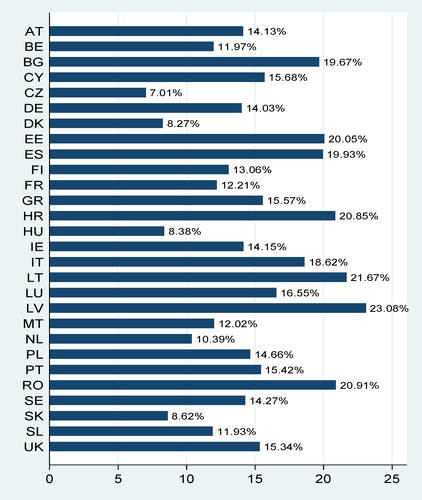
For each country in the research sample, the share of households that have disposable income lower than 60% of the national median equivalised disposable income was determined (the applied poverty line is the one that is most commonly used, but the poverty threshold sometimes is set at 40% or 50% of the national median or mean disposable income). As pointed out in Table 1, the average share of households at risk of poverty was 14.94%. But there was a high degree of heterogeneity among the EU member states, as the lowest level of the variable was 7.01%, and the highest level was 23.08%. The median value was 14.47%. At this point it should be emphasised once again that this indicator is the relative poverty measure that compares the material situation of families within a specific country, but not across the countries (countries with similar share of households at risk of poverty may differ significantly in terms of absolute income of the poor).³

Table 1. The percentage of households at risk of poverty: cross-country summary statistics.

	Obs	Mean	Std. dev.	Min	Max	Median
the at-risk-of-poverty rate	28	14.9449	4.4051	7.0144	23.0801	14.4683

Note: Own calculations based on EU-SILC 2018 data (due to data unavailability, the indicators for Ireland, the Slovak Republic, and the United Kingdom are for 2017). The poverty threshold is set at 60% of the national median equivalised disposable income.

The indicator determined in this research differs from the most common relative poverty measure – namely, the at-risk-of-poverty rate reported by Eurostat. The reason is that the former tells about the percentage of households that are relatively poor, while the latter informs about the share of persons that live in relatively poor households (and that is why the latter is disclosed by Eurostat by age and sex). As long as there is information about the number of family members, it is possible to derive the latter from the former (in fact, both measures take into account the poverty threshold expressed in terms of equivalised disposable income). It would be interesting to discuss the extent to which applying different equivalence scales in this study may change the percentage of households that are relative poor, as parallel analysis has been already conducted (see Bishop et al., 2014).

Of course, European countries vary with respect to relative poverty, as a consequence of variations in inequality in disposable income distribution. The final income inequality in turn is determined by both the inequality in pre-fiscal income distribution and the intensity of income redistribution through social benefits and income tax. However, those complex problems are beyond the scope of this study. To discuss factors contributing to income inequality in Europe, see, among others, A Fiscal Approach for Inclusive Growth in G7 Countries (2017), Atkinson (2013), Borsi and Metin (2013), and Global Wage Report (2018).

The share of population living below the relative poverty line may change within a relatively short time in a specific country, as a result of fluctuations in the poverty threshold defined as the given percentage of the national median or mean disposable income. For example, this happened in some European countries in 2014--2016 when median disposable income went up, mainly due to wage growth (Gasior & Rastrigina, 2017).

Figure 1 allows to see the at-risk-of-poverty rate by country.

Figure 1. The percentage of households at risk of poverty in the EU countries.

Note: Own calculations based on EU-SILC 2018 data (due to data unavailability, the indicators for Ireland, the Slovak Republic, and the United Kingdom are for 2017). The poverty threshold is set at 60% of the national median equivalised disposable income.

5. Empirical research results

Taking into account the total number of countries in the full sample, below are only presented research results for the three countries that have the lowest share of relatively poor households, the three of them that have the highest ratio of such households, and the four of them that have the middle position in the ranking. Countries are chosen in this way for ease of illustrating the empirical application of the methodology presented in Section 3.

Table 2 presents both the number of households in the data set that was used and the percentage of households at risk of poverty. The lowest level of the at-risk-of-poverty rate was found in the Czech Republic (7.01%), Denmark (8.27%), and Hungary (8.38%), whereas the highest was recorded in Latvia (23.08%), Lithuania (21.67%), and Romania (20.91%). Ireland (14.15%), Sweden (14.27%), Poland (14.66%), and the United Kingdom (15.34%) were the middle-ranking countries.

Table 2. Number of households in data set and the share of households at risk of poverty in countries which have low-, middle- and high-ranking position in terms of relative poverty.

	Countries with the lowest share of households at risk of poverty			Countries with the middle share of households at risk of poverty				Countries with the highest share of households at risk of poverty
	CZ	DK	HU	IE	SE	PL	UK	RO	LT	LV
number of households	8454	5390	6263	4536	5640	14853	11702	7088	4687	5702
the share of households at risk of poverty	0.0701	0.0827	0.0838	0.1415	0.1427	0.1466	0.1534	0.2091	0.2167	0.2308

Note: Own calculations based on EU-SILC 2018 data (due to data unavailability, the results for Ireland and the United Kingdom are for 2017).

Table 3 column (1), indicates the ratio of actual social benefits to original income, revealing that it is not necessary for the country to have a high share of benefits to register a low share of households at risk of poverty. For example, the Czech Republic and Hungary (that is, the two countries with a low-ranking position in terms of relative poverty) had a low share of benefits. Ireland, a country with a middle-ranking position, was characterised by the highest average benefit rate, and almost the same conclusion applied to Sweden. The reason is that the actual proportion of families living on an income lower than the pre-specified poverty line is the outcome not only of social transfers that have already been allocated, but also the primary income earned by the household members, as well as the income tax paid by them. Thus, Romania yielded both the third highest relative poverty indicator and an extremely low average benefit rate. Broadly speaking, setting the position of a given country in terms of the at-risk-of-poverty rate against its average benefit rate may help to judge the effectiveness of actual social transfers in reducing relative poverty, but this problem is not covered by this study.

Table 3. The average benefit rate, the average extra benefit rate, and the ratio of poverty threshold to original income.

	(1)	(2)	(3)
	$b_X$	$b_X^{*}$	$\overline{Z}$/X
CZ	0.0410	0.0049	0.4559
DK	0.0553	0.0052	0.3722
HU	0.0495	0.0105	0.4489
IE	0.0832	0.0125	0.4414
SE	0.0760	0.0132	0.4322
PL	0.0516	0.0156	0.4359
UK	0.0521	0.0153	0.4331
RO	0.0197	0.0297	0.4327
LT	0.0622	0.0254	0.4442
LV	0.0577	0.0249	0.4091

Note: Own calculations based on EU-SILC 2018 data (due to data unavailability, the variables for Ireland and the United Kingdom are for 2017).

Assuming a bottom-up equalisation of disposable income of the poor as described in section 3, the average extra benefit rate, i.e. the share of additional benefits required to overcome the relative poverty problem, is reported in column (2) in Table 3. It is easy to see that an increase in the at-risk-of-poverty rate does not have to induce a proportional increase in the average extra benefit rate; for example, Hungary had almost the same the at-risk-of-poverty rate as Denmark, but the average extra benefit rate that was calculated for this country was two times higher. What is more, countries with a lower percentage of relatively poor households may be marked with a higher average extra benefit rate, and this could be seen in the case of Poland versus the United Kingdom, as well as in the case of Lithuania as compared to Latvia. In the research sample, Romania served as an example of a country with high, but not the highest, relative poverty – and which needed the highest share of extra benefits. To understand why ranking countries based on the scope of relative poverty may be different that their classification according to the average extra benefit rate, the formula (11) should be recalled: the rate is determined not only by the share of population living below the poverty line, but also the excess of poverty threshold over pre-government income, and the inequality of disposable income of the poor adjusted for the progressivity of extra benefits. The last two factors will be discussed below.

The ratio of poverty threshold to original income is specified in Table 3, column (3); its lowest level was registered in Denmark and its highest level was found in the Czech Republic. Since the poverty line was set at 60% of the national median equivalised disposable income, and for each country the ratio was less than 0.6, the national median disposable income was lower than the mean pre-fiscal income. This partially bespeaks the degree to which pre-fiscal income was redistributed with the use of the tax-benefit system. Generally, the difference between income tax and social benefits ($T-B)$ is called the net tax, and the following trade-off occurs: the less redistributive net tax is (in favour of underprivileged families), the higher and the more selective extra benefits must be. This should be kept in mind while reforming existing tax-benefit regimes.⁴

The first information in Table 4, namely the disposable income Gini coefficient for households that are below the poverty line, admits that there were substantial variations among the EU member states in the level of this variable (the same as in the case of the share of households at risk of poverty). It is possible for a country to have both a low-poverty rate and a high-final income inequality in the lower tail of income distribution or vice versa. In the research sample, this was the case of Hungary or, on the other spectrum, to some extent, Lithuania and Latvia. Romania was distinguished by both high-relative poverty and high disposable income inequality among the relatively poor families. It would be interesting to extend this study to capture the link between the disposable income Gini coefficient for the poor and for the whole population, as this kind of analysis has already begun. For instance, Leigh (2007) found a strong relationship between top income shares and broader inequality measures, including the Gini coefficient (this suggests that panel data on top income shares may be a useful substitute for other measures of income inequality if other income distribution measures are of low quality or unavailable).

Table 4. The disposable income Gini coefficient, the extra benefit concentration coefficient, the extra benefit progressivity coefficient, the ratio of the Gini coefficient to the extra benefit progressivity coefficient in the first group of households, and additional benefits as a proportion of benefits that have already been allocated.

	(1)	(2)	(3)	(4)	(5)
	$G_{Z_1}$	$C_{B^{*}}$	$K_{B^{*}}$	$G_{Z_1}/K_{B^{*}}$	$\sigma$
CZ	0.0887	−0.4836	0.5723	0.1549	0.1195
DK	0.1033	−0.5039	0.6072	0.1701	0.0940
HU	0.1959	−0.5042	0.7000	0.2798	0.2121
IE	0.1360	−0.5420	0.6780	0.2005	0.1502
SE	0.1307	−0.4775	0.6082	0.2148	0.1737
PL	0.1474	−0.4555	0.6029	0.2444	0.3023
UK	0.1347	−0.4467	0.5814	0.2316	0.2937
RO	0.1993	−0.4066	0.6059	0.3289	1.5076
LT	0.1510	−0.4201	0.5711	0.2644	0.4084
LV	0.1590	−0.4426	0.6016	0.2642	0.4315

Note: Own calculations based on EU-SILC 2018 data (due to data unavailability, the variables for Ireland and the United Kingdom are for 2017).

Column 2 in Table 4 provides concentration coefficient of extra benefits – that is, the transfers that should be directed to relatively poor families to assure they achieve 60% of the national median equivalised disposable income. The coefficient was negative, which confirms that this hypothetical additional support must be given to units with the lowest income. On the other hand, the extra benefit progressivity coefficient, visible in column 3, was higher than zero. As it was calculated as the difference between the disposable income Gini coefficient and the extra benefit concentration coefficient, its positive value indicates that this additional help would force income inequality reduction. The values of coefficients presented in columns 2 and 3 are precisely the ones that guarantee that all households would be given accurate additional benefits so as to have the minimum postulated disposable income.

The ratio of the disposable income Gini coefficient for the poor to the extra benefit progressivity coefficient, that is shown in column 4, was the highest in Romania and Hungary, whereas it was the lowest in the Czech Republic and Denmark.

The above results are more comprehensible if average extra benefit in the whole sample is compared to average benefit in the whole sample, which is equivalent to the ratio of the average extra benefit rate to the average benefit rate ($\sigma =\frac{N_1}{N}\frac{B^{\mathrm{*}}}{B}=\frac{b_X^{\mathrm{*}}}{b_X}$), and this information is given in Table 4, column (5). Strictly speaking, this indicator expresses social benefits yet to be distributed to eliminate the relative poverty as a proportion of social expenditure that actually were incurred. Public funds that were still demanded were equivalent to only 11.95% of the current social spending in the Czech Republic and 9.40% of the current social spending in Denmark. Referring to countries which had a middle-ranking position in terms of relative poverty, that is Sweden and Poland, the index was 17.37% and 30.23%, respectively. As regards Lithuania and Latvia, it was 40.84% and 43.15%, respectively. The worst position in terms of additional expenditure to be incurred as compared to benefits already given referred to Romania, as it was as much as 150.76%.

Table 5 shows the decomposition of the hypothetical disposable income Gini coefficient for the whole sample. Ranking countries according to the share of relatively poor households was inverse to the way they were sorted by the product of population share and the hypothetical disposable income share of the second group of households (column 2). This confirms that, even after giving supplementary benefits to the relatively poor families, the income share assigned to the relatively rich families would doubtless have remained higher (population share was held constant). Just as in formula (13), inequality in distribution of hypothetical disposable income for all units would have resulted only from the between-groups inequality and the inequality within the second group (as there would be no inequality within the first group).⁵

Table 5. The between-groups Gini coefficient of hypothetical disposable income, the product of population share and hypothetical income share of the second group of households, the Gini coefficient of disposable income in the second group of households, the Gini coefficient of hypothetical disposable income, the Gini coefficient of disposable income, and the redistributive effect of extra benefits.

	(1)	(2)	(3)	(4)	(5)	(6)
	$G_{\mathit{between}}$	${(N}_2/N$)/($Z_2$/$Z^{*}$)	$G_{Z_2}$	$G_{Z^{*}}$	$G_Z$	${RE}_{B^{*}}$
CZ	0.0336	0.8959	0.2274	0.2373	0.2442	−0.0283
DK	0.0390	0.8771	0.2269	0.2380	0.2470	−0.0364
HU	0.0391	0.8752	0.2205	0.2321	0.2472	−0.0611
IE	0.0715	0.7983	0.2751	0.2912	0.3086	−0.0564
SE	0.0649	0.7899	0.2052	0.2271	0.2467	−0.0794
PL	0.0708	0.7887	0.2415	0.2613	0.2836	−0.0786
UK	0.0773	0.7822	0.2713	0.2895	0.3112	−0.0697
RO	0.1034	0.7074	0.2478	0.2787	0.3203	−0.1299
LT	0.1152	0.7036	0.3055	0.3302	0.3634	−0.0914
LV	0.1248	0.6876	0.3069	0.3359	0.3706	−0.0936

Note: Own calculations based on EU-SILC 2018 data (due to data unavailability, the results for Ireland and the United Kingdom are for 2017).

Concerning Table 4 once again, namely the verdict that extra social benefits would force income inequality decrease, it is in fact quite easy to calculate potential redistributive effect of those benefits. It is enough to assume that the effect is understood as the relative difference between post-extra benefit and pre-extra benefit income inequality (${RE}_{B^{\mathrm{*}}}=\frac{G_{Z^{\mathrm{*}}}-G_Z}{G_Z}$). The Gini coefficient of hypothetical disposable income and the Gini coefficient of disposable income in the whole household sample are presented in Table 5, columns 4 and 5, respectively. Column 6 gives the hypothetical redistributive effect of extra benefits: the higher the income equalising effect in absolute value, the stronger the income inequality reduction (as those benefits would lead to lower income disproportionality). In absolute terms, the variable ranged from 2.83% in the Czech Republic to 12.99% in Romania.⁶

While interpreting the above results, it should be remembered that hypothetical social benefits were assumed to be totally tax-free. This was a considerable simplification, but it was imposed in order to guarantee the clarity of the current analysis. Across the EU countries, different kinds of benefits are in fact subject to different taxation rules, depending on the particular PIT system. From this point of view, the theoretical approach used in this research may be developed in the future to allow for different taxation schemes of extra social benefits.

The above results show the total cost of eliminating the relative poverty gap, with special reference to income distribution parameters, but they do not take into account relevant behavioural effects. Closing the relative poverty gap through means-tested social transfers may weaken labour force participation, but the existing evidence is rather mixed (Gassmann & Trindade, 2019). On the other hand, such transfers can provide income security, support investments in health, education, culture, etc. To strengthen labour supply incentives, conditional cash transfers may be introduced, such as in work-benefits (in-work payments involving an hours threshold), as has recently been done in several OECD countries.

6. Conclusions

In this paper, the methodology has been introduced for calculating how much it would cost to eliminate the at-risk-of-poverty rate taking into account inequality in the distribution of household income. The approach used allows us to understand that the share of social benefits that are still needed to overcome the relative poverty problem is a function not only of the ratio of households at risk of poverty, but also of the poverty threshold surplus over the original income, and the disposable income inequality of the poor adjusted for extra benefit progressivity (derived from the extra benefit concentration). So, it does not have to be true that countries with a higher the at-risk-of-poverty rate always need a higher share of extra benefits. That is also why ranking countries according to the at-risk-of-poverty rate does not have to match their position based on social transfers yet to be financed expressed as a percentage of their current social spending.

The findings from this paper may add important aspects to the discussion about the basic income system at the national levels, as the results can be helpful in judging the effectiveness of this system in alleviating relative poverty (they can also serve as guidance for designing the adequate minimum wage scheme).

Annex: List of variables that appear in Section 3.

$Z$ - disposable income

$X$ - original income

$B$ - social benefits

$T$ - income tax

$b_X$ - average benefit rate

$t_X$ - average tax rate

$L_Z$ - concentration curve of disposable income

$L_X$ - the Lorenz curve of original income

$L_B$ - concentration curve of social benefits

$L_T$ - concentration curve of income tax

$Z_1$ - disposable income in the first group of households

$Z_2$ - disposable income in the second group of households

$\overline{Z}$ - hypothetical disposable income in the first group of households (the poverty threshold)

$B^{\mathrm{*}}$ - extra social benefits in the first group of households

$Z^{\mathrm{*}}$ - hypothetical disposable income

$b_X^{\mathrm{*}}$ - average extra benefit rate

$N_1$ - number of households in the first group of households

$N$ - total number of households

$G_{z_1}$ - the Gini coefficient of disposable income in the first group of households

$C_{\overline{Z}}$ - concentration coefficient of hypothetical disposable income in the first group of households

$C_{B^{\mathrm{*}}}$ - concentration coefficient of extra benefits in the first group of households

$K_{B^{\mathrm{*}}}$ - progressivity coefficient of extra benefits in the first group of households

$G_{Z^{\mathrm{*}}}$ - the Gini coefficient of hypothetical disposable income

$G_{\mathit{between}}$ - the between-groups Gini coefficient of hypothetical disposable income

${\partial }_i$ - product of population share and income share attributed to the i-th group of households

$G_{\overline{Z}}$ - the Gini coefficient of hypothetical disposable income in the first group of households

$G_{Z_2}$ - the Gini coefficient of disposable income in the second group of households

$N_2$ - number of households in the second group

$\overline{Z_2}$ - mean disposable income in the second group of households

$\overline{Z^{\mathrm{*}}}$ - mean hypothetical disposable income

Disclosure statement

No potential conflict of interest was reported by the author.

Additional information

Funding

This work was supported by the National Science Centre in Poland under Grant ‘Income Redistribution and Public Debt (Statistically Econometric Approach)’ (No. 2013/11/B/HS4/01078).

Notes

1 While comparing the tax-benefit system redistributive effect across different studies, one has to be careful if social transfers include public pensions or not, as this particular issue may substantially change the results obtained.

2 The at-risk-of-poverty rate is sensitive to specific changes in income distribution. To assure a close link between this indicator and income inequality measures, and allow for flexibility in setting different poverty thresholds, the income inequality measure that is chosen should take into account the entirety of income distribution (including both the low and high ends of the distribution).

3 It is also possible to calculate the share of households at risk of poverty before social transfers. Comparing the percentage of households at risk of poverty before and after social benefits enables us to reveal the effectiveness of social spending in reducing the number of families that are relatively poor.

4 In each country in the research sample, the average disposable income was less than the average original income, meaning that the income tax was higher than social benefits (however, this data is not presented here). This finding is in line with other studies on the extent of income redistribution through the tax-benefit schemes which also categorised public pensions as a component of primary income (and not a component of social transfers) (Guillaud et al., 2017; Immervoll et al., 2006; Mahler & Jesuit, 2006).

5 Further, following Lambert and Aronson (1993), the hypothetical final income Gini coefficient can be decomposed as $G_{Z^{*}}=\frac{\sum \sum N_1{N}_2\left|\overline{Z}-\overline{Z_2}\right|}{2N^2\overline{Z^{*}}}+\frac{N_2}{N}\frac{Z_2}{Z^{*}}{G}_{Z_2},$ where $\overline{Z_2}$ denotes the mean disposable income in the second group of households and $\overline{Z^{*}}$ is the mean hypothetical disposable income in the whole sample. From this it can be deduced that the lower the difference between hypothetical disposable income in the first group of households (the poverty threshold) and $\overline{Z_2}$ (in absolute terms), the less unequal the income distribution is.

6 Given the definition of the at-risk-of-poverty rate, hypothetical social transfers would increase the poverty line, though to prevent from necessity to further increases in the social support, the poverty line was kept unchanged (the same as in the studies overviewed in section 2).

References

- A Fiscal Approach for Inclusive Growth in G7 Countries. (2017). Report published under the responsibility of the Secretary-General of the OECD (prepared under the guidance of G. Ramos in close consultation with C. Mann). https://www.oecd.org/tax/tax-policy/a-fiscal-approach-for-inclusive-growth-in-g7-countries.htm on 03 November 2019
- Agostini, P., Paulus, A., Tassev, I. ( (2016). ). The effect of changes in tax-benefit policies on the income distribution in 2008-2015. EUROMOD Working Paper Series EM 6/16, July.
- Alesina, A., & Rodrik, D. (1994). Distributive politics and economic growth. The Quarterly Journal of Economics, 109(2), 465–490. https://doi.org/https://doi.org/10.2307/2118470
- Aronson, J. R., Johnson, P., & Lambert, P. J. (1994). Redistributive effect and unequal income tax treatment. The Economic Journal, 104(423), 262–270. https://doi.org/https://doi.org/10.2307/2234747
- Atkinson, A. B. (2013). Reducing income inequality in Europe. IZA Journal of European Labor Studies, 2(1), 12. https://doi.org/https://doi.org/10.1186/2193-9012-2-12
- Atkinson, A. B., Bourguignon, F., O'Donoghue, C., Sutherland, H., & Utili, F. (2002). Microsimulation of social policy in the European Union: Case study of a European minimum pension. Economica, 69(274), 229–243. https://doi.org/https://doi.org/10.1111/1468-0335.00281
- Bishop, J. A., Grodner, A., Liu, H., & Ahamdanech-Zarco, I. (2014). Subjective poverty equivalence scales for Euro Zone countries. The Journal of Economic Inequality, 12(2), 265–278. https://doi.org/https://doi.org/10.1007/s10888-013-9254-7
- Borsi, M. T., & Metin, R. (2013). The evolution of economic convergence in the European Union. Discussion Paper NO. 28/2013. Deutsche Bundesbank Eurosystem.
- Cantillon, B., van Mechelen, N., Pintelon, O., & van den Heede, A. (2014). Social redistribution, poverty and the adequacy of social protection. In B. Cantillon & F. Vandenbroucke (Eds.), Reconciling work and poverty reduction. How successful are European welfare states (pp. 157–184). Oxford University Press.
- Causa, O., & Hermansen, M. (2018). Income redistribution through taxes and transfers across OECD Countries. Luxemburg Income Studies Working Paper Series, 729. January.
- Collado, D., Cantillon, B., van den Bosch, K., Goedemé, T., & Vandelannoote, D. (2017). The end of cheap talk about poverty reduction: the cost of closing the poverty gap while maintaining work incentives. Euromod Working Paper Series EM, 5/17, March.
- Creedy, J., & Moslehi, S. (2011). Modelling the composition of government expenditure. Edward Elgar.
- European Commission. Eurostat (2019). Methodological guidelines and description of EU-SILC target variables. 2018 operation (version July 2019). Luxembourg. https://circabc.europa.eu/sd/a/e9a5d1ad-f5c7-4b80-bdc9-1ce34ec828eb/DOCSILC065%20operation%202018_V5.pdf
- Figari, F., & Verbist, G. (2013). The redistributive effect and progressivity of taxes revisited: An international comparison across Europe [Paper presentation]. Paper Presented at the Conference XXV Conferenza di Societa Italiana di Economia Pubblica, La Finanza Pubblica Nei Sistemi Multilivello, Pavia. 26–27 Settembre 2013.
- Gasior, K., & Rastrigina, O. (2017). Nowcasting: timely indicators for monitoring risk of poverty in 2014-2016. EUROMOD Working Paper No. EM 7/17, May.
- Gassmann, F., & Trindade, L. Z. (2019). Effect of means-tested social transfers on labor supply: heads versus spouses - an empirical analysis of work disincentives in the Kyrgyz Republic. The European Journal of Development Research, 31(2), 189–214. https://doi.org/https://doi.org/10.1057/s41287-018-0142-7
- Global Wage Report. (2018). What lies behind gender pay gaps. International Labour Office, International Labour Organization, Geneva. https://www.ilo.org/wcmsp5/groups/public/—dgreports/—dcomm/—publ/documents/publication/wcms_650553.pdf
- Guillaud, E., Olckers, M., & Zemmour, M. (2017). Four levels of redistribution: The impact of tax and transfer systems on inequality reduction. Luxemburg Income Studies Working Paper Series, No. 695, revised July 2017.
- Immervoll, H., Levy, H., Lietz, C., Mantovani, D., O'Donoghue, C., Sutherland, H., & Verbist, G. (2006). Household incomes and redistribution in the European Union: quantifying the equalizing properties of taxes and benefits. In D. B. Papadimitriou (Ed.), The distributional effects of government spending and taxation. (pp. 135–165). Palgrave Macmillan. Retrieved from https://doi.org/https://doi.org/10.1057/9780230378605_5
- Kakwani, N. C. (1977). Measurement of tax progressivity: an international comparison. The Economic Journal, 87(345), 71–80. https://doi.org/https://doi.org/10.2307/2231833
- Kakwani, N. C. (1980). Income inequality and poverty. Methods of estimation and policy applications. Oxford University Press.
- Kakwani, N. C. (Nov., (1993). Statistical inference in the measurement of poverty. The Review of Economics and Statistics, 75(4), 632–639. https://doi.org/https://doi.org/10.2307/2110016
- Lambert, P. J. (2001). The distribution and redistribution of income. (Third ed.). Manchester University Press.
- Lambert, P. J., & Aronson, J. R. (1993). Inequality decomposition analysis and the Gini coefficient revisited. The Economic Journal, 103(420), 1221–1227. https://doi.org/https://doi.org/10.2307/2234247
- Lambert, P. J., & Pfähler, W. (1988). On aggregate measures of the net redistributive impact of taxation and government expenditure. Public Finance Quarterly, 16(2), 178–202. https://doi.org/https://doi.org/10.1177/109114218801600203
- Leigh, A. (2007). How closely do top income shares track other measures of inequality? The Economic Journal, 117(524), F619–603. https://doi.org/https://doi.org/10.1111/j.1468-0297.2007.02099.x
- Levy, H., Lietz, C., & Sutherland, H. (2007). Swapping policies: alternative tax-benefit strategies to support children in Austria, Spain and the UK. Journal of Social Policy, 36(4), 625–647. https://doi.org/https://doi.org/10.1017/S0047279407001213
- Mahler, V. A., & Jesuit, D. K. (2006). Fiscal redistribution in the developed countries: new insights from the Luxembourg Income Study. Socio-Economic Review, 4(3), 483–511. https://doi.org/https://doi.org/10.1093/ser/mwl003
- Milanovic, B. (2000). The median-voter hypothesis, income inequality and income redistribution: an empirical test with the required data. European Journal of Political Economy, 16(3), 367–410. https://doi.org/https://doi.org/10.1016/S0176-2680(00)00014-8
- Paulus, A., Čok, M., Figari, F., Hegedüs, P., Kump, N., Lelkes, O., … Võrk, A. (2009). The effects of taxes and benefits on income distribution in the enlarged EU. EUROMOD Working Paper No. EM8.
- Persson, T., & Tabellini, G. (1991). Is inequality harmful for the growth?. Theory and evidence. NBER Working Paper Series. 3599.
- Vandenbroucke, F., Cantillon, B., van Mechelen, N., Goedemé, T., & van Lancker, A. (2013). The EU and minimum income protection: clarifying the policy conundrum. In I. Marx & K. Nelson (Eds.), Minimum income protection in flux. (pp. 271–317). Palgrave Macmillan.
- Vandeninden, F. (2012). A simulation of social pensions in Europe. MERIT Working Papers 2012-008. United Nations University - Maastricht Economic and Social Research Institute on Innovation and Technology (MERIT).
- Wagstaff, A., van Doorslaer, E., van der Burg, H., Calonge, S., Christiansen, T., Citoni, G., Gerdtham, U.-G., Gerfin, M., Gross, L., Häkinnen, U., John, J., Johnson, P., Klavus, J., Lachaud, C., Lauridsen, J., Leu, R. E., Nolan, B., Peran, E., Propper, C., … Winkelhake, O. (1999). Redistributive effect, progressivity and differential tax treatment: Personal income taxes in twelve OECD countries. Journal of Public Economics, 72(1), 73–98. https://doi.org/https://doi.org/10.1016/S0047-2727(98)00085-1
- Zaidi, S. (2009). Main drivers of income inequality in Central European and Baltic countries. Some insights from recent household survey data. Policy Research Working Paper No. 4815. The World Bank. Europe and Central Asia Region. Poverty Reduction and Economic Management Department.