Optimal dynamic electricity consumption function estimation: an institutional experimental evidence from Guangzhou, China (1949-2016)

Abstract

This research demonstrates from a dynamic optimal perspective that electricity consumption for a metropolitan area is a function of economic output, electricity consumption habits, and electricity demand management reform. The empirical results include: (1) an unidirectional Granger causality exists linking economic output to electricity consumption; (2) given electricity consumption habits under the context of the electricity demand management reform, an economic output increase of 1% results in the increase of electricity consumption by 0.22%, and (3), after demand management has been implemented, economic output continues to increase electricity consumption, but at a lower rate than prior to reform. These empirical results imply that the ‘conservation hypothesis’ is upheld over the long-run at the regional level in Guangzhou from 1949 to 2016.

Keywords:

• Electricity consumption
• metropolitan growth
• dynamic general equilibrium
• kink discontinuity regression
• Guangzhou

JEL CLASSIFICATIONS:

• Q43; P3; G54

1. Introduction

One of the surprising discoveries in electricity economics over the past twenty years has been the relationship between electricity consumption and economic output. The concept of a consumption function dates back to the origin of Keynesian macroeconomics where The General Theory of Employment, Interest, and Money emphasized the central importance of consumption. A consumption function reflects the relationship between consumption and economic output (Gao & He, 2017). As summarized in section 2, there is an extensive literature which has estimated relationships between electricity consumption and national income (as measured by gross domestic production (GDP)). This literature, however, show contradictory evidence across different regions and countries around the world. One reason why there are different empirical results on this relationship is that an electricity consumption function has not yet been developed in the literature. Thus, this study derives a theoretical relationship between electricity consumption and economic output by solving an optimal inter-temporal income problem.

In addition to a limited exploration of theory concerning electricity consumption function, electricity demand management reform is another seldom researched aspect of electricity markets. In terms of the metropolitan areas in China, they face electricity power shortages on a constant basis (Pollitt et al., 2017). One response to these shortages has been to implement reform of electricity markets. Since electricity consumption changes with implementation of demand management, this type of institutional reform matters in the electricity consumption function. Electricity demand management reform could be a key driver of affordable and efficient electricity consumption through expanding economic growth.

The example of interest in this research is Guangzhou, where a prolonged process of electricity market reform has occurred since 1985. Up until 1984, consumption of electricity was measured on a community basis (not individual household), so that household payments for electricity reflected average usage among all households in the community. Starting in 1985, however, individual household metering of electricity consumption began so that payments reflect household level consumption. This demand management reform transformed electricity usage from a community (public) to an individual (private) good for residential customers (households), thereby producing an incentive for households to save electricity. This change required that electric grids be adjusted to the “ammeter sole use system” to help alleviate shortages of electricity. In addition, a schedule of peak rates for commercial and industrial customers was designed to encourage reductions in electricity consumption and alleviate electricity shortages. Specifically, during peak demand periods, a charge from 1.3 to 1.5 times the basic electricity rate is levied.

Based upon these considerations, the three objectives of this study are to: (1) establish a theoretical basis for an electricity consumption function using optimal control theory, (2) empirically examine the relationship between electricity consumption and economic output in Guangzhou, China, and (3) introduce electricity demand management reform into both the theoretical and empirical models. This research is based upon the perspective that with rising income, consumers are more likely to afford electronic appliances, such as televisions, refrigerators, washing machines, computers, and air conditioners, thus increasing the demand for electricity (Huang et al., 2018). This perspective leads to three questions:

1. What is a theoretically appropriate relationship between electricity consumption and economic output?

2. As economic output increases, how much more electricity consumption will occur?

3. How does electricity demand management impact electricity consumption?

The contributions of this paper include: (1) development of an inter-temporal optimization model that connects electricity consumption to economic output based upon electricity consumption habits, which has not been discussed in the literature previously, and (2) design of a natural experiment using kink regression discontinuity approach to investigate the effect of the 1985 electricity demand management reform on electricity consumption.

This section provides a brief introduction of the background and motivation for this research. In section 2, literatures are reviewed on a general consumption function and the nexus between electricity consumption and economic output. In section 3, a theoretical framework is presented that applies optimal control theory to derive a metropolitan electricity consumption function. Section 4 introduces time series econometric methods to test the unit root and cointegration for the data utilized in the analysis. Empirical results will be addressed in section 5. Finally, section 6 presents conclusions and further discussion.

2. Literature review

2.1. Literature on general consumption function

The nature of the relationship between electricity consumption and economic output in economic theory can be expressed as an electricity consumption function where electricity consumed is a function of income or wealth. In the economic literature since Friedman (1957), many economists have conducted theoretic and empirical research on consumption functions (Gorman, 1964). Spiro (1962) finds that if income is to remain permanently constant, the desired stock of wealth will ultimately be accumulated and therefore consumption would equal net income. The Zellner consumption function (Zellner, 1957) fits well but gives rather low estimate of the long run marginal propensity to consume and a rather high and hard to interpret coefficient for the liquid assets variable (Griliches et al., 1962).

In terms of consumption function theory development (Zellner & Geisel, 1970), Thompson (1967) asserts and demonstrates an equivalence that exists between the utility function and standard aggregate consumption function. Baxter and Moosa (1996) propose a split consumption expenditures on non-durable items between ‘basic needs’ and other expenditure. Recently, economists have gradually transitioned into empirical research on consumption function from theoretical modeling. Next, we discuss empirical literature on electricity consumption functions.

2.2. Literature on the relationship between electricity consumption and GDP

Table 1 provides a summary of recent literature on the nexus between electricity consumption and economic output for different regions and countries around the world. There are four main hypotheses that relate electricity consumption to economic output. The first is the conservation hypothesis which implies a unidirectional Granger causality running from economic output to electricity consumption. In contrast, the growth hypothesis postulates a unidirectional Granger causality running from electricity consumption to economic output. The third hypothesis (called feedback) is contemplates a bidirectional Granger causality such that electricity consumption and economic output mutually influence each other. Finally, the fourth hypothesis is one of neutrality with no direct Granger causal links between electricity consumption and economic output (He et al., 2017).

Table 1. Summary of recent literature review for electricity consumption and economic output.

Study	Methodology	Time Period	Region/ Country	Hypothesis
Ghosh (2002)	Granger causality test	1950 − 1997	India	conservation
Jumbe (2004)	Granger causality test	1970–1999	Malawi	conservation
Chen et al. (2007)	Pairwise Granger causality test	1971–2001	10 Asian countries	conservation
Jamil and Ahmad (2010)	Granger causality test	1960–2008	Pakistan	conservation
Shahbaz et al. (2011)	Granger causality test	1971–2009	Portugal	conservation
Ikegami and Wang (2016)	Granger causality test	1996Q4–2015Q2	Japan and Germany	conservation
Shiu and Lam (2004)	Granger causality test	1971–2000	China	growth
Altinay and Karagol (2005)	Granger causality test	1950–2000	Turkey	growth
Yuan et al. (2007)	Granger causality test	1978–2004	China	growth
Ho and Siu (2007)	Granger causality test	1966 − 2002	Hong Kong	growth
Narayan and Singh (2007)	Granger causality test	1979–2000	Fiji	growth
Akinlo (2009)	Granger causality test	1980–2006	Nigeria	growth
Ciarreta and Zarraga (2010)	Granger causality test	1970–2007	12 European countries	growth
Bildirici and Kayikçi (2012)	Granger causality test	1990–2009	Soviet Republics	growth
Al-Mulali et al. (2014)	Granger causality test	1980–2010	18 Latin American countries	growth
He et al. (2017)	VECM Granger causality test	1950–2013	Guangzhou of China	growth
Yoo (2005)	Granger causality test	1970–2002	Korea	feedback
Yoo (2006)	Granger causality test	1971–2002	Malaysia and Singapore	feedback
Tang (2008)	Granger causality test	1972 quarter 1 to 2003 quarter 4	Malaysia	feedback
Odhiambo (2009)	Granger causality test	1971–2006	South Africa	feedback
Narayan and Prasad (2008)	Panel Granger causality	1974–2002	Middle Eastern countries	feedback
Yang et al. (2010)	Granger causality test	1982–2008	Taiwan	feedback
Acaravci (2010)	Granger causality test	1977–2006	Turkey	feedback
Shahbaz and Lean (2012)	Granger causality test	1972–2009	Pakistan	feedback
Ouédraogo (2010)	Granger causality test	1968–2003	Burkina Faso	feedback
Hamdi et al. (2014)	VECM Granger causality test	1980 quarter 1–2010 quarter 4	Bahrain	feedback
Ozturk and Acaravci (2011)	Granger causality test	1971–2006	Middle East and North Africa countries	neutrality

Source: Stata and R software.

Based upon Table 1 review of the literature, the nexus between electricity consumption and economic output has been extensively studied, but the evidence so far is contradictory and inconclusive (Stern et al., 2018). Most of the scholars utilize national level data without consideration of any institutional factors (like demand management reform). In addition, there has been limited attention in the economic literature devoted to investigating the effect of total income combined with electricity demand management reform on electricity consumption in metropolitan area. Thus, our approach includes a theoretical model to investigate the relationship between electricity consumption and gross product (total income) that empirically examines this relationship using data from the metropolitan level (Guangzhou, China) while incorporating electricity demand management reform into the model.

3. Theoretic model

Our first objective is to derive a metropolitan electricity consumption function that rests upon a theoretical basis of optimally allocating government expenditures for electricity infrastructure in order to maximize a metropolitan’s inter-temporal total income (Y). This objective is based on an assumption that competition between regions motivates metropolitan officials to maximize a metropolitan’s inter-temporal total income. Chinese metropolitans compete against each other for performance rankings and metropolitan officials’ careers are linked to their performance with the most popular performance indicator being GDP (Xu, 2011). In addition, according to Wagner’s Law, an increase in total income in the society has a positive effect on government spending (Kónya & Abdullaev, 2018). Hence, in order to increase their share of the economy, officials consider maximizing total income in their metropolitan as an incentive (Narayan et al., 2008).

Based upon this assumption, the inter-temporal metropolitan total income function ($\mathrm{M}$) can be expressed as below: (1) $$\mathrm{M}=\sum _{t=0}^T{\mathrm{Y}}_t{\left(\frac{1}{1+\theta }\right)}^t\mathrm{}$$(1) where $\theta$ represents a social discount rate and T represents metropolitan government’s planning period. With constrained optimization, the first constraint is based on an income accounting identity: (2) $${\mathrm{Y}}_t={\mathrm{C}}_t+{\mathrm{I}}_t+G_t$$(2) where consumption is ${\mathrm{C}}_t,$ ${\mathrm{I}}_t$ denotes all investment (private and public) that is outside the electricity generation industry, and $G_t$ denotes annual government investment on electricity infrastructure, all in year t. Investment represents the change in the economy’s stock of capital: (3) $${\mathrm{I}}_t={\mathrm{K}}_{t+1}-(1-\mathrm{\delta }){\mathrm{K}}_t$$(3) where$\mathrm{}\mathrm{\delta }$ denotes depreciation rate of capital. Hence, plug (3) into (2), we obtain: (4) $${\mathrm{Y}}_t={\mathrm{C}}_t+G_t+{\mathrm{K}}_{t+1}-{\mathrm{K}}_t+\mathrm{\delta }{\mathrm{K}}_t$$(4) which transforms to: (5) $${\mathrm{K}}_{t+1}-{\mathrm{K}}_t={\mathrm{Y}}_t-{\mathrm{C}}_t-G_t-\mathrm{\delta }{\mathrm{K}}_t$$(5)

The production function for Y_t is assumed to be represented in Cobb-Douglas (C-D) form: (6) $$\mathrm{}{Y}_t=Q\left({\mathrm{K}}_t,{\mathrm{E}}_t,{\mathrm{L}}_t\right)={\mathrm{A}}_t{\mathrm{K}}_t^a{\mathrm{E}}_t^b{\mathrm{L}}_t^d\mathrm{}$$(6) where ${\mathrm{A}}_t$ denotes technology level, ${\mathrm{K}}_t$ is capital, ${\mathrm{E}}_t$ is electricity utilized in production, and ${\mathrm{L}}_t$ is labor. The parameters of Equation (6)(6) $$\mathrm{}{Y}_t=Q\left({\mathrm{K}}_t,{\mathrm{E}}_t,{\mathrm{L}}_t\right)={\mathrm{A}}_t{\mathrm{K}}_t^a{\mathrm{E}}_t^b{\mathrm{L}}_t^d\mathrm{}$$(6) (a, b, c, d) are each restricted to between zero and one. An aggregate C-D production function is assumed here to help ensure well behaved solutions. Production represents the total supply of metropolitan goods and services. A change of capital stock can be derived from (5) and (6) as: (7) $${\mathrm{K}}_{t+1}-{\mathrm{K}}_t=Q\left(K_t,E_t,L_t\right)-{\mathrm{C}}_t-G_t-\mathrm{\delta }{\mathrm{K}}_t$$(7)

The second constraint comes from the capacity of electricity production due to available infrastructure. To express this constraint, we use ${\mathrm{F}}_t$ to represent value of electricity infrastructure at year t and G_t to represent annual investment on electricity infrastructure. So, the value of electricity infrastructure at year t + 1 (F_t+1) is composed of G_t and the value of remaining electricity infrastructure. A convenient way of modeling the latter is to assume that the value of remaining electricity infrastructure at the end of year t is (${\mathrm{F}}_t-{\text{πF}}_t),$ where the electricity infrastructure depreciation rate is$\mathrm{}\mathrm{\pi }.$ Therefore, we define changes in the value of electricity infrastructure as (8) $${\mathrm{F}}_{t+1}={\mathrm{G}}_t+\mathrm{}({\mathrm{F}}_t-{\text{πF}}_t)$$(8)

Finally, the amount of electricity consumption, E_t, is treated as the functional of the capacity of electricity infrastructure and other factors (${\mathrm{\epsilon }}_t={\mathrm{\epsilon }}_t({\mathrm{D}}_t))$ involving electricity demand management reform$\mathrm{}({\mathrm{D}}_t),$ so that ${\mathrm{E}}_t({\mathrm{F}}_t,{\mathrm{\epsilon }}_t\left(D_t\right))={\mathrm{fF}}_t{\mathrm{\epsilon }}_t\left(D_t\right),$ where f is the transfer coefficient representing what percentage of stock of electricity generated from electricity infrastructure can be effectively used, and ${\mathrm{\epsilon }}_t$ will be transferred as the form of the error term in the econometric model.

Therefore, we have the following set-up for an optimal control problem: (9) $$\genfrac{}{}{0pt}{}{\mathit{Max}}{{\mathrm{G}}_t}\sum _{t=0}^T{\mathrm{Y}}_t{\left(\frac{1}{1+\theta }\right)}^t\mathrm{}$$(9) $$\mathrm{s}.\mathrm{t}.\mathrm{}{\mathrm{K}}_{t+1}-{\mathrm{K}}_t={\mathrm{A}}_t{\mathrm{K}}_t^a{\left(\mathrm{f}{{\mathrm{\epsilon }}_t\left(D_t\right)\mathrm{F}}_t\right)}^b{\mathrm{L}}_t^d-{\mathrm{C}}_t-G_t-\mathrm{\delta }{\mathrm{K}}_t$$ $${\mathrm{F}}_{t+1}-{\mathrm{F}}_t={\mathrm{G}}_t-{\text{πF}}_t$$ ${\mathrm{K}}_0$=K* and ${\mathrm{K}}_T$ is free

${\mathrm{F}}_0$=F* and ${\mathrm{F}}_T$ is free

${\mathrm{G}}_t\ge 0,$ ${\mathrm{F}}_t\ge 0,{\mathrm{and}\mathrm{}K}_t\ge 0$ where ${\mathrm{A}}_t,$$\mathrm{}{\mathrm{L}}_t,$ and ${\mathrm{C}}_t$ are exogenous variables, $G_t$ is the control variable, ${\mathrm{K}}_t$ and ${\mathrm{F}}_t$ are state variables. Finally, the electricity consumption function is derived from the optimal control solution to this problem and shown in Equation (10)(10) $$ln{E}_t={\beta }_0+{\beta }_1{\mathrm{lnY}}_t+{\beta }_2{\mathrm{lnE}}_{t-1}+{\beta }_3{D}_t+{\mathrm{v}}_t\mathrm{}$$(10) . Details about this derivation provided in the Appendix. (10) $$ln{E}_t={\beta }_0+{\beta }_1{\mathrm{lnY}}_t+{\beta }_2{\mathrm{lnE}}_{t-1}+{\beta }_3{D}_t+{\mathrm{v}}_t\mathrm{}$$(10)

4. Econometric methods and data

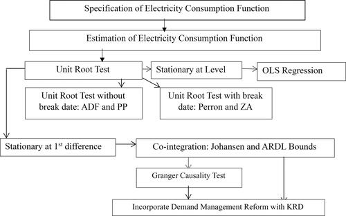
To estimate an electricity consumption function, the first step is to conduct the unit root tests without and with break data (Figure 1). If the variables are stationary at level, we can run the OLS regression directly, since there is no spurious issue in that case. However, if the variables are found to be non-stationary at level, the process is to continue to conduct the unit root tests for all variables at first difference. When variables are stationary at first difference, we can further conduct cointegration tests by Johansen and ARDL approaches. If there is cointegration relationship among variables, the spurious problem will be solved and then the Granger Causality tests and Kink Discontinuity Regression method can be conducted. Based on Chow and Niu (2015), we do not involve any time dummy variables, interaction terms containing time dummy variable, or lagged variables in the unit-root and cointegration tests.

Figure 1. Structural Flow Chart of the Theory and Econometric Methods Utilized. Source: Stata and R software.

4.1. Unit root and cointegration tests

Because standard Granger causality tests should be conducted on stationary time series or cointegration with unit root process, we first test the unit roots of all variables to confirm the stationary properties of each variable. This is achieved by using the Augmented Dickey-Fuller (ADF) test (Dickey and Fuller 1979; Mackinnon, 1996). Expressing the time series variables of lnE_t and lnY_t as X_t, the Augmented Dickey-Fuller (ADF) relationship is: (11) $$X_t={\alpha }_0+{\alpha }_1{X}_{t-1}+{\alpha }_2\mathrm{t}+\sum _{i=1}^l{\beta }_i\Delta X_{t-i}+u_t\mathrm{}$$(11) where Δ is the difference operator, l is the auto-regressive lag length that must be large enough to eliminate possible serial correlation in β_i, ${\alpha }_0$ is a constant, ${\alpha }_1$ is the coefficient of interest, ${\mathrm{\alpha }}_2$ is the coefficient on a time trend, and ${\mathrm{u}}_{\mathrm{t}}$ is the error term.

In addition, Phillips and Perron (1988) propose an alternative (nonparametric) method of controlling for serial correlation when testing for a unit root called the PP test: (12) $$X_t={\alpha }_0+{\alpha }_1\mathrm{t}+{\alpha }_2{X}_{t-1}+u_t\mathrm{}$$(12)

However, when there are any structural breaks in the data, the ADF test is biased towards a spurious acceptance of non-stationarity because of misspecification bias and size distortions. A Perron test allows for a one-time change in structure occurring at time T _B (1< T_B <T, T is the number of observations). The model that is considered in this test is one which allows for an exogenous change in the level of the series： (13) $$X_t={\alpha }_0+{\alpha }_{1}D{T}_t^{\mathrm{*}}+{\alpha }_{2}t+{\alpha }_3{X}_{t-1}+\sum _{i=1}^l{\beta }_i\Delta X_{t-i}+u_t\mathrm{}$$(13) where DT_t* = t -T_B if t > T_B and 0 otherwise. The null hypothesis implies that the data are non-stationary. In this test, the alternative is taken as trend-stationary with a terminal at time T.

The breakpoint choice is correlated with the data utilized and cannot be considered as independent of the data. Zivot and Andrews test (Zivot & Andrews, 1992) addresses this issue by estimating the structural break data endogenously instead of considering an exogenous break date. We estimate the following equations for the Zivot and Andrews test with the endogenous location of the breakpoint λ= T_B / T: (14) $$X_t={\alpha }_0+{\alpha }_{1}D{T}_t^{\mathrm{*}}\left(\mathrm{\lambda }\right)+{\alpha }_{2}t+{\alpha }_3{X}_{t-1}+\sum _{i=1}^l{\beta }_i\Delta X_{t-i}+u_t\mathrm{}$$(14)

The Johansen multivariate cointegration test (Johansen, 1995) takes the following form as below: (15) $$\Delta {\mathit{lnE}}_t=\alpha +\mathrm{\beta }{\mathit{lnE}}_{t-1}+\sum _{i=1}^l{\mathrm{\vartheta }}_i\Delta {\mathit{lnE}}_{t-i}+\mathrm{\phi }{\mathit{lnY}}_t+u_{0t}\mathrm{}$$(15)

Another way to verify the cointegration relationship is to apply an ARDL model (Pesaran et al., 2001), if none of the series are I(2). The ARDL(p, q) model used in this study is expressed as: (16) $$ln{E}_t=a_0+b_{1}t+b_2{\mathit{lnY}}_t+\sum _{i=1}^p{a}_{1i}{\mathit{lnE}}_{t-i}+\sum _{i=0}^{q-1}{a}_{2i}\Delta \left(ln{Y}_{t-i}\right)+u_{1t}$$(16) (17) $$ln{Y}_t=c_0+d_{1}t+d_2{\mathit{lnE}}_t+\sum _{i=1}^p{c}_{1i}ln{Y}_{t-i}+\sum _{i=0}^{q-1}{c}_{2i}\Delta \left(ln{E}_{t-i}\right)+u_{2t}$$(17)

4.2. Granger causality test and kink discontinuity regression

Although the Johansen cointegration test and the ARDL approach to cointegration explore whether the time-series data are cointegrated, they do not reveal the causality directions between ln E_t and ln Y_t. For this purpose, we use the Granger causality (Granger, 1969) as shown in Equations (18)(18) $$ln{E}_t=g_0+\sum _{i=1}^l{g}_i{\mathit{lnY}}_{t-i}+\sum _{i=1}^l{h}_i{\mathit{lnE}}_{t-i}+{\theta }_{1t}\mathrm{}$$(18) and (19)(19) $${\mathit{lnY}}_t=v_0+\sum _{i=1}^l{v}_i{\mathit{lnE}}_{t-i}+\sum _{i=1}^l{w}_i{\mathit{lnY}}_{t-i}+{\theta }_{2t}\mathrm{}$$(19) : (18) $$ln{E}_t=g_0+\sum _{i=1}^l{g}_i{\mathit{lnY}}_{t-i}+\sum _{i=1}^l{h}_i{\mathit{lnE}}_{t-i}+{\theta }_{1t}\mathrm{}$$(18) (19) $${\mathit{lnY}}_t=v_0+\sum _{i=1}^l{v}_i{\mathit{lnE}}_{t-i}+\sum _{i=1}^l{w}_i{\mathit{lnY}}_{t-i}+{\theta }_{2t}\mathrm{}$$(19)

In order to design an experiment to investigate the causal effect of electricity demand management reform program on electricity consumption, we use the KRD (Kink Regression Discontinuity) approach for robustness analysis (Card et al., 2015). The idea of regression discontinuity design is that there is a continuous variable ${\mathit{lnY}}_t$(assignment variable) which determines the treatment variable $D_t$ by a cutoff. The random distribution of samples in a small neighborhood $\left[\delta -\mu ,\delta +\mu \right]$ of ${\mathit{lnE}}_t$ is regarded as “quasi experiment”. By estimating LATE (Local Average Treatment Effect), it is possible to identify whether the dependent variable ($ln{E}_t$) has a cutoff at $ln{Y}_t=\delta ,$ where bandwidth $\mu =\mathit{argmin}\frac{{\sum }_{t=1}^T{[ln{E}_t-E(ln{Y}_t)]}^2}{T}$ and $\mathrm{LATE}=\underset{{\mathit{lnY}}_t\to \delta +}{\lim }\mathrm{E}\left(ln{E}_t\right)-\underset{{\mathit{lnY}}_t\to \delta -}{\lim }\mathrm{E}\left(ln{E}_t\right).$ The null hypothesis of the test is: $H_0\equiv \underset{{\mathit{lnY}}_t\to \delta +}{\lim }ln{E}_t-\underset{{\mathit{lnY}}_t\to \delta -}{\lim }ln{E}_t=0.$ Since the electricity demand management reform occurred from 1985, ${\mathit{lnY}}_{1985}$ is treated as the cutoff. So,$\mathrm{}{D}_t=\{\begin{array}{c}1,\mathit{\text{if}}1985\le t\le 2016\\ 0,if1949\le t\le 1984\end{array}.$

A generalization of electricity consumption function based on Equation (10)(10) $$ln{E}_t={\beta }_0+{\beta }_1{\mathrm{lnY}}_t+{\beta }_2{\mathrm{lnE}}_{t-1}+{\beta }_3{D}_t+{\mathrm{v}}_t\mathrm{}$$(10) allows different trend function for $\mathrm{E}\left[ln{E}_{0t}{\mathit{lnY}}_t\right]$ and $\mathrm{E}\left[ln{E}_{1t}{\mathit{lnY}}_t\right].$ Modeling both of these variables as conditional expectation functions (CEFs) results in Equations (20(20) $$\mathrm{E}\left[ln{E}_{0t}{\mathit{lnY}}_t\right]={\beta }_0+{\beta }_{01}\left({\mathrm{lnY}}_t-{\mathit{lnY}}_{1985}\right)+{\beta }_2{\mathrm{lnE}}_{t-1}\mathrm{}$$(20) and (21)(21) $$\mathrm{E}\left[ln{E}_{1t}{\mathit{lnY}}_t\right]={\beta }_0+{\beta }_3+{\beta }_{11}\left({\mathrm{lnY}}_t-{\mathit{lnY}}_{1985}\right)+{\beta }_2{\mathrm{lnE}}_{t-1}$$(21) : (20) $$\mathrm{E}\left[ln{E}_{0t}{\mathit{lnY}}_t\right]={\beta }_0+{\beta }_{01}\left({\mathrm{lnY}}_t-{\mathit{lnY}}_{1985}\right)+{\beta }_2{\mathrm{lnE}}_{t-1}\mathrm{}$$(20) (21) $$\mathrm{E}\left[ln{E}_{1t}{\mathit{lnY}}_t\right]={\beta }_0+{\beta }_3+{\beta }_{11}\left({\mathrm{lnY}}_t-{\mathit{lnY}}_{1985}\right)+{\beta }_2{\mathrm{lnE}}_{t-1}$$(21)

To derive a regression model that can be used to estimate the causal effect of interest, we use the fact that $D_t$ is a deterministic function of ${\mathrm{lnY}}_t$ to write (22) $$\mathrm{E}\left[ln{E}_t{\mathit{lnY}}_t\right]=\mathrm{E}\left[ln{E}_{0t}{\mathit{lnY}}_t\right]+\left(\mathrm{E}\left[ln{E}_{1t}{\mathit{lnY}}_t\right]-\mathrm{E}\left[ln{E}_{0t}{\mathit{lnY}}_t\right]\right)D_t\mathrm{}$$(22)

Substituting regression for conditional expectations, then we have $$ln{E}_t={\beta }_0+{\beta }_{01}\left({\mathrm{lnY}}_t-{l\mathrm{n}Y}_{1985}\right)+{\beta }_2{\mathrm{lnE}}_{t-1}+{\beta }_3{D}_t+\left({\beta }_{11}-{\beta }_{01}\right)\left({\mathrm{lnY}}_t-{\mathit{lnY}}_{1985}\right)D_t+v_t$$ (23) $$={(\beta }_0-{\beta }_{01}{\mathit{lnY}}_{1985})+{\beta }_{01}{\mathrm{lnY}}_t+{\beta }_2{\mathrm{lnE}}_{t-1}+[-{\left({\beta }_{11}-{\beta }_{01}\right)lnY}_{1985}+{\beta }_3{]D}_t+({\beta }_{11}-{\beta }_{01}){D_t\mathrm{l}\mathrm{nY}}_t+v_t\mathrm{}$$(23)

The electricity consumption function in regression discontinuity reduced form is expressed in Equation (24)(24) $$ln{E}_t={\alpha }_0+{\alpha }_1{\mathrm{lnY}}_t+{\alpha }_2{\mathrm{lnE}}_{t-1}+{\alpha }_3{D}_t+{\alpha }_4{D_t\mathrm{l}\mathrm{nY}}_t+v_t\mathrm{}$$(24) : (24) $$ln{E}_t={\alpha }_0+{\alpha }_1{\mathrm{lnY}}_t+{\alpha }_2{\mathrm{lnE}}_{t-1}+{\alpha }_3{D}_t+{\alpha }_4{D_t\mathrm{l}\mathrm{nY}}_t+v_t\mathrm{}$$(24) where ${\alpha }_0={\beta }_0-{\beta }_{01}{\mathit{lnY}}_{1985},$ ${\alpha }_1={\beta }_{01},$ ${\alpha }_2={\beta }_2,$$\mathrm{}{\alpha }_3=-{({\beta }_{11}-{\beta }_{01})\mathit{lnY}}_{1985}+{\beta }_3,$ and ${\alpha }_4={\beta }_{11}-{\beta }_{01}.$

4.3. Background

With over 2,100 years of history, Guangzhou is a major commercial center in south China (He et al., 2017). Guangzhou is the third largest metropolitan area in China, after Beijing and Shanghai, and the largest city in south central China (Yang et al., 2013). As the capital of Canton Province, it is located within 120 km of both Hong Kong and Macau. Because Guangzhou is adjacent to Hong Kong, which was a colony of the Britain from 1842 to 1997 and is a typical metropolitan market economy, the Chinese central government allowed Guangzhou be an experimental metropolitan in terms of institutional reforms. Thus, Guangzhou has become the commercial and free trade center of south China (Bercht, 2013).

4.4. Data

The Guangzhou Statistical Division provides the most complete and longest duration time series dataset (from 1949 to 2016) among all the metropolitan areas in China.

We utilize this time series data to estimate a metropolitan electricity consumption function. Table 2 lists the variables, their definitions and summary statistics for all variables included in the sample. According to the form of electricity consumption function in Equation (10)(10) $$ln{E}_t={\beta }_0+{\beta }_1{\mathrm{lnY}}_t+{\beta }_2{\mathrm{lnE}}_{t-1}+{\beta }_3{D}_t+{\mathrm{v}}_t\mathrm{}$$(10) , the dependent variable is the natural logarithmic of metropolitan electricity consumption (ln E). The main independent variable is the natural logarithmic of metropolitan economic output (ln Y).

Table 2. Variable definitions and descriptive statistics.

Variable	Definition	Mean	Max	Min	SD	# Obs.
lnE	natural logarithmic of total Electricity Consumption	15.0042	18.2266	10.7938	2.0720	68
lnY	natural logarithmic of (Gross Metropolitan Income*(CPI2016 /CPIt))	25.2587	28.1877	22.5582	1.5437	68

Note: 1) Megawatt Hours is the unit measuring electricity consumption (E); 2) Yuan is the unit for measuring income (Y).

Source: Stata and R software.

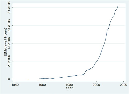
Figures 2 and 3 illustrate the evolution of electricity consumption and gross metropolitan income in Guangzhou throughout the course of the sample period. Both figures show, growth in electricity consumption and income have accelerated since 1985. The growth rates of Y before and after 1985 are 9.9% and 24.7%, while growth rates of E before and after 1985 are 64.51% and 18.34%.

Figure 2. Time Trend of Annual Electricity Consumption in Guangzhou (1949–2016).

Source: Stata and R software.

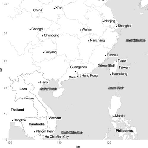
Figure 3. Time Trend of Annual Gross Metropolitan Income in Guangzhou (1949–2016).

Source: Stata and R software.

5. Empirical evidence

5.1. Unit root tests

5.1.1. ADF test and PP test

ADF test and PP test are applied to detect the possible presence of unit roots in ln Y_t and ln E_t. The null hypothesis of unit root can be rejected in favor of the alternative hypothesis of no unit root when the p-value is small (He & Gao 2017). Table 3 indicates that no variable is stationary in their levels since the p-values for each variable are greater than 10%. On the other hand, ln Y_t and ln E_t are stationary process in their first differences because the p-values for ln Y_t are smaller than 1% in both ADF test and PP test. Furthermore, the p-values for ln E_t are smaller than 1% in both tests.

Table 3. ADF and PP unit root tests results.

ADF Test				PP Test
Variable	ADF-test statistics	C,L,T	P-value	Variable	PP-test statistic	C,B,T	P-value
ln Yt	5.0033	(0,0,0)	1.0000	ln Yt	4.4939	(0,1,0)	1.0000
ln Et	–2.3084	(C,0,T)	0.4235	ln Et	–2.2259	(C,8,T)	0.4676
ΔlnYt	–6.3046***	(C,0,0)	0.0000	ΔlnYt	–6.2419***	(C,3,0)	0.0000
ΔlnEt	–5.4752***	(C,2,0)	0.0000	ΔlnEt	–8.2560***	(C,9,T)	0.0000

Note: 1) *** p < 0.01, ** p < 0.05, * p < 0.1; 2) C, L, T, and B represent the constant, and lag length, time trend, bandwidth, respectively.

Source: Stata and R software.

5.1.2. Perron’s modified ADF test and Zivot–Andrews test

The results of Perron’s modified ADF test and Zivot–Andrews test are detailed in Table 4 and Table 5, respectively. They show that non-stationary processes are found in all series at level but variables are found to be stationary at first difference. This confirms that ln Y_t and ln E_t are integrated at I(1).

Table 4. Perron’s modified ADF unit root test results.

Variable	Break Date	T-statistic	C,L,T	10% critical value	5%critical value	1%critical value
lnYt	1988	–3.1969	（0,1,0）	–4.4800	–4.8300	–5.4500
lnEt	1960	–3.7225	（0,0,T）	–4.4800	–4.8300	–5.4500
ΔlnYt	1961	–6.8583***	（0,0,T）	–4.4800	–4.8300	–5.4500
ΔlnEt	1968	–8.8418***	（0,0,T）	–4.4800	–4.8300	–5.4500

Note: 1) *** p < 0.01, ** p < 0.05, * p < 0.1; 2) C, L, and T represent the constant, and lag length, time trend, respectively.

Source: Stata and R software.

Table 5. Zivot-Andrews unit root test results.

Variable	Break Data	T-statistic	C,L,T	10% critical value	5%critical value	1%critical value
lnYt	1961	–3.5614	（0,1,T）	–4.5800	–4.9300	–5.3400
lnEt	1977	–3.7630	（0,1,T）	–4.5800	–4.9300	–5.3400
ΔlnYt	1964	–7.0979*	（C,0,T）	–4.8200	–5.0800	–5.5700
ΔlnEt	1961	–6.9224***	（0,1,T）	–4.8200	–5.0800	–5.5700

Note: 1) *** p < 0.01, ** p < 0.05, * p < 0.1; 2) C, L, and T represent the constant, and lag length, time trend, respectively.

Source: Stata and R software.

5.2. Cointegration tests

Table 6 shows the lag order in Johansen test is one. Based upon unit root test results, integration of variables is of the same order so that we continue to test whether these variables are cointegrated over the sample period (Gao & He, 2017). The Johansen cointegration test in Table 7 shows the trace statistic for non-cointegrating equations (29.0565) is greater than the 5% critical value (20.2618), but not for the at most one cointegrating equation (p-value 0.2781 is greater than 10%). This test rejects the hypothesis of none cointegration and indicates that there is at least one cointegrating equation at the 5% significance level, demonstrating there is a long-run relationship between ln Y_t and ln E_t in Guangzhou.

Table 6. Lag order selection criteria.

Lag	LogL	LR	FPE	AIC	SC	HQ
0	–144.6302	NA	0.3883	4.7300	4.7986	4.7569
1	96.2876	458.5210	0.0001	–2.9125*	−2.7066*	−2.8316*
2	99.6402	6.1644	0.0001	–2.8916	–2.5485	–2.7569
3	105.2899	10.0236	0.0001	−2.9448	–2.4645	–2.7562
4	106.5134	2.0916	0.0001	–2.8552	–2.2377	–2.6128
5	108.1155	2.6358	0.0002	–2.7779	–2.0231	–2.4815
6	109.6122	2.3656	0.0002	–2.6971	–1.8051	–2.3469

Note:1)* indicates lag order selected by the criterion. 2) LR: sequential modified LR test statistic (each test at 5% level).3) FPE: Final prediction error. 4) AIC: Akaike information criterion. 5) SC: Schwarz information criterion. 6) HQ: Hannan-Quinn information criterion.

Source: Stata and R software.

Table 7. Johansen cointegration test results.

Hypothesized Number of Cointegrating equation	Trace Statistic	5%Critical Value	P-value
None***	29.0565	20.2618	0.0024
At most 1	5.0494	9.1645	0.2781

Note: *** p < 0.01, ** p < 0.05, * p < 0.1.

Source: Stata and R software.

The results of the bound test show there exists a long run relationship exists between ln Y_t and ln E_t, because their F-statistic (10.1886) are higher than the upper-bound critical value (5.5800) at the 1% level (Table 8). This implies that the null hypothesis of no cointegration between ln Y_t and ln E_t is rejected, when ln E_t is dependent variable.

Table 8. Bounds test results.

Estimated model	Lag length	F-statistic
f (lnYt/lnEt)	(1,1)	1.2110
f (lnEt/lnYt)	(1,3)	10.1886***
1% critical values	I(0)	I(1)
	4.9400	5.5800

Note: *** p < 0.01, ** p < 0.05, * p < 0.1.

Source: Stata and R software.

5.3. VECM Granger causality analysis

Table 9 reports the Granger causality analysis between lnY_t and lnE_t based on Vector Error Correction Model. Only in the long run, there is a unidirectional Granger causality from lnY_t to lnE_t since the related p-value of ECT_t-1 (0.0048) is less than a 1% level. Moreover, the coefficient of ECT_t-1 is negative and significant. Furthermore, this Granger Causality demonstrates that the evidence from Guangzhou supports the conservation hypothesis. This result is inconsistent with the finding that confirms the Granger Causality running from electricity consumption per capita to economic output per capita in the short run for Guangzhou (He et al., 2017). However, the latter neglects the further discussion on the Granger Causality test for long-run.

Table 9. VECM Granger causality analysis.

Dependent variable	Wald statistics
	Short run		Long run
	ΣΔ lnY t − 1	ΣΔlnE t – 1	ECT t − 1
ΔlnYt	–	1.1692 (0.5573)	0.1186 (0.7305) [0.0103]
ΔlnEt	2.8743 (0.2376)	–	7.9511***(0.0048) [–0.0818]

Note: 1) *** p < 0.01, ** p < 0.05, * p < 0.1; 2) Values in parenthesis are p-values; 3) Values in square brackets are estimated coefficients of ECT_{t − 1}.

Source: Stata and R software.

Moreover, the empirical results in Table 8 just reflect Granger Causality between electricity consumption and economic output, which means a variable ln Y_t is useful in forecasting another variable ln E_t (past values of ln Y_t should contain information that helps predict ln E_t above and beyond the information contained in past values of ln E_t alone) but this does not imply that ln Y_t actually causes ln E_t, in terms of causal inference. To investigate the actual causal effect between electricity consumption and economic output, we need to continue to conduct the causal inference by using KRD approach.

5.4. Regression results incorporating demand management reform using the KRD approach

Because electricity demand management reform in Guangzhou started in 1985, the natural log of real GDP in 1985 (lnY₁₉₈₅) serves as a cutoff to compare electricity consumption prior to and after this date. Therefore, the ln Y_t prior to 1985 are not exposed to reform while ln Y_t in 1985 and all years thereafter are exposed to reform.

Table 10 demonstrates that the local Wald estimator with one bandwidth during the period 1949 to 2016 is significantly positive, which confirms that the natural log of real GDP on 1985 is the cutoff, statistically.

Table 10. Results of local wald estimation.

Period	1949–2016
Cutoff Time	1985
Variable	Coefficient
lwald	0.3694** (0.1702)
N	68

Note: 1) *** p < 0.01, ** p < 0.05, * p < 0.1; 2) Standard errors in parentheses.

Source: Stata and R software.

Table 11 illustrates that the total marginal effects of ln Y_t are significantly positive both prior to 1985 (0.3774) and after 1985 (0.2207 = 0.3774 − 0.1567). This result means that while real GDP increases electricity consumption throughout the entire time-period in Guangzhou, after demand management reform is implemented, its impact is lessened. Since the total marginal effect of ln Y_t represents the income elasticity of electricity demand, we find that electricity consumption under the context of electricity demand management reform increases by 0.2207%, for an 1% change in economic output. Therefore, these results also confirm that there is true causality relationship running from economic output to electricity consumption, which is consistent with the empirical results from Granger Causality Test in Table 9.

Table 11. Results of kink regression discontinuity (dependent variable：lnE_t).

Variable	Coefficient	Robust standard errors
Dt	0.0207	0.0463
lnYt	0.3774 ***	0.1201
Dt * lnYt	–0.1567*	0.0829
lnEt-1	0.8014***	0.0462
Constant	2.6401 ***	0.5982
Adjusted R-squared	0.9955
Bandwidth	2.3461
N	55

Note: 1) *** p < 0.01, ** p < 0.05, * p < 0.1; 2) bandwidth =2.3400.

Source: Stata and R software.

Moreover, since the coefficient of D_t *ln Y_t is negative and statistically significant, after the electricity demand management reform, we conclude that the income elasticity of electricity consumption is lower after reform. we attribute this result to the electricity demand management reform where electricity use has transitioned from a community (public) good to individual (private) good for the residential customers (households). With this reform, it is presumed that the consumers prefer to purchase more energy-efficient appliances (such as compact fluorescent lamp or light emitting diode lamp) as their income increases after reform.

This reform created incentives for households to save electricity (He & Gao 2017). In addition, the regime of peak period rate also constrains commercial and industrial customers’ demand for electricity. Finally, the coefficient of ln E_t-1 is positive and statistically significant (Table 11). This result means that previous electricity consumption habits have a “path dependence” effect on current electricity consumption, because the consumer has formed the habits of consuming electricity.

6. Conclusions

To analyze the nexus between electricity consumption and metropolitan economic output in Guangzhou City, China, we develop a theoretical framework utilizing an inter-temporal, constrained optimization model of societal income with government investment in electricity infrastructure. This model also featured aspects of electricity consumption habits by consumers and electricity demand management reform. A natural experiment design with a kink regression discontinuity method is utilized to evaluate the electricity consumption function after reform. Therefore, a metropolitan electricity consumption function is derived and estimated including GDP, electricity consumption habits, and electricity demand management reform in this study.

Previous studies have explored the nexus between electricity consumption and GDP by only examining empirical relationships without developing an underlying theoretical basis for this relationship (Ghosh, 2002; Ikegami & Wang, 2016; He et al., 2017). Although some empirical researchers have examined Granger causality between electricity consumption and GDP, they do not provide an underlying theoretical explanation for the logic of such a linkage between economic output and electricity consumption.

Based on the theoretical hypotheses developed from our model, the empirical results demonstrate three findings: (1) unidirectional Granger causality running from economic output to electricity consumption, (2) given electricity consumption habits under the context of the electricity demand management reform, an economic output increase of 1% results in the increase of electricity consumption by 0.22% (the income elasticity demand of electricity), and (3), after demand management has been implemented, economic output continues to increase electricity consumption, but at a lower rate than prior to reform. These empirical results imply that the ‘conservation hypothesis’ is upheld over the long-run at the regional level in Guangzhou. In addition, it is instructive that, electricity consumption is the consequence of income growth.

This study is also helpful in balancing the relationship between electricity use and economic reform. Especially, the experience of electricity demand management reform in Guangzhou provides evidence that the “ammeter sole use system” improves the electricity use efficiency (units of electricity use per unit of GDP), because individual households pay for electricity that they actually use.

Different from the conventional research on economic impact of energy use (Collins et al., 2012), the literature on the electricity-growth nexus is dominated by empirical research (Payne, 2010). However, these are variability of causality results, particularly across sample periods, sample sizes, and model specification (Smyth, 2013). Further research in these areas may shed light on regional variations in the functional form of electricity consumption.

Disclosure statement

No potential conflict of interest was reported by the author(s).

Additional information

Funding

This work is financially supported by National Ten Thousand Talent Program [W02070352] and Chinese National Funding of Social Sciences [19FJYB050].

Appendix

This appendix provides a derivation of Equation (10)(10) $$ln{E}_t={\beta }_0+{\beta }_1{\mathrm{lnY}}_t+{\beta }_2{\mathrm{lnE}}_{t-1}+{\beta }_3{D}_t+{\mathrm{v}}_t\mathrm{}$$(10) . This derivation starts with the current Hamiltonian Function from the optimal control problem in Equation (9)(9) $$\genfrac{}{}{0pt}{}{\mathit{Max}}{{\mathrm{G}}_t}\sum _{t=0}^T{\mathrm{Y}}_t{\left(\frac{1}{1+\theta }\right)}^t\mathrm{}$$(9) : (A1) $${\mathcal{H}}_C={\mathrm{A}}_t{\mathrm{K}}_t^a{\left(\mathrm{f}{{\mathrm{\epsilon }}_t\left(D_t\right)\mathrm{F}}_t\right)}^b{\mathrm{L}}_t^d+\left(\frac{1}{1+\theta }\right){\phi }_{t+1}[{\mathrm{A}}_t{\mathrm{K}}_t^a{\left(\mathrm{f}{{\mathrm{\epsilon }}_t\left(D_t\right)\mathrm{F}}_t\right)}^b{\mathrm{L}}_t^d-{\mathrm{C}}_t-G_t-\mathrm{\delta }{\mathrm{K}}_t]+\left(\frac{1}{1+\theta }\right){\tau }_{t+1}({\mathrm{G}}_t-{\text{πF}}_t)\mathrm{}$$(A1) where ${\phi }_t$ is the shadow price of capital at year t and ${\tau }_t$ is the shadow price of stock of electricity infrastructure at year t. The Pontryagin necessary conditions (PNC) are as below: (A2) $$\frac{\partial {\mathcal{H}}_C}{\partial {\mathrm{G}}_t}=-\left(\frac{1}{1+\theta }\right){\phi }_{t+1}+\left(\frac{1}{1+\theta }\right){\tau }_{t+1}=0\mathrm{}$$(A2) (A3) $$\frac{\partial {\mathcal{H}}_C}{\partial F_t}=b{\mathrm{A}}_t{\mathrm{K}}_t^a{({\mathrm{\epsilon }}_t(D_t)\mathrm{f})}^b{\mathrm{F}}_t^{b-1}{\mathrm{L}}_t^d+(\frac{1}{1+\theta }){\phi }_{t+1}b{\mathrm{A}}_t{\mathrm{K}}_t^a{({\mathrm{\epsilon }}_t(D_t)\mathrm{f})}^b{\mathrm{F}}_t^{b-1}{\mathrm{L}}_t^d-(\frac{1}{1+\theta }){\tau }_{t+1}\mathrm{\pi }=-\left[\right(\frac{1}{1+\theta }){\tau }_{t+1}-{\tau }_t]\mathrm{}$$(A3) (A4) $$\frac{\partial {\mathcal{H}}_C}{\partial {\mathrm{K}}_t}=a{\mathrm{A}}_t{\mathrm{K}}_t^{a-1}{\left(\mathrm{f}{{\mathrm{\epsilon }}_t\left(D_t\right)\mathrm{F}}_t\right)}^b{\mathrm{L}}_t^d+\left(\frac{1}{1+\theta }\right){\phi }_{t+1}[a{\mathrm{A}}_t{\mathrm{K}}_t^{a-1}{\left(\mathrm{f}{{\mathrm{\epsilon }}_t\left(D_t\right)\mathrm{F}}_t\right)}^b{\mathrm{L}}_t^d-\mathrm{\delta }]=-\left[\right(\frac{1}{1+\theta }){\phi }_{t+1}-{\phi }_t]\mathrm{}$$(A4)

From (A2), I obtain: (A5) $${\phi }_{t+1}={\tau }_{t+1}\mathrm{}$$(A5)

From (A4), I obtain: $$\left[1+\left(\frac{1}{1+\theta }\right){\phi }_{t+1}\right]a{\mathrm{A}}_t{\mathrm{K}}_t^{a-1}{\left(\mathrm{f}{{\mathrm{\epsilon }}_t\left(D_t\right)\mathrm{F}}_t\right)}^b{\mathrm{L}}_t^d=\left(\frac{1}{1+\theta }\right){\phi }_{t+1}\mathrm{\delta }-\left(\frac{1}{1+\theta }\right){\phi }_{t+1}+{\phi }_t$$

According to the condition that each profit maximizing firm should hire any input up to the point at which the input’s marginal contribution to production is equal to the marginal cost of hiring any input, we assume that there are n units of homogeneous firms in the metropolitan, so ${\mathrm{Y}}_t={\mathrm{ny}}_t$ and ${\mathrm{K}}_t={\mathrm{nk}}_t,$ where ${\mathrm{y}}_t$ and ${\mathrm{k}}_t$ denote each firm’s output and capital input at year t, respectively. Hence, each firm’s marginal productivity of capital should be identical to the interest rate that is supposed to be social discount rate ($\theta =\frac{\partial y_t}{\partial k_t}=\frac{\partial {(ny}_t)}{\partial {(nk}_t)}=\frac{\partial Y_t}{\partial K_t}=a{\mathrm{A}}_t{\mathrm{K}}_t^{a-1}{\left(\mathrm{f}{{\mathrm{\epsilon }}_t\left(D_t\right)\mathrm{F}}_t\right)}^b{\mathrm{L}}_t^d$), so $$\left[\left(\frac{1+\theta }{1+\theta }\right)+\left(\frac{1}{1+\theta }\right){\phi }_{t+1}\right]\theta =\left(\frac{1}{1+\theta }\right){\phi }_{t+1}\mathrm{\delta }-\left(\frac{1}{1+\theta }\right){\phi }_{t+1}+{\phi }_t$$ which reduces to: $${\phi }_{t+1}+\left(-\frac{1+\theta }{\theta -\mathrm{\delta }+1}\right){\phi }_t=-\frac{\theta (1+\theta )}{\theta -\mathrm{\delta }+1}$$

According to the general solution of the first order difference equation, we get (A6) $${\phi }_t=W{[-(-\frac{1+\theta }{1+\theta -\delta }\left)\right]}^t+\frac{-\frac{\theta (1+\theta )}{\theta -\mathrm{\delta }+1}}{1+(-\frac{1+\theta }{\theta -\mathrm{\delta }+1})}\mathrm{}=W{\left(\frac{1+\theta }{1+\theta -\delta }\right)}^t+\mathrm{}\frac{-\theta (1+\theta )}{\theta -\mathrm{\delta }+1-1-\theta }\mathrm{}=W{\left(\frac{1+\theta }{1+\theta -\delta }\right)}^t+\frac{(1+\theta )\theta }{\delta }\mathrm{}\mathrm{}$$(A6) where W is an initial value in the solution of the first order difference equation of ${\phi }_t,$ so it is a constant. Based on (A6), we get (A7) $${\phi }_{t+1}=W{\left(\frac{1+\theta }{1+\theta -\delta }\right)}^{t+1}+\frac{\left(1+\theta \right)\theta }{\delta }=W{\left(\frac{1+\theta }{1+\theta -\delta }\right)}^t\left(\frac{1+\theta }{1+\theta -\delta }\right)+\frac{\left(1+\theta \right)\theta }{\delta }=\left[{\phi }_t-\frac{\left(1+\theta \right)\theta }{\delta }\right]\left(\frac{1+\theta }{1+\theta -\delta }\right)+\frac{\left(1+\theta \right)\theta }{\delta }={\phi }_t\left(\frac{1+\theta }{1+\theta -\delta }\right)-\frac{\left(1+\theta \right)\theta }{\delta }\left(\frac{1+\theta }{1+\theta -\delta }\right)+\frac{\left(1+\theta \right)\theta }{\delta }={\phi }_t\left(\frac{1+\theta }{1+\theta -\delta }\right)+\frac{\left(1+\theta \right)\theta }{\delta }\left[1-\left(\frac{1+\theta }{1+\theta -\delta }\right)\right]={\phi }_t\left(\frac{1+\theta }{1+\theta -\delta }\right)+\frac{\left(1+\theta \right)\theta }{\delta }\frac{\left(1+\theta -\delta -1-\theta \right)}{1+\theta -\delta }={\phi }_t\left(\frac{1+\theta }{1+\theta -\delta }\right)-\frac{\left(1+\theta \right)\theta }{1+\theta -\delta }={(\phi }_t-\theta \left)\right(\frac{1+\theta }{1+\theta -\delta })$$(A7)

Furthermore, from (A3), we obtain $$\left[1+\left(\frac{1}{1+\theta }\right){\phi }_{t+1}\right]b{\mathrm{A}}_t{\mathrm{K}}_t^a{\left({\mathrm{\epsilon }}_t\left(D_t\right)\mathrm{f}\right)}^b{\mathrm{F}}_t^{b-1}{\mathrm{L}}_t^d=\left(\frac{1}{1+\theta }\right){\tau }_{t+1}\mathrm{\pi }-\left(\frac{1}{1+\theta }\right){\tau }_{t+1}+{\tau }_t$$

This equation can be solved for F_t such that: (A8) $$F_t=\frac{\left({1+\theta +\phi }_{t+1}\right)b}{{\tau }_{t+1}\left(\pi -1\right)+(1+\theta ){\tau }_t}{Y}_t\mathrm{}=\frac{\left({1+\theta +\phi }_{t+1}\right)b}{{\phi }_{t+1}\left(\pi -1\right)+(1+\theta ){\phi }_t}{Y}_t\mathrm{}$$(A8)

Plug (A6), (A7) into (A8), we obtain: (A9) $$F_t=\frac{[1+\theta +{(\phi }_t-\theta )\left(\frac{1+\theta }{1+\theta -\delta }\right)]b}{{(\phi }_t-\theta \left)\right(\frac{1+\theta }{1+\theta -\delta }\left)\right(\pi -1)+(1+\theta ){\phi }_t}{Y}_t=\frac{\frac{\left(1+\theta \right)\left(1+\theta -\delta \right)+{\left(1+\theta \right)(\phi }_t-\theta )}{1+\theta -\delta }}{\frac{\left(\pi -1\right){(\phi }_t-\theta \left)\right(1+\theta )}{1+\theta -\delta }+\frac{(1+\theta -\delta )(1+\theta ){\phi }_t}{1+\theta -\delta }}b{Y}_t=\frac{\left(1+\theta \right)\left(1+\theta -\delta {+\phi }_t-\theta \right)}{\left(1+\theta \right)\left[{\phi }_t\left(\pi -1+1+\theta -\delta \right)-\theta \left(\pi -1\right)\right]}b{Y}_t=\frac{\left(1-\delta {+\phi }_t\right)}{{\phi }_t\left(\pi +\theta -\delta \right)+\theta \left(1-\pi \right)}b{Y}_t\mathrm{}=\frac{[1-\delta +W{\left(\frac{1+\theta }{1+\theta -\delta }\right)}^t+\frac{\left(1+\theta \right)\theta }{\delta }]b}{[W{\left(\frac{1+\theta }{1+\theta -\delta }\right)}^t+\frac{(1+\theta )\theta }{\delta }]\left(\pi +\theta -\delta \right)+\theta \left(1-\pi \right)}{Y}_t\mathrm{}$$(A9)

According to the transfer relationship between electricity capacity and electricity consumption${\mathrm{E}}_t={\mathrm{fF}}_t{\mathrm{\epsilon }}_t\left(D_t\right),$ plug (A9) into it, we obtain the optimal electricity function (A10) $$E_t=\frac{[W{\left(\frac{1+\theta }{1+\theta -\delta }\right)}^t+\frac{\left(1+\theta \right)\theta }{\delta }+1-\delta ]b}{[W{\left(\frac{1+\theta }{1+\theta -\delta }\right)}^t+\frac{(1+\theta )\theta }{\delta }]\left(\pi +\theta -\delta \right)+\theta \left(1-\pi \right)}f{\mathrm{\epsilon }}_t\left(D_t\right)Y_t\mathrm{}$$(A10)

If we let ${\beta }_t=\frac{[W{\left(\frac{1+\theta }{1+\theta -\delta }\right)}^t+\frac{\left(1+\theta \right)\theta }{\delta }+1-\delta ]bf{\mathrm{\epsilon }}_t\left(D_t\right)}{[W{(\frac{1+\theta }{1+\theta -\delta })}^t+\frac{(1+\theta )\theta }{\delta }]\left(\pi +\theta -\delta \right)+\theta \left(1-\pi \right)},$ then the metropolitan electricity consumption function can be expressed as:$E_t={\beta }_t{Y}_t.$ Therefore, (A11) $$ln{E}_t=ln{\beta }_t+ln{Y}_t=\ln \left[W{\left(\frac{1+\theta }{1+\theta -\delta }\right)}^t+\frac{\left(1+\theta \right)\theta }{\delta }+1-\delta \right]+\ln \left(bf\right)\mathrm{}+\mathrm{}\ln \left({\mathrm{\epsilon }}_t\left(D_t\right)\right)-\ln \{\left[W{\left(\frac{1+\theta }{1+\theta -\delta }\right)}^t+\frac{\left(1+\theta \right)\theta }{\delta }\right]\left(\pi +\theta -\delta \right)+\theta \left(1-\pi \right)\}+ln{Y}_t=\ln \left[W{\left(\frac{1+\theta }{1+\theta -\delta }\right)}^t+\frac{\left(1+\theta \right)\theta }{\delta }+1-\delta \right]-\ln \{\left[W{\left(\frac{1+\theta }{1+\theta -\delta }\right)}^t+\frac{\left(1+\theta \right)\theta }{\delta }\right]\left(\pi +\theta -\delta \right)+\theta (1-\pi \left)\right\}+\ln \left(bf\right)\mathrm{}+ln{Y}_t+\mathrm{}\ln \left({\mathrm{\epsilon }}_t\left(D_t\right)\right)=B_0+B_1+B_2\mathrm{l}\mathrm{n}{\mathrm{Y}}_t^e+{ϵ}_t$$(A11) where$\mathrm{}{B}_1=\ln \left(bf\right)$ and ${ϵ}_t=\ln \left({\epsilon }_t\left(D_t\right)\right).$ $B_2\mathrm{l}\mathrm{n}{\mathrm{Y}}_t^e=ln{Y}_t$ means that expected income is assumed to be linearly associated with current income ($\ln {\mathrm{Y}}_t^e=\frac{ln{Y}_t}{B_2}$), which is supported by the evidence from Campbell and Mankiw (1990).

Since $$\frac{\left(1+\theta \right)\theta }{\delta }+1-\delta >0$$

, and then $$\ln \{W{\left(\frac{1+\theta }{1+\theta -\delta }\right)}^t+[\frac{\left(1+\theta \right)\theta }{\delta }+1-\delta ]\}>\ln \left[W{\left(\frac{1+\theta }{1+\theta -\delta }\right)}^{\mathrm{t}}\right]=\mathit{lnW}+ln{\left(\frac{1+\theta }{1+\theta -\delta }\right)}^t=\mathit{lnW}+\mathit{tln}\left(\frac{1+\theta }{1+\theta -\delta }\right)$$

. So, there should be a positive constant z1 satisfying that $$z_1=\ln \{W{\left(\frac{1+\theta }{1+\theta -\delta }\right)}^t+[\frac{\left(1+\theta \right)\theta }{\delta }+1-\delta ]\}-[\mathit{lnW}+\mathit{tln}\left(\frac{1+\theta }{1+\theta -\delta }\right)]$$

Therefore, $$\ln \{W{\left(\frac{1+\theta }{1+\theta -\delta }\right)}^t+[\frac{\left(1+\theta \right)\theta }{\delta }+1-\delta ]\}=\mathit{lnW}+\mathit{tln}\left(\frac{1+\theta }{1+\theta -\delta }\right)+z_1$$

Similarly, $\ln \{\left[W{\left(\frac{1+\theta }{1+\theta -\delta }\right)}^t+\frac{\left(1+\theta \right)\theta }{\delta }\right]\left(\pi +\theta -\delta \right)+\theta \left(1-\pi \right)\}=\ln \{W\left(\pi +\theta -\delta \right){\left(\frac{1+\theta }{1+\theta -\delta }\right)}^t+[\frac{\left(1+\theta \right)\theta \left(\pi +\theta -\delta \right)}{\delta }+\theta (1-\pi \left)\right]\}=\ln [W\left(\pi +\theta -\delta \right)]+\mathit{tln}(\frac{1+\theta }{1+\theta -\delta })+z_2,$ where $z_2=\ln \{\left[W{\left(\frac{1+\theta }{1+\theta -\delta }\right)}^t+\frac{\left(1+\theta \right)\theta }{\delta }\right]\left(\pi +\theta -\delta \right)+\theta \left(1-\pi \right)\}-\{\ln [W\left(\pi +\theta -\delta \right)]+\mathit{tln}(\frac{1+\theta }{1+\theta -\delta }\left)\right\}.$

Therefore, $$\ln \left[W{\left(\frac{1+\theta }{1+\theta -\delta }\right)}^t+\frac{\left(1+\theta \right)\theta }{\delta }+1-\delta \right]-\ln \{\left[W{\left(\frac{1+\theta }{1+\theta -\delta }\right)}^t+\frac{\left(1+\theta \right)\theta }{\delta }\right]\left(\pi +\theta -\delta \right)+\theta \left(1-\pi \right)\}=[\mathit{lnW}+\mathit{tln}\left(\frac{1+\theta }{1+\theta -\delta }\right)+z_1]-\{\ln \left[W\left(\pi +\theta -\delta \right)\right]+\mathit{tln}\left(\frac{1+\theta }{1+\theta -\delta }\right)+z_2\}=\mathit{lnW}+z_1-\ln \left[W\left(\pi +\theta -\delta \right)\right]-z_2=z_1-z_2-\ln \left(\pi +\theta -\delta \right)=B_0$$

In terms of Equation (A11)(A11) $$ln{E}_t=ln{\beta }_t+ln{Y}_t=\ln \left[W{\left(\frac{1+\theta }{1+\theta -\delta }\right)}^t+\frac{\left(1+\theta \right)\theta }{\delta }+1-\delta \right]+\ln \left(bf\right)\mathrm{}+\mathrm{}\ln \left({\mathrm{\epsilon }}_t\left(D_t\right)\right)-\ln \{\left[W{\left(\frac{1+\theta }{1+\theta -\delta }\right)}^t+\frac{\left(1+\theta \right)\theta }{\delta }\right]\left(\pi +\theta -\delta \right)+\theta \left(1-\pi \right)\}+ln{Y}_t=\ln \left[W{\left(\frac{1+\theta }{1+\theta -\delta }\right)}^t+\frac{\left(1+\theta \right)\theta }{\delta }+1-\delta \right]-\ln \{\left[W{\left(\frac{1+\theta }{1+\theta -\delta }\right)}^t+\frac{\left(1+\theta \right)\theta }{\delta }\right]\left(\pi +\theta -\delta \right)+\theta (1-\pi \left)\right\}+\ln \left(bf\right)\mathrm{}+ln{Y}_t+\mathrm{}\ln \left({\mathrm{\epsilon }}_t\left(D_t\right)\right)=B_0+B_1+B_2\mathrm{l}\mathrm{n}{\mathrm{Y}}_t^e+{ϵ}_t$$(A11) , current electricity consumption is dependent on indirectly determined by consumers’ income to be spent on purchasing appliance in the future. The values of durable goods are relatively higher and the life span of them is longer than that of nondurable goods. Therefore, we use the expectation of income to purchase durable items that use electricity (Modigliani, 1985). Appliances are durable goods, so consumers must utilize electricity to create consumption. Therefore, the appliance consumption is determined by consumer’s future income and then electricity consumption is indirectly associated to consumer’s expectation income. Based on this logic, if we estimate electricity consumption function, and then we suppose the natural log of metropolitan electricity consumption at year t ${\mathit{lnE}}_t$ can also the linear function of expectation of the natural log of real GDP $(\ln {\mathrm{Y}}_t^e),$ time trend t and error term$\mathrm{}{ϵ}_t.$

Furthermore, according to the theory of rational expectation (Muth, 1961), let $\ln {\mathrm{Y}}_t^e$ be the expectation value composed of natural log of current real GDP (${\mathrm{lnY}}_t$) and expectation of natural log of previous real GDP ($\ln {\mathrm{Y}}_{t-1}^e$): (A12) $${\mathrm{lnY}}_t^e={(1-b)ln\mathrm{Y}}_t+b{\mathrm{lnY}}_{t-1}^e\mathrm{}$$(A12)

So, plug (A12) into (A11), electricity consumption function can be express like this: (A13) $$ln{E}_t=B_0+B_1+B_2[{\left(1-b\right)ln\mathrm{Y}}_t+b{\mathrm{lnY}}_{t-1}^e]+{ϵ}_t\mathrm{}$$(A13)

According to Equation (A12)(A12) $${\mathrm{lnY}}_t^e={(1-b)ln\mathrm{Y}}_t+b{\mathrm{lnY}}_{t-1}^e\mathrm{}$$(A12) , we obtain: (A14) $${\mathrm{lnY}}_{t-1}^e={(1-b)ln\mathrm{Y}}_{t-1}+b{\mathrm{lnY}}_{t-2}^e\mathrm{}$$(A14) (A15) $${\mathrm{lnY}}_{t-2}^e={(1-b)ln\mathrm{Y}}_{t-2}+b{\mathrm{lnY}}_{t-3}^e$$(A15)

Plug (A14) and (A15) into (A12): (A16) $${\mathrm{lnY}}_t^e={\left(1-b\right)ln\mathrm{Y}}_t+b\left[{\left(1-b\right)ln\mathrm{Y}}_{t-1}+b{\mathrm{lnY}}_{t-2}^e\right]={\left(1-b\right)ln\mathrm{Y}}_t+b{\left(1-b\right)ln\mathrm{Y}}_{t-1}+b^2\left[{\left(1-b\right)ln\mathrm{Y}}_{t-2}+b{\mathrm{lnY}}_{t-3}^e\right]={\left(1-b\right)\mathrm{l}\mathrm{nY}}_t+{\left(1-b\right)b\mathrm{lnY}}_{t-1}+{\left(1-b\right)b^2\mathrm{l}\mathrm{nY}}_{t-2}+b^3{\mathrm{lnY}}_{t-3}^e\mathrm{}={\left(1-b\right)(\mathrm{lnY}}_t+b{\mathrm{lnY}}_{t-1}+b^2{\mathrm{lnY}}_{t-2}+\cdots )$$(A16)

Plug (A16) into (A13): (A17) $$ln{E}_t=B_0+B_1+B_2\left[{\left(1-b\right)ln\mathrm{Y}}_t+b{\mathrm{lnY}}_{t-1}^e\right]+{ϵ}_t=B_0+B_1+B_2{\left(1-b\right)ln\mathrm{Y}}_t+B_{2}b{\mathrm{lnY}}_{t-1}^e+{ϵ}_t=B_0+B_1+B_2{\left(1-b\right)ln\mathrm{Y}}_t+B_{2}b{\left[\right(1-b\left)\right(\mathrm{lnY}}_{t-1}+b{\mathrm{lnY}}_{t-2}+b^2{\mathrm{lnY}}_{t-3}+\cdots \left)\right]+{ϵ}_t=B_0+B_1+B_2{\left(1-b\right)(\mathrm{lnY}}_t+b{\mathrm{lnY}}_{t-1}+b^{2}ln{\mathrm{Y}}_{t-2}+b^{3}ln{\mathrm{Y}}_{t-3}+\cdots )+{ϵ}_t\mathrm{}$$(A17)

So, we obtain: (A18) $$ln{E}_{t-1}=B_0+B_1+B_2{\left(1-b\right)(\mathrm{lnY}}_{t-1}+b{\mathrm{lnY}}_{t-2}+b^2{\mathrm{lnY}}_{t-3}+b^{3}ln{\mathrm{Y}}_{t-4}+\cdots )+{ϵ}_{t-1}\mathrm{}$$(A18)

Let (A17)-b*(A18): $$ln{E}_t-\mathit{bln}{E}_{t-1}$$ (A19) $$=B_0+B_1-\mathrm{b}{B}_0-b{B}_1+B_2{\left(1-b\right)(\mathrm{lnY}}_t+b{\mathrm{lnY}}_{t-1}+b^2{\mathrm{lnY}}_{t-2}+b^{3}ln{\mathrm{Y}}_{t-3}+\cdots )-B_2{\left(1-b\right)(\mathrm{blnY}}_{t-1}+b^2{\mathrm{lnY}}_{t-2}+b^{3}ln{\mathrm{Y}}_{t-3}+b^{4}ln{\mathrm{Y}}_{t-4}+\cdots )+{ϵ}_t\mathrm{}-b{ϵ}_{t-1}\mathrm{}=B_0\left(1-b\right)+B_1(1-b)+B_2{\left(1-b\right)\left[\right(\mathrm{lnY}}_t+b{\mathrm{lnY}}_{t-1}+b^2{\mathrm{lnY}}_{t-2}+b^{3}ln{\mathrm{Y}}_{t-3}+b^{4}ln{\mathrm{Y}}_{t-4}+\cdots )-{(\mathrm{blnY}}_{t-1}+b^2{\mathrm{lnY}}_{t-2}+b^3{\mathrm{lnY}}_{t-3}+b^{4}ln{\mathrm{Y}}_{t-4}+\cdots )]+({ϵ}_t\mathrm{}–b{ϵ}_{t-1})=[\left(B_0+B_1\right)\left(1-b\right)]+B_2{\left(1-b\right)\mathrm{l}\mathrm{nY}}_t+({ϵ}_t\mathrm{}–b{ϵ}_{t-1})$$(A19)

Hence, from (A19), the reduced form of metropolitan electricity consumption is (A20) $$ln{E}_t=\left[\left(B_0+B_1\right)\left(1-b\right)\right]+B_2{\left(1-b\right)\mathrm{l}\mathrm{nY}}_t+\mathit{bln}{E}_{t-1}+\left({ϵ}_t\mathrm{}–b{ϵ}_{t-1}\right)={\beta }_0+{\beta }_1{\mathrm{lnY}}_t+{\beta }_2{\mathrm{lnE}}_{t-1}+e_t\mathrm{}$$(A20) where ${\beta }_0=(B_0+B_1)(1-b),$ ${\beta }_1=B_2(1-\mathrm{b}),$ ${\beta }_2=b$ and $e_t={ϵ}_t–b{ϵ}_{t-1}=h({\mathrm{\epsilon }}_t\left(D_t\right)).$ Equation (A20)(A20) $$ln{E}_t=\left[\left(B_0+B_1\right)\left(1-b\right)\right]+B_2{\left(1-b\right)\mathrm{l}\mathrm{nY}}_t+\mathit{bln}{E}_{t-1}+\left({ϵ}_t\mathrm{}–b{ϵ}_{t-1}\right)={\beta }_0+{\beta }_1{\mathrm{lnY}}_t+{\beta }_2{\mathrm{lnE}}_{t-1}+e_t\mathrm{}$$(A20) means that the current electricity consumption is determined by the previous electricity consumption and the current real GDP, and other factors in error term. Here, previous electricity consumption can be considered as the electricity consumption habits.

Finally, if we assume$\mathrm{}{e}_t=h({\mathrm{\epsilon }}_t\left(D_t\right))={\beta }_3{D}_t+v_t,$ where $v_t$ denotes the unobservable factors excluding electricity demand management reform, then the electricity consumption function is as below: (A21) $$ln{E}_t={\beta }_0+{\beta }_1{\mathrm{lnY}}_t+{\beta }_2{\mathrm{lnE}}_{t-1}+{\beta }_3{D}_t+v_t\mathrm{}$$(A21)

References

- Acaravci, A. (2010). The causal relationship between electricity consumption and GDP in Turkey: evidence from ARDL bounds testing approach. Economic Research-Ekonomska Istraživanja, 23(2), 34–43. https://doi.org/https://doi.org/10.1080/1331677X.2010.11517410
- Akinlo, A. E. (2009). Electricity consumption and economic growth in Nigeria: evidence from cointegration and co-feature analysis. Journal of Policy Modeling, 31(5), 681–693. https://doi.org/https://doi.org/10.1016/j.jpolmod.2009.03.004
- Al-Mulali, U., Fereidouni, H. G., & Lee, J. Y. M. (2014). Electricity consumption from renewable and non-renewable sources and economic growth: evidence from Latin American countries. Renewable and Sustainable Energy Reviews, 30(1), 290–298. https://doi.org/https://doi.org/10.1016/j.rser.2013.10.006
- Altinay, G., & Karagol, E. (2005). Electricity consumption and economic growth: evidence from Turkey. Energy Economics, 27(6), 849–856. https://doi.org/https://doi.org/10.1016/j.eneco.2005.07.002
- Baxter, J. L., & Moosa, I. A. (1996). The consumption function: a basic needs hypothesis. Journal of Economic Behavior & Organization, 31(1), 85–100. https://doi.org/https://doi.org/10.1016/S0167-2681(96)00866-9
- Bercht, A. L. (2013). Glurbanization of the chinese megacity guangzhou-image-building and city development through entrepreneurial governance. Geographica Helvetica, 68(2), 129–138. https://doi.org/https://doi.org/10.5194/gh-68-129-2013
- Bildirici, M. E., & Kayikçi, F. (2012). Economic growth and electricity consumption in former Soviet republics. Energy Economics, 34(3), 747–753. https://doi.org/https://doi.org/10.1016/j.eneco.2012.02.010
- Campbell, J., & Mankiw, G. (1990). Permanent income,current income,and consumption. Journal of Business & Economic Statistics, 8(3), 265–279.
- Card, D., Pei, Z., Lee, D., & Weber, A. (2015). Inference on causal effects in a generalized regression kink design. Econometrica, 83(6), 2453–2483. https://doi.org/https://doi.org/10.3982/ECTA11224
- Chen, S. T., Kuo, H. I., & Chen, C. C. (2007). The relationship between GDP and electricity consumption in 10 Asian countries. Energy Policy, 35(4), 2611–2621. https://doi.org/https://doi.org/10.1016/j.enpol.2006.10.001
- Chow, G. C., & Niu, L. (2015). Housing prices in urban China as determined by demand and supply. Pacific Economic Review, 20(1), 1–16. https://doi.org/https://doi.org/10.1111/1468-0106.12080
- Ciarreta, A., & Zarraga, A. (2010). Economic growth-electricity consumption causality in 12 European countries: a dynamic panel data approach. Energy Policy, 38(7), 3790–3796. https://doi.org/https://doi.org/10.1016/j.enpol.2010.02.058
- Collins, A. R., Hansen, E., & Hendryx, M. (2012). Wind versus coal: comparing the local economic impacts of energy resource development in Appalachia. Energy Policy, 50(2), 551–561. https://doi.org/https://doi.org/10.1016/j.enpol.2012.08.001
- Dickey, D., & Fuller, W. (1979). Distribution of the estimators for autoregressive time series with a unit root. Journal of the American Statistical Association, 74(6), 427–431.
- Friedman, M. (1957). A Theory of the Consumption Function. Princeton University Press.
- Gao, S., & He, Y. (2017). The effect of urbanization and economic performance on metropolitan water consumption: theoretic model and evidence from Guangzhou of China. Applied Economics and Finance, 4(2), 163–171. https://doi.org/https://doi.org/10.11114/aef.v4i2.2076
- Ghosh, S. (2002). Electricity consumption and economic growth in India. Energy Policy, 30(2), 125–129. https://doi.org/https://doi.org/10.1016/S0301-4215(01)00078-7
- Gorman, A. W. M. (1964). Professor Friedman’s consumption function and the theory of choice. Econometrica, 32(1/2), 189–197. https://doi.org/https://doi.org/10.2307/1913744
- Granger, C. W. J. (1969). Investigating causal relations by econometric models and cross-spectral methods. Econometrica, 37(3), 424–4438. [Database] https://doi.org/https://doi.org/10.2307/1912791
- Griliches, Z., Maddala, G. S., Lucas, R., & Wallace, N. (1962). Notes on estimated aggregate quarterly consumption functions. Econometrica, 30(3), 491–500. https://doi.org/https://doi.org/10.2307/1909892
- Hamdi, H., Sbia, R., & Shahbaz, M. (2014). The nexus between electricity consumption and economic growth in Bahrain. Economic Modelling, 38(2), 227–237. https://doi.org/https://doi.org/10.1016/j.econmod.2013.12.012
- He, Y., Fullerton, T. M., & Walke, A. G. (2017). Electricity consumption and metropolitan economic performance in Guangzhou: 1950–2013. Energy Economics, 63, 154–160. https://doi.org/https://doi.org/10.1016/j.eneco.2017.02.002
- He, Y., & Gao, S. (2017). Coasian theorem, public domain, and property rights protection. Asian Economic and Financial Review, 7(5), 470–485. https://doi.org/https://doi.org/10.18488/journal.aefr/2017.7.5/102.5.470.485
- He, Y., & Gao, S. (2017). Gas consumption and metropolitan economic performance: models and empirical studies from Guangzhou. China. International Journal of Energy Economics and Policy, 7(2), 121–126.
- Ho, C. Y., & Siu, K. W. (2007). A dynamic equilibrium of electricity consumption and GDP in Hong Kong: An empirical investigation. Energy Policy, 35(4), 2507–2513. https://doi.org/https://doi.org/10.1016/j.enpol.2006.09.018
- Huang, H., Du, Z., & He, Y. (2018). The effect of population expansion on energy consumption in canton of China: A simulation from computable general equilibrium approach. International Journal of E Ngineering Sciences & M Anagement Research, 5(1), 19–26.
- Ikegami, M., & Wang, Z. (2016). The long-run causal relationship between electricity consumption and real GDP: Evidence from Japan and Germany. Journal of Policy Modeling, 38(5), 767–784. https://doi.org/https://doi.org/10.1016/j.jpolmod.2016.10.007
- Jamil, F., & Ahmad, E. (2010). The relationship between electricity consumption, electricity prices and GDP in Pakistan. Energy Policy, 38(10), 6016–6025. https://doi.org/https://doi.org/10.1016/j.enpol.2010.05.057
- Johansen, S. (1995). A statistical analysis of cointegratio for I(2) variable. Econometric Theory, 11(1), 25–59. https://doi.org/https://doi.org/10.1017/S0266466600009026
- Jumbe, C. B. L. (2004). Cointegration and causality between electricity consumption and GDP: Empirical evidence from Malawi. Energy Economics, 26(1), 61–68. https://doi.org/https://doi.org/10.1016/S0140-9883(03)00058-6
- Kónya, L., & Abdullaev, B. (2018). An attempt to restore Wagner’s Law of increasing state activity. Empirical Economics, 55(4), 1569–1583. https://doi.org/https://doi.org/10.1007/s00181-017-1339-x
- Mackinnon, J. G. (1996). Numerical distribution functions for unit root. Journal of Applied Econometrics, 11(6), 601–618. https://doi.org/https://doi.org/10.1002/(SICI)1099-1255(199611)11:6<601::AID-JAE417>3.0.CO;2-T
- Modigliani, F. (1985). Life cycle, individual thrift, and the wealth of nations. The American Economic Review, 76(3), 297–313.
- Muth, J. F. (1961). Rational expectations and the theory of price movements. Econometrica, 29(3), 315–335. https://doi.org/https://doi.org/10.2307/1909635
- Narayan, P. K., Nielsen, I., & Smyth, R. (2008). Panel data, cointegration, causality and Wagner’s law: empirical evidence from Chinese Provinces. China Economic Review, 19(2), 297–307. https://doi.org/https://doi.org/10.1016/j.chieco.2006.11.004
- Narayan, P. K., & Prasad, A. (2008). Electricity consumption-real GDP causality nexus: evidence from a bootstrapped causality test for 30 OECD countries. Energy Policy, 36(2), 910–918. [Database] https://doi.org/https://doi.org/10.1016/j.enpol.2007.10.017
- Narayan, P. K., & Singh, B. (2007). The electricity consumption and GDP nexus for the Fiji Islands. Energy Economics, 29(6), 1141–1150.
- Odhiambo, N. M. (2009). Electricity consumption and economic growth in South Africa: A trivariate causality test. Energy Economics, 31(5), 635–640. https://doi.org/https://doi.org/10.1016/j.eneco.2009.01.005
- Ouédraogo, I. M. (2010). Electricity consumption and economic growth in Burkina Faso: A cointegration analysis. Energy Economics, 32(3), 524–531. https://doi.org/https://doi.org/10.1016/j.eneco.2009.08.011
- Ozturk, I., & Acaravci, A. (2011). Electricity consumption and real GDP causality nexus: evidence from ARDL bounds testing approach for 11 MENA countries. Applied Energy, 88(8), 2885–2892. https://doi.org/https://doi.org/10.1016/j.apenergy.2011.01.065
- Payne, J. E. (2010). A survey of the electricity consumption-growth literature. Applied Energy, 87(3), 723–731. https://doi.org/https://doi.org/10.1016/j.apenergy.2009.06.034
- Pesaran, M. H., Shin, Y., & Smith, R. J. (2001). Bounds testing approaches to the analysis of level relationships. Journal of Applied Econometrics, 16(3), 289–326. https://doi.org/https://doi.org/10.1002/jae.616
- Phillips, P. C. B., & Perron, P. (1988). Testing for a unit root in time series regression. Biometrika, 75(2), 335–346. https://doi.org/https://doi.org/10.1093/biomet/75.2.335
- Pollitt, M. G., Yang, C., & Chen, H. (2017). Reforming the Chinese Electricity Supply Sector: Lessons from International Experience (No. 1704). Cambridge Working Paper in Economics.
- Shahbaz, M., & Lean, H. H. (2012). The dynamics of electricity consumption and economic growth: a revisit study of their causality in Pakistan. Energy, 39(1), 146–153. https://doi.org/https://doi.org/10.1016/j.energy.2012.01.048
- Shahbaz, M., Tang, C. F., & Shahbaz Shabbir, M. (2011). Electricity consumption and economic growth nexus in Portugal using cointegration and causality approaches. Energy Policy, 39(6), 3529–3536. https://doi.org/https://doi.org/10.1016/j.enpol.2011.03.052
- Shiu, A., & Lam, P. L. (2004). Electricity consumption and economic growth in China. Energy Policy, 32(1), 47–54. [Database] https://doi.org/https://doi.org/10.1016/S0301-4215(02)00250-1
- Smyth, R. (2013). Are fluctuations in energy variables permanent or transitory? a survey of the literature on the integration properties of energy consumption and production. Applied Energy, 104(6), 371–378. https://doi.org/https://doi.org/10.1016/j.apenergy.2012.10.069
- Spiro, A. (1962). Wealth and the consumption function. Journal of Political Economy, 70(4), 339–354. https://doi.org/https://doi.org/10.1086/258662
- Stern, D. I., Burkes, P. J., Bruns, S. B., & Burke, P. J. (2018). The impact of electricity on economic development: a macroeconomic perspective. International Review of Environmental and Resource Economics, 12(1), 85–127.
- Tang, C. F. (2008). A re-examination of the relationship between electricity consumption and economic growth in Malaysia. Energy Policy, 36(8), 3067–3075. https://doi.org/https://doi.org/10.1016/j.enpol.2008.04.026
- Thompson, E. A. (1967). Intertemporal utility functions and the long-run consumption function. Econometrica, 35(2), 356–361. https://doi.org/https://doi.org/10.2307/1909117
- Xu, C. (2011). The fundamental institutions of China’s reforms and development. Journal of Economic Literature, 49(4), 1076–1151. https://doi.org/https://doi.org/10.1257/jel.49.4.1076
- Yang, C. L., Lin, H. P., & Chang, C. H. (2010). Linear and nonlinear causality between sectoral electricity consumption and economic growth: evidence from Taiwan. Energy Policy, 38(11), 6570–6573.
- Yang, J., Liu, H., & Leatham, D. J. (2013). The multi-market analysis of a housing price transmission model. Applied Economics, 45(27), 3810–3819. https://doi.org/https://doi.org/10.1080/00036846.2012.734595
- Yoo, S.-H. (2005). Electricity consumption and economic growth: evidence from Korea. Energy Policy, 33(12), 1627–1632. https://doi.org/https://doi.org/10.1016/j.enpol.2004.02.002
- Yoo, S. H. (2006). The causal relationship between electricity consumption and economic growth in the ASEAN countries. Energy Policy, 34(18), 3573–3582. https://doi.org/https://doi.org/10.1016/j.enpol.2005.07.011
- Yuan, J., Zhao, C., Yu, S., & Hu, Z. (2007). Electricity consumption and economic growth in China: cointegration and co-feature analysis. Energy Economics, 29(6), 1179–1191. https://doi.org/https://doi.org/10.1016/j.eneco.2006.09.005
- Zellner, A. (1957). The short-run consumption function. Econometrica, 25(4), 552–1275. https://doi.org/https://doi.org/10.2307/1905383
- Zellner, B. Y. A., & Geisel, M. S. (1970). Analysis of distributed lag models with applications to consumption function estimation. Econometrica, 38(6), 865–888. https://doi.org/https://doi.org/10.2307/1909697
- Zivot, E., & Andrews, D. W. K. (1992). Further evidence oil-price shock, hypothesis on and the the great crash, unit-root the eric. Journal of Business & Economic Statistics, 10(3), 251–270.