High-speed rail to prosperity? Assessing the role of transportation improvement in the urban economy

Abstract

Investigate the impact of high-speed rail (HSR) on local economy is of great importance and interest to policy makers and scholars. Though there is a big body of literature in this area, the estimates of such impact are inconsistent or even contradictory. The empirical evidence remains problematic for several reasons: endogenous route placement; omitted variable bias; heterogeneity across different regions; various confounding factors. In this paper, we assess this impact by constructing the appropriate counterfactual in the absence of HSR services with similar GDP level and GDP trend before the debut of HSR services. The control group forms a good fit for the treatment group, and the economic performance of the control group was even slightly stronger than that of the treatment group before 2007. Using the DID method, we find the HSR network promoted local GDP by approximately 3.3 percentage points. The introduction of HSR service helped cities attract more industrial enterprises and achieve more industrial output, but its effect on the service sector was not pronounced. Our results are robust to different sample selection procedures, to the dynamic analyses, to different empirical strategies. Our study thus provides new and solid empirical support to the argument that HSR benefits local economic development.

Keywords:

• HSR
• agglomeration effect
• economic development

JEL CODES:

• P25
• O18
• R11
• L92

1. Introduction

Historically, the rapid economic growth of developed countries and regions such as Western Europe, Japan and the United States have been accompanied by large-scale transportation infrastructure construction (Banerjee et al., 2020). That is, generally, better transport infrastructure seems to be closely associated with better economic performance. However, it remains unsettled whether transportation infrastructure is an engine of growth.

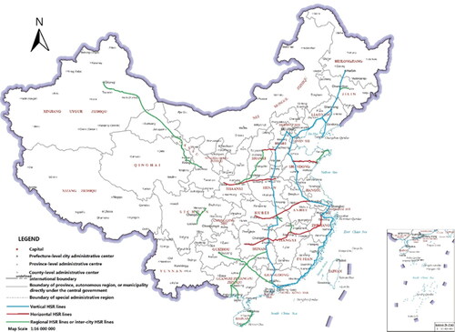
In this paper, we focus on the specific case of the large-scale high-speed rail (HSR) network in China. For China, the HSR network is part of a national strategy to support economic growth and urbanization (Meng et al., 2018). The earlier target of the Chinese HSR network was to form connections between provincial capitals (Ke et al., 2017). Subsequently, China extended the goal of the HSR network to connect medium-sized cities with more than 500,000 people (Shao et al., 2017). Before 2015, 155 out of 292 Chinese cities were connected to the HSR network. At 2016, China’s HSR network running mileage reached 22,000 km, with design speeds ranging from 200 to 350 km per hour (see Figure 1). Growing literature documents a high growth in passenger numbers after HSR services are launched (Vickerman, 2018). In addition, HSR expedites the relocation and band adjustment of corporations and families (Zheng & Kahn, 2013). The likely result is that labor and production resources cluster in cities connected by HSR routes (Shao et al., 2017). Given its substantial impact on the improvement of the accessibility of cities, the HSR system has great potential for nurturing market integration and promoting agglomerated economies and urban growth.

Figure 1. Chinese HSR network before 2015.

Source: Authors.

In this paper, we quantify the economic impact of a large-scale HSR network on cities by comparing the economic performance of a treatment group and a control group before and after the introduction of HSR services. This analysis employs a difference-in-differences (DID) model with a unique dataset: the national train schedules of China between 2007 and 2014. The key identifying assumption is to construct an appropriate counterfactual for what would have happened to cities’ economies in the absence of HSR services. In addition, we employ the instrumental variable (IV) strategy, the PSM-DID methodology and placebo tests to address potential endogeneity concerns. On this basis, we proceed to trace the dynamic effects of the HSR network to investigate whether industrial agglomeration is the mechanism by which HSR promotes the urban economy.

For the eight years before the debut of the HSR services, we find a statistically equivalent trend and level in local GDP for the treatment and control groups. Then, the treatment group experienced significant growth in local GDP after being connected to the HSR network. Our estimates indicate that HSR increases local GDP by approximately 3.3 percentage points on average, which is equivalent to moving a city from the 10th percentile of the city-level GDP distribution to the 29th percentile in 2014. Moreover, our evidence shows a significant increase in industrial agglomeration in the treatment group vis-à-vis the control group after HSR service provision. Moreover, we find that the effect of HSR on regional economic performance is driven partly by the impact of the HSR network on industrial agglomeration.

The remaining parts of this paper proceed as follows. Section 2 reviews the related literature, Section 3 introduces the data and methodology employed in this study, Section 4 presents the results and discusses the econometric analyses, and Section 5 presents the results from the robustness tests. The conclusions and policy implications are addressed in Section 6.

2. Literature review

Our study closely relates to the literature on HSR project cost-benefit analysis (CBA). Whether and to what degree HSR projects affect economic growth are of great importance to policy analysis of new transport infrastructure investments. The coverage of the CBAs of conventional HSR projects naturally varies from country to country, but as a rule, these analyses tend to cover the construction costs of transport projects, the operation and maintenance costs of associated transport services, direct user benefits, and a restricted list of externalities, such as transport safety impacts, congestion, overcrowding and emissions (Ollivier et al., 2014). However, there seems little doubt that there are wider impacts from HSR investment that are not captured by conventional CBA (Laird et al., 2014; Venables, 2007). In particular, the regional economic effect of a large-scale HSR network is considered nontrivial, which should be carefully estimated and added to the extended CBA.

There are intense debates about the causal link between transport and local economic performance (Chen & Vickerman, 2019). The mainstream literature agrees that better transport and better economic performance are causally connected (Vickerman, 2018). Chen (2012) summarizes that this relationship is complex and involve a long-term evolution. Transport infrastructure could produce step changes in accessibility or generalized transport costs. This, in some cases, may lead to significant changes to both individuals and businesses in terms of the location of economic activities (Chen & Vickerman, 2019). From a macroscopic perspective, transport infrastructure could encourage regional economic performance in various aspects, such as enlarging the intercity tourism market, reducing information asymmetry, facilitating innovation and fostering an agglomeration economy (Lawrence et al., 2019).

On the other hand, there is also evidence suggests that this effect is negative or insignificant. Many scholars attaching more value to the safety and efficiency of transportation facilities (Rosová et al., 2013; Sivalai & Rojniruttikul, 2018). Aschauer (1989) states that public investment would crowd out private investment in some scenarios. Huang (2011) concludes that HSR investments crowd out other transportation investments based on the worldwide experience. Besides, Albalate and Fageda (2016) find the provision of HSR services in Spain negatively affected air traffic, which suggests a negative indirect effect of HSR on tourist outcomes. There is also a concern on negative externality of transportation on socioeconomically disadvantaged areas (Faber, 2014). The core-periphery model suggests that transport costs reduction could prompt human and capital in periphery areas to flow towards the core areas and hence weaken the economy development of periphery areas.

New economic geography (NEG) reveals that changes in transport costs and accessibility could, in some cases, have profound effects on the location of agglomeration (Graham, 2007; Krugman, 1991). The extent to which agglomeration occurs depends on the interaction of increasing returns in economic activities, the significance of transport costs and market size (Vickerman, 2008). HSR services contribute to the attractiveness of locations in which industries tend to form spatial clusters based on factors such as increased access to raw materials, technical expertise, and markets. Morten and Oliveira (2016) find that transportation reduces the cost of moving people and promotes interregional migration. International studies suggest that these agglomeration effects are likely to be the most important among the economic effects of HSR (Ollivier et al., 2014).

Chatman and Noland (2011) conduct a detailed literature review on this subject and summarize that transportation improvements can bring substantial positive externalities by enabling economies of agglomeration. Redding and Turner (2015) review the theoretical and empirical literature on how transportation infrastructure modifies the territorial distribution of economic activity. Studies on HSR projects in England, Germany, Spain and Japan also indicate that HSR contributes to an obvious agglomeration effect on regional economies (Hensher et al., 2014; Matas et al., 2020; Wetwitoo & Kato, 2017). Nevertheless, extant empirical works focus mainly on single cities or a narrow spatial domain in which agglomeration effects tend to be obvious (Chen & Vickerman, 2019). The question of whether and to what extent HSR promotes economic performance through the agglomeration effect is still ambiguous, especially for large-scale HSR networks (Shao et al., 2017).

Chen and Vickerman (2017) underline that the agglomeration effect induced by HSR varies in different contexts. In postindustrial places, such as Western Europe, where the secondary industry has largely moved to industrializing countries, the strategic role of HSR is strengthening knowledge economies (Chen, 2012). Evidence also shows that HSR appears to mainly assist in the division of service labor between routine and knowledge-intensive activities in Europe (Chen & Vickerman, 2017). In China, which is still engaged in the industrialization and urbanization process with an extremely uneven pattern (Friedmann, 2005), the situation is different; even though the HSR network has the potential to facilitate agglomeration effects in the industrial and service sectors, the estimation of these effects is inconsistent for cities along different HSR lines. This inconsistency relates fundamentally to the uneven development pattern of secondary industry and the service sector across China. Only some developed cities in the eastern areas of China have experienced the transformation of their service and knowledge-based economies, and most Chinese cities are still important centers of the secondary industry (Chen, 2012; Fang et al., 2020). The related literature on the agglomeration effects of Chinese HSR lines obtains different results in different circumstances. Based on data for 25 cities in China’s Yangtze River Delta region during 1995–2014, Shao et al. (2017) show that HSR has a significant impact on producer service industry agglomeration but not on consumer service industry agglomeration and public service industry agglomeration. Chen and Vickerman (2017) illustrate that in China’s Yangtze River Delta region, some cities with HSR services enjoy strong growth in the secondary industry, while others enjoy strong growth in the service industry. Dai et al. (2018) find that 9 of 14 subdivided industries in the tertiary industry experienced an agglomeration trend in cities with HSR service along the Beijing-Shanghai HSR line after the inauguration of HSR services.

3. Data and methodology

This section describes the data and methodologies employed in this study. Cities in this paper refer to all prefecture-level cities, four province-level cities and fifteen sub-provincial cities in mainland China.

3.1. Data

We collect HSR data from the National Railway Passenger Train Schedule, which contains detailed information on the arrival and departure times of all trains at each station. In 2007, 57 Chinese cities began operating high-speed trains after China’s sixth-round railway large-scale acceleration. Eight cities were connected to the HSR network in 2008, 28 in 2009, 13 in 2010, 1 in 2011, 11 in 2012, 15 in 2013 and 22 in 2014.

The socioeconomic characteristics of cities are collected from the 1999–2014 Statistical Yearbook of Chinese Cities. Datasets on nighttime lights are obtained from the Chinese Research Data Services Platform. The innovation index of cities comes from the China City and Industry Innovation Report (2017). The least-cost HSR route data are from Rao et al. (2019).

Table 1 presents the descriptive statistics¹ with variables measured at the city-year level. Specifically, the data are from 288 cities over a 16-year period from 1999 to 2014. Due to data loss and error, the number of observations in different regressions is different. Based on the GDP deflator of 1978, nominal variables are converted to real variables.

Table 1. Descriptive statistics.

Variable	Obs.	Mean	Std.Dev.
Real GDP/10000 Yuan	1988	14.8	1.156
HSR access	2016	0.375	0.484
Fixed-asset investment/10000 Yuan	1980	14.39	1.095
Total retail sales of consumer goods/10000 Yuan	1985	13.86	1.201
Foreign direct investment/10000 dollar	1785	9.3	1.939
Total population/10000 persons	1990	4.585	0.778
Students enrolled in universities/person	1928	10.38	1.322
Government size/%^a	1983	15.93	8.931
Infrastructure development^b/%	1986	0.012	0.015
Innovation index	2016	7.182	33.61
Density of population/ (people/square kilometers)	2000	6.472	0.953
Secondary industry as Percentage to GDP	2000	51.19	12.19
Tertiary industry as Percentage to GDP	2000	42.04	11.2
Marketization level/%^c	1518	0.475	0.456
The least cost tree	1757	0.315	0.465
Real GDP per capita/Yuan	1971	10.16	0.601
Railway passenger volume/10000 persons	1749	5.788	1.269
Highway passenger volume/10000 persons	1982	8.697	0.976
Average nighttime light brightness	1698	7.122	8.468
Persons employed in manufacturing/person	1977	19.65	1.499
Persons employed in consumer service/person	1973	18.70	1.233
Persons employed in knowledge economy/person	1982	19.06	1.090

Note: The cross-city standard deviation of $Y$ is the standard deviation of ($Y_{st}-\widetilde{Y_s}$), where $\widetilde{Y_s}$ is the average value of Y in city s over the sample period.

^a Government size is measured by the ratio of government expenditure to GDP.

^b Infrastructure development refers to the value area of paved roads divided by total land area of city.

^c Marketization level is expressed by the proportion of foreign investment to GDP.

Source: Authors.

3.2. Methodology

We use the DID method to identify the economic impact of the HSR network and further resolve the endogenous HSR route placement concern with multiple strategies (the IV strategy, PSM-DID, and placebo tests). Drawing on the work of Beck et al. (2010), a continuous DID model is used and presented as follows: (1) $$Y_{s,t}=\alpha +\beta HS{R}_{s,t}+\mathit{\delta }{X}_{s,t}+{\mathit{A}}_{\mathit{s}}+{\mathit{B}}_{\mathit{t}}+{ϵ}_{s,t}\mathrm{}$$(1)

In Equation (1), $Y_{s,t}$ is a measure of the economic development of city s in year t. A_s and B_t are vectors of city and year dummy variables that account for city and year fixed effects, respectively; X_st is a set of time-varying, city-level control variables, and ε_st is the error term. The variable of interest is $HS{R}_{s,t},$ a dummy variable that equals one in the years after city s initiates HSR service and equals zero otherwise. The coefficient β reflects the impact of the HSR network on urban economic performance. Year-specific dummy variables control for nationwide shocks and trends that shape economic development over time, such as business cycles, policy changes, and changes in labor force participation. City-specific dummy variables control for time-invariant, unobserved city characteristics that affect economic development across cities.

Following Beck et al. (2010), we use the following regression to test for a common pretreatment trend for the control group and treatment group: (2) $$Y_{s,t}=\alpha +{\beta }_1{D}_{s,t}^{-10}+{\beta }_2{D}_{s,t}^{-9}+\dots {+\beta }_{17}{D}_{s,t}^6+{\beta }_{18}{D}_{s,t}^7+{\mathit{A}}_{\mathit{s}}+{\mathit{B}}_{\mathit{t}}+{ϵ}_{s,t}\mathrm{}$$(2)

In Equation (2), we incorporate a set of indicator variables (the ‘Ds’) corresponding to 1 year, 2 years,$\mathrm{}\cdots ,$ before or after HSR services were introduced. Specifically, for the notation of $D_{s,t}^{\pm j},$ the ‘$j$’ is a superscript of these indicator variables, and we put a minus or plus sign before the ‘$j$’ to denote the $j$ year before or after the year city $s$ connected to the HSR network. $D_{s,t}^{-j}\mathrm{}({or\mathrm{}D}_{s,t}^{+j})\mathrm{}$ measures whether year $t$ is the $j$ year before (or after) city $s$ is connected to the HSR network. $D_{s,t}^{-j}$ equals one for city $s$ in the $j$ year before it is connected to the HSR network and equals zero otherwise. $D_{s,t}^{+j}$ equals one for city $s$ in year $j$ after it is connected to the HSR network and equals zero otherwise. ${\mathit{A}}_{\mathit{s}}\mathrm{}$ and ${\mathit{B}}_{\mathit{t}}$ are vectors of city and year dummy variables that account for city and year fixed effects, respectively.

Following the literature (Faber, 2014; Rao et al., 2019), we adopt the least-cost path HSR network computed by Rao et al. (2019) as the IV. The least-cost tree network refers to the hypothetical HSR routes with the lowest construction cost between major cities, which are constructed considering geographic characteristics (slope, relief degree of the land surface, etc.). The combination of propensity score matching (PSM) and the double-difference method is used to mitigate the endogeneity caused by selective biases from observable variables. Moreover, we conduct a placebo test by randomly assigning the choices of HSR services to cities to examine whether the results are influenced by omitted variables (Chetty et al., 2009; Li et al., 2016).

4. Results and discussion

4.1. Preliminary tests

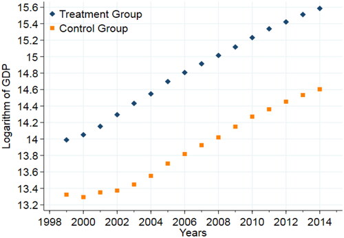
The State Council noted in its 2008 edition of the Mid-to-Long Term Railway Development Plan that the goal of HSR is to connect provincial capital cities and central cities. This goal explains the phenomenon observed in China well—cities with large populations and a large economy or political importance are the first to be included in the HSR network. It can be concluded from Figure 2 that during the 1999–2014 period, the economic strength of cities served by the HSR network is stronger than that of cities without HSR services.

Figure 2. The trend of the average local GDP of cities.

Source: Authors.

Considering that the ‘winner’ cities are those that do or are expected to perform well, it is difficult to disentangle the effects of HSR from the natural growth path. Urban economic performance and HSR connection are correlated; hence, estimations that do not tackle this endogenous route placement are likely to be biased. In this article, our solution is establishing an appropriate counterfactual for ‘winner’ cities. The large-scale HSR network facilitates the identification of suitable counterfactuals. We first look at Figure 3—the histograms of the average local GDP (1999–2006) of ‘winner’ cities and ‘loser’ cities.²

Figure 3. Histograms of average local GDP (1999–2006).

Source: Authors.

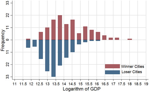
As shown in Figure 3, in terms of economic performance, some of the ‘winner’ cities far exceed other cities, and some of the ‘loser’ cities lag far behind other cities. For both groups, it is difficult to find a suitable counterfactual for what would have happened in the absence or presence of HSR services. However, for other ‘winner’ cities, it seems possible to construct feasible counterfactuals because Figure 3 shows that many of the ‘winner’ cities and ‘loser’ cities have similar economic volumes, as measured by the average level of GDP in 1999–2006.

We construct the counterfactual for ‘winner’ cities by matching each of them with a loser city featuring a close average GDP level and GDP growth trend in 1999–2006. The specific procedure is as follows:

1. we calculate the average GDP of all cities during 1999–2006.

2. search for potential counterfactuals for each winner city based on average GDP. A loser city is defined as a potential counterfactual for a winner city if the difference on average GDP between them was below 300 million RMB yuan, less than 10% of the average GDP of all cities before 2007.

3. draw the GDP trends for each winner city and its potential counterfactuals, and then select one city which has a GDP trend similar to that of the winner city as its counterfactual.

The matched sample includes 64 ‘winner’ cities (the treatment group) and 64 ‘loser’ cities (the control group).³ This matching method stresses the similarity of economic development between the treatment group and the control group. There are also some limitations of this matching method. First, the poorest and richest cities are discarded from the sample because there is no appropriate counterfactual for them. The estimation bias might arise because discarded samples are systematically different from those retained. Second, our procedure shares the same limitation as the Synthetic Control Approach, namely that there still remains uncertainty about the power of the control group to reproduce the counterfactual outcome trajectory that the treatment group would have experienced in the absence of treatment. In this paper, we employ a set of robust tests (full-sample regression, IV strategy, placebo tests, etc.) to alleviate these concerns.

We believe that the control group forms a reliable counterfactual for the treatment group. First, Figure 4 indicates that before 2007, the level and trend of GDP of these two groups were very similar. Second, Figure 5 shows that there is no evident trend in the difference between the control group and treatment group in terms of the average logarithm of GDP. It is well recognized that many confounding factors, which are observable or not, affect economic development, but the aggregate effects of those determinants did not significantly distinguish the control group from the treatment group. If there are no systemic shocks for the control group or treatment group, the similarity of their economic performance and trend will continue to exist.

Figure 4. The logarithm of GDP for the treatment group and control group.

Source: Authors.

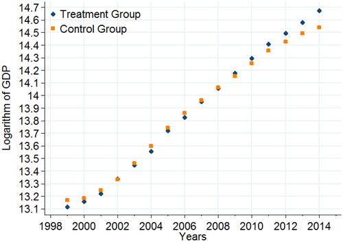
Figure 5. The difference in GDP between the control group and treatment group.

Source: Authors.

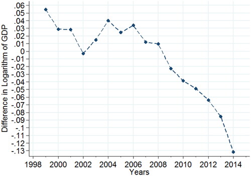
Moreover, the economic performance of the control group was even slightly stronger than that of the treatment group before 2007. Notably, after 2007, the year HSR services were launched in China, the difference between the control group and treatment group in the average logarithm of GDP shows a downward trend until 2014. That is, the economic strength of the treatment group caught up and surpassed that of the control group after the introduction of HSR services.

4.2. DID analyses

We employ the DID specification—equation (1)—to assess the economic effect of the HSR network in Table 2. All models control for city and year fixed effects. The first and third models in Table 2 do not include control variables,⁴ but the second and fourth models do.

Table 2. DID regressions.

Ln(GDP)	Full-Sample		Matched sample
	Model (1)	Model (2)	Model (3)	Model (4)
HSR	0.021	0.023*	0.114***	0.033***
	(0.027)	(0.013)	(0.040)	(0.015)
Control	No	Yes	No	Yes
Cons	14.379***	5.996***	13.936***	5.910***
	(0.010)	(0.735)	(0.0129)	(0.807)
Year Fixed Effect	Yes	Yes	Yes	Yes
City Fixed Effect	Yes	Yes	Yes	Yes
Observations	2271	1654	1017	767
R-square	0.779	0.924	0.768	0.930

Note: Standard errors are adjusted for city level clustering and appear in parentheses. *, **, and *** indicate statistical significance levels at the 10%, 5%, and 1% levels, respectively. Covariates variables include fixed-asset investment, total retail sales of consumer goods, foreign direct investment, total population, students enrolled in universities, government size, infrastructure development, innovation index, density of population, secondary industry as percentage to GDP, tertiary industry as percentage to GDP, marketization level. Same hereinafter.

Source: Authors.

The first two columns using the full-sample regression indicate that the HSR network leads to an increase in local GDP of 2% or so. In the first column, the coefficient of the effect of the provision of HSR services has no statistical significance. This could be attributed to the omission of the impacts of time-varying urban properties. However, after the incorporation of these time-varying controls, in the second column, the R-square of this regression increases substantially to 0.924, and the coefficient reaches the 10% level, which is statistically significant. Similarly, the variation between the coefficients in columns (3) and (4) shows that these time-varying controls matter for urban economic development.

As discussed in the above subsection, the control group for the matched sample is an appropriate counterfactual to the treatment group. Thus, we use the matched sample in columns (3) and (4). The estimates of the HSR effect in columns (3) and (4) satisfy significance criteria at the 1% level, and both are larger than the estimates yielded by the full-sample regression. These differences highlight that the close economic strength and growth trend that existed prior to the introduction of HSR services affects the estimation of the impact of the HSR network. It is reasonable to speculate that the full-sample regressions may underestimate the economic effect of the HSR network.

Model 4 suggests that the average treatment effect of the HSR network on local GDP is 0.033, which amounts to 0.7 billion RMB yuan per year. The effect of the HSR network on local GDP is equivalent to moving a city from the 10th percentile of the city-level GDP distribution to the 29th percentile. Overall, Table 2 relatively consistently points to a positive and significant impact of HSR on local GDP. These results are consistent with previous literature on the economic effects of HSR. Meng et al. (2018) find that the ATT of HSR construction on county-level economic growth is approximately 14%. Ahlfeldt and Feddersen (2018) find a causal effect of HSR introduction on the average GDP of three counties with intermediate stops, more specifically, an increase of approximately 8.5%. The baseline estimate is consistent with the circumstantial evidence presented in Figures 4 and 5 and is robust to a series of tests.

4.3. Dynamics of the economic effects of the HSR network

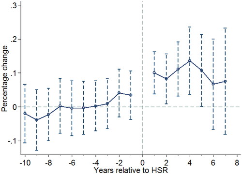
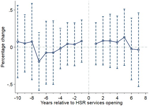
The figure plots the impact of the HSR network on the natural logarithm of GDP. We consider a 17-year window spanning from ten years before the launch of the HSR network until seven years after the launch. The dashed lines represent 95% confidence intervals, adjusted for city-level clustering. There is much greater variance in the estimates of the economic effects six or seven years after HSR opening; hence, the estimates may be measured with less precision. Specifically, we report the estimated coefficients in equation (2), accounting for city and year fixed effects. Following Beck et al. (2010), we exclude the year the HSR network was launched to estimate the dynamic effects of HSR on local GDP relative to the launch year.

Figure 6 illustrates two key points. First, changes in the difference in local GDP between the treatment group and control group did not precede the launch of the HSR network. As shown, the coefficients on the pre-HSR dummy variables are insignificantly different from zero for all years before the HSR launch, with no trend in local GDP prior to the launch. This establishes the parallel trend assumption between the treatment group and control group, which provides a solid basis for the DID analyses. Second, the positive impact of HSR on local GDP emerges after the provision of HSR services and remains significant at the 5% level until five years after the launch of the HSR network. In sum, changes in local GDP do not precede the provision of HSR services, and HSR service has a promotion effect on local GDP.

Figure 6. Dynamics of the economic effects of the HSR network.

Source: Authors.

4.4. Channels of the economic impact of the HSR network

In this subsection, we explore whether HSR service provision gives rise to industrial agglomeration or service agglomeration, which is the potential channel underlying the economic impact of the HSR network.

4.4.1. Industrial agglomeration effect

We first investigate whether the HSR network induces industrial enterprises to cluster towards the treatment group by using equation (2) with a 17-year window to track annual changes in several indicators of industrial agglomeration before and after the launch of the HSR network.

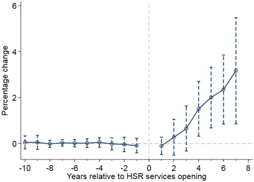
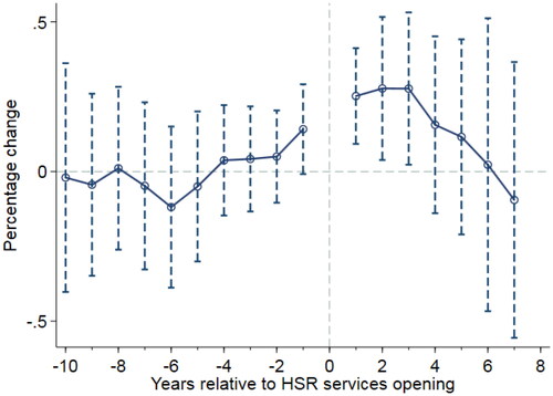
Figures 7–10 plot the annual impact of the HSR network on the number of industrial enterprises, gross industrial output, persons employed in manufacturing and the ratio of gross industrial output to local GDP (gross industrial output value/GDP). The dashed lines represent 95% confidence intervals, adjusted for city-level clustering. Following Beck et al. (2010), we exclude the year of HSR opening, thus estimating the dynamic effects of HSR relative to the year of HSR opening.

Figure 7. Logarithm of the number of industrial enterprises.

Source: Authors.

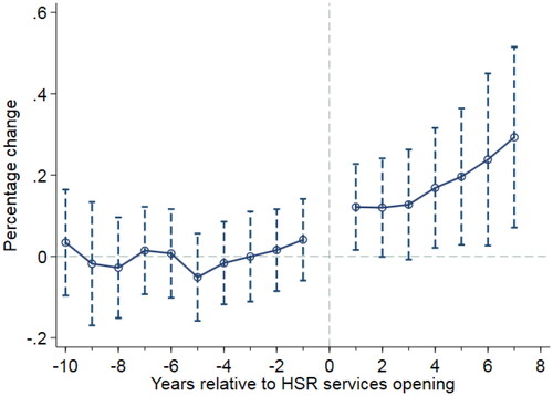
Figure 8. Logarithm of gross industrial output.

Source: Authors.

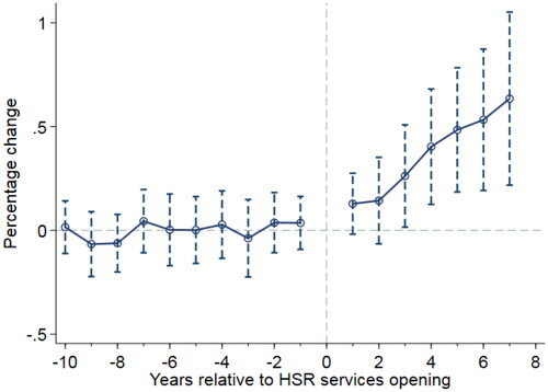
Figure 9. Logarithm of the number of people employed in manufacturing.

Source: Authors.

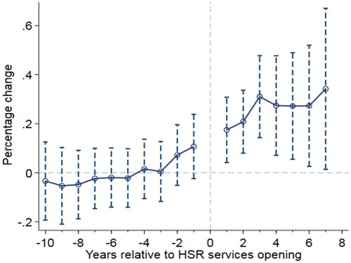
Figure 10. The ratio of industrial output to local GDP.

Source: Authors.

Figure 7 indicates that more industrial enterprises cluster to the treatment group than to the control group after the launch of the HSR network. The difference in the number of industrial enterprises is insignificant for all years before HSR launch. While the number of industrial enterprises in the treatment group shows a significant increase after the launch of the HSR network, an upward trend continues thereafter, with an overall increase of almost 30% seven years after the launch.

Figure 8 shows that the HSR network leads to a significant increase in the gross industrial output of the treatment group vis-à-vis the control group. An upward trend starts two years after the launch of the HSR network and continues for the following five years, with an overall increase of almost 30%.

Figure 9 shows the number of people employed in manufacturing in the treatment group vis-à-vis the control group increase immediately after HSR network launch, and the effects remain positive and significant at the 5% level. The impacts grow for approximately two years after HSR opening and then level off, indicating a steady increase in the number of people employed in manufacturing of approximately 30%.

Having found that the HSR network induces the spatial concentration of industry enterprises and boosts gross industrial output, we now explore whether industrial agglomeration enhancement stimulates urban economic performance. Specifically, we first calculate the ratio of industrial output to GDP. Then, we trace the annual changes in the ratio between the treatment group and the control group.

Figure 10 shows an upward trend in the ratio of industrial output to GDP starting immediately after the launch of the HSR network and lasting for the following six years. The effects of HSR service provision become significant at the 5% level beginning in the fourth year after HSR network launch, with an overall increase of approximately 40%.

This subsection reveals a significant increase in industrial agglomeration in the treatment group vis-à-vis the control group after the introduction of HSR services, and industrial agglomeration further gives rise to disparities in regional economic performance. Our results are consistent with extant studies on the relationship between transportation and industrial agglomeration (Wetwitoo & Kato, 2017).

4.4.2. Service agglomeration effect

We now investigate whether the HSR network induces service agglomeration by using equation (2) with a 17-year window to track annual changes in several indicators of service agglomeration before and after the launch of the HSR network.

Figures 11–15 plots the annual impact of the HSR network on the number of persons employed in the service sector, finance, ICS (information transmission, computer services and software), WR (wholesale and retail trade), and hotels and catering services. The dashed lines represent 95% confidence intervals, adjusted for city-level clustering. Following Beck et al. (2010), we exclude the year the HSR network was launched, thus estimating the dynamic effects of HSR relative to the year of launch.

Figure 11. Logarithm of the number of people employed in the service sector.

Source: Authors.

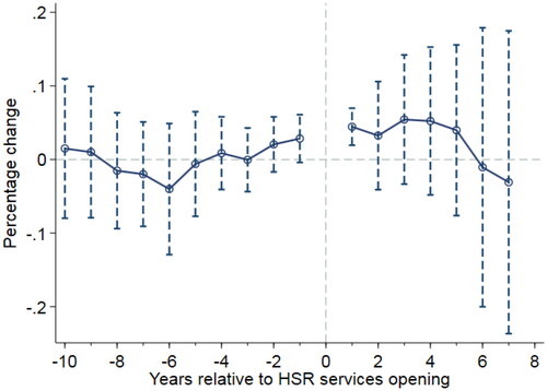
Figure 12. Logarithm of the number of people employed in finance.

Source: Authors.

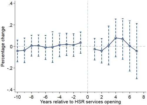
Figure 13. Logarithm of the number of people employed in information transmission, computer services and software.

Source: Authors.

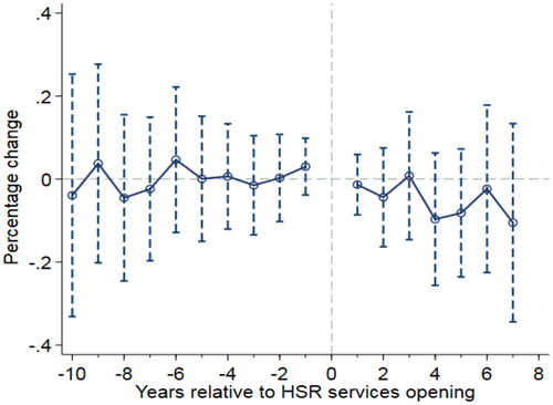
Figure 14. Logarithm of the number of people employed in wholesale and retail trade.

Source: Authors.

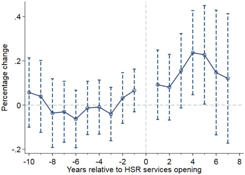
Figure 15. Logarithm of the number of people employed in hotels and catering services.

Source: Authors.

Figures 11–15 seemingly indicate that the introduction of HSR services has no significant and consistent impact on service agglomeration. There are some short-term shocks in some service industries (Figures 11, 14 and 15) after the launch of HSR services, but these effects quickly fade, and the differences between the treatment group and control group become insignificant. In addition, Figures 12 and 13 show no differences in the scale of financing and ICS between the treatment group and control group before and after the introduction of HSR services. Thus, we cannot reject or accept the potential effect of HSR services without any solid evidence.

It may be that HSR does not change the absolute size of the service sector or certain service industries but could lead to a significant transformation in service sectoral specialization patterns. In particular, it would be interesting to determine whether there are any changes in the relationship between cities with and without HSR services in terms of specialization. To do this, we construct the two indexes to measure the diversification and specialization of the service sector. The first is the index of service sector specialization, $\mathit{ISS},$ which is usually defined as (3) $$\mathit{ISS}=\max (P_{\mathit{ijt}}/P_{jt})\mathrm{}$$(3) where $P_{\mathit{ijt}}$ is the share of employment in industry $j$ in the total employment in the service sector in city $i$ in year $t.$ $P_{jt}$ is the share of employment in industry $j$ in the total employment in the service sector of all cities in year $t.$ $P_{jt}$ is the service sector employment structure benchmark. If $\mathrm{I}SS$ is greater than 1, the degree of specialization in the service sector in city $i$ is higher than the benchmark. The higher $\mathit{ISS}$ is, the higher the level of specialization in the service sector in city $i.$

The second is the index of service sector diversification, $\mathit{ISD},$ which is defined as (4) $$\mathit{ISD}=\frac{1}{{\sum }_j\left|P_{\mathit{ijt}}-P_{jt}\right|}\mathrm{}$$(4)

Essentially, this index is a way to characterize how the employment structure of a city is different from the benchmark. It can be easily verified that the more diverse a city's service sector is, the smaller the denominator of equation (3)(5) $$p\left({\mathbf{X}}_{\mathrm{s}}\right)=Pr({\mathrm{Treatment}}_{\mathrm{s}}=1|{\mathit{X}}_s)=\mathit{F}(h\left({\mathit{X}}_s\right))$$(5) is, and thus, the larger the $\mathit{ISD}$ is.

Figures 16–17 plots the annual impacts of the HSR network on the diversification and specialization of the service sector. These two graphs show that there are no significant changes in the service sector specialization and diversification level between the treatment group and control group after HSR network launch.

Figure 16. The index of service sector specialization.

Source: Authors.

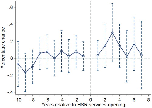
Figure 17. The index of service sector diversification.

Source: Authors.

Even though HSR has the potential to facilitate industrial and service agglomeration, our empirical results only verify the industrial agglomeration effect. This may relate to the uneven development of the service sector between different regions. In China, only some economically prosperous cities in the eastern district have experienced the transformation of their service and knowledge-intensive economy, and most secondary cities are still dominant in the secondary industry. In this context, large cities with large-scale service sectors in the eastern region might enjoy possible service agglomeration induced by the HSR network. This assumption is supported by existing studies (Dai et al., 2018; Shao et al., 2017). The matched sample does not include economically prosperous cities. Thus, it is not surprising that we do not find a significant service agglomeration effect. However, this does not mean that there is no service agglomeration effect, which might exist in some metropolitan areas along some HSR lines in the eastern region of China. In general, we only find the industrial agglomeration effect induced by the HSR network in China.

5. Robustness tests

In this section, robustness tests, including the IV strategy, PSM-DID methodology, placebo tests and sensitivity tests, are used to address various concerns.

5.1. IV Strategy

To address nonrandom HSR route placements between cities, we use an instrumental variable strategy based on the construction of the least-cost path spanning tree network. This concept comes from Faber (2014) and has been advanced by a great body of literature. Rao et al. (2019) develop it for the least-cost HSR network—the hypothetical HSR routes with the lowest construction cost between major cities. They compute the least-cost path network between all major city pairs on the basis of geographical features (land cover and elevation). This strategy identifies the subset of routes that connect target cities on a single continuous network subject to construction cost minimization. Obviously, the hypothetical HSR routes are highly correlated with cities’ geographical characteristics but not their recent economic development. Our IV is the least-cost HSR network constructed by Rao et al. (2019).

Following Diao (2018), we first estimate a probit regression with the IV and a set of city-level characteristics (population, GDP per capita, and train passengers) to predict the likelihood that a city will receive HSR service after 2006. Then, the predicted probability is integrated into the second stage of the DID specification.

column (2) of Table 3 presents the first-stage probit estimates. The dependent variable in this regression is a dummy variable HSR_i, which equals one if city i obtained an HSR connection after 2006 and zero otherwise. The IV is PHR_i (short for potential HSR routes), a dummy variable that equals one if city s is located in the least-cost HSR network and zero otherwise. The results show that the likelihood of receiving HSR service is positively related to the IV, which suggests that the least-cost HSR network is a good predictor of receiving HSR service, conditional on control variables.

Table 3. IV Regression.

First-stage probit regression		Second-stage regression
HSR	Model (5)	Ln(GDP)	Model (6)
Potential HSR Route	0.847***	HSR	0.126***
	(0.125)		(0.053)
Population	0.440***
	(0.105)
GDP Per Capita	0.442***
	(0.110)
Train Passengers	0.975***
	0.076	Control	Yes
Constant	Yes	Constant	Yes
LR Chi2	334.95	Year Fixed Effect	Yes
Year Fixed Effect	Yes	City Fixed Effect	Yes
Pseudo R2	0.205	R-square	0.920
Observations	1691	Observations	1880

Source: Authors.

column (4) of Table 3 reports the second-stage results of the IV regression. Consistent with Subsection 4.2, the coefficients for the HSR connection are significantly positive, indicating that the baseline DID estimate of the economic effect of the HSR network is robust to potential endogeneity concerns.

5.2. Psm-DID analyses

In this subsection, we use the combination of propensity score matching (PSM) and DID to mitigate potential endogeneity-related selective biases caused by observable variables. The first step is to estimate the conditional probability (propensity score) that a city will receive HSR service. We use pre-HSR setup data to run the probit model.

The probit specification is presented as follows: (5) $$p\left({\mathbf{X}}_{\mathrm{s}}\right)=Pr({\mathrm{Treatment}}_{\mathrm{s}}=1|{\mathit{X}}_s)=\mathit{F}(h\left({\mathit{X}}_s\right))$$(5)

$p({\mathit{X}}_s)$ is defined as the probability of city s receiving the treatment—HSR service—conditional on a set of observed covariates ${\mathit{X}}_s.$ $\mathit{Treatment}$_s is a dummy variable that equals one if city s was connected to the HSR network during 2007–2014 and zero otherwise. $\mathit{F}$ is the probability function of the linear combination of covariates ${\mathit{X}}_{\mathit{s}}—h\left({\mathit{X}}_s\right).$ X_s is a vector of covariates including total population, GDP per capita, the relief degree of the land surface, railway and highway passenger volume. These indicators reveal the political importance, economic prosperity, HSR service demand and feasibility of a city. These control variables are set as the arithmetic mean of 8 years (1999–2006).

The second step is to construct the treatment group and control group for DID analyses by matching ‘winner’ cities with ‘loser’ cities one by one based on propensity scores. The score caliper of one-to-one matching is set as 0.03. Then, the DID specification is used to test for the economic effects of the HSR network.

Table 4 shows that the HSR dummy enters positively and significantly in all PSM-DID regressions. The results substantiate the positive effect of the HSR network and confirm the reliability of the baseline estimation.

Table 4. PSM-DID Regressions.

Ln(GDP)	Model (7)	Model (8)
HSR	0.064***	0.039***
	(0.033)	(0.013)
Controls	No	Yes
Cons	14.204***	6.403***
	(0.011)	(0.802)
Year Fixed Effect	Yes	Yes
City Fixed Effect	Yes	Yes
Observations	1324	1069
R-square	0.795	0.926

Source: Authors.

5.3. Placebo tests

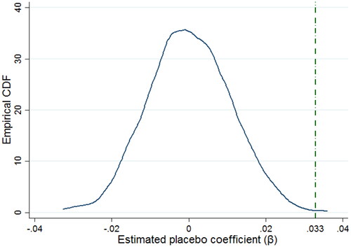
In this subsection, placebo tests are employed to examine whether the results are influenced by potential omitted variables. Following previous studies (Chetty et al., 2009; Li et al., 2016), the first step is to randomly allocate the HSR service provision timing of ‘winner’ cities. Then, DID estimation is performed with virtual ‘winner’ cities and ‘loser’ cities. This procedure was repeated 1,000 times to increase the identification power of these falsification tests. Given the random data generation process, the ‘virtual’ HSR connection variables should produce no significant estimates with a magnitude close to zero.

Figure 18 shows the distribution of the estimates from the 1,000 runs along with the benchmark estimate, 0.033, from column 4 in Table 2. The CDF of estimates from random HSR connection assignments is clearly centered around zero, and the standard deviation of the estimates is 0.011, suggesting that there is no effect with the random HSR connection assignment. The benchmark estimate is located outside the 99% confidence interval of the distribution (1 out of 1000 estimates larger than 0.033). The placebo tests suggest that the positive and significant effect of the HSR connection on economic performance is not driven by unobserved factors.

Figure 18. Placebo tests.

Source: Authors.

5.4. Sensitivity tests

We perform sensitivity tests with the following strategies. First, we expand the sample from 128 to 170 cities by relaxing the matching criteria⁵ carried out in Subsection 4.1. Second, we expand the sample period from 2007–2014 to 1999–2014.

Third, we substitute the dependent variable from local GDP to the average brightness of lights at nighttime. Nighttime lightness data are gradually perceived as an effective measurement index related to urban economic development since Henderson et al. (2012) demonstrate that nighttime light data can serve as a substitute proxy for GDP over the long term and track short-term fluctuations in growth.

We emphasize that there are several open questions regarding the use of light data as a proxy for local economic development. First, there might be some areas for which light data have insufficient resolution, which causes high measurement error. Second, some nighttime light data may not be suitable for GDP estimation at the city level because the analysis unit is small and the light overflow and saturation phenomenon are significant (Dai et al., 2017). In addition, the accuracy of GDP estimation based on nighttime light data is affected by the spatial scale of the study area, the density, the land cover types and the industrial structures of the study area. On the other hand, the use of nighttime light data in sensitivity tests has two advantages. One is that the nighttime lightness intensity is strongly associated with economic performance and development, and the other is that it is free from human errors and manipulation (Henderson et al., 2012). Overall, we consider that light data may be a useful supplemental variable to local GDP.

As shown in Table 5, the HSR dummy variables are positive and significant on at least the 10% level in all regressions, which indicates that the baseline results are robust to sensitivity tests.

Table 5. Sensitivity tests.

	170 samples		1999–2014		Nighttime light data
	Ln(GDP)	Ln(GDP)	Ln(GDP)	Ln(GDP)	Dnvalue	Dnvalue
HSR	0.093***	0.040***	0.089**	0.043**	0.166**	0.159*
	(0.033)	(0.013)	(0.037)	(0.018)	(0.080)	()0.088
Control	No	Yes	No	Yes	No	Yes
Cons	14.163***	6.024***	13.151***	6.168***	4.504***	1.542
	(0.011)	(0.734)	(0.021)	(0.959)	(0.033)	(3.971)
Year Fixed Effect	Yes	Yes	Yes	Yes	Yes	Yes
City Fixed Effect	Yes	Yes	Yes	Yes	Yes	Yes
Observations	1353	1077	1903	1336	756	666
R-square	0.775	0.926	0.882	0.947	0.551	0.572

Source: Authors.

6. Conclusions

This paper tries to test for and quantify the effect of the HSR network on urban economic development. Moreover, we further investigate whether industrial or service agglomeration is the mechanism by which the HSR network promotes urban economic performance. Our analyses are based on the rapid development of the HSR network in China. This large-scale HSR network enables us to construct an appropriate counterfactual for what would have happened to cities’ economies in the absence of HSR services, which is the key prerequisite for causality identification.

In this study, we employ national train schedules during the 2007–2014 period and apply DID and other empirical strategies to evaluate the average treatment effect of the HSR network on local GDP. After controlling for time-varying variables and time-invariant city characteristics, HSR network connection contributes to a 3.3-percentage-point relative increase in local GDP. Numerous robustness tests confirm our baseline estimation. Our estimation also suggests that the uneven development gap between the ‘winner’ cities and ‘loser’ cities in China will increase because of the development of the HSR network.

Regarding the mechanism through which the HSR network boosts the local economy, dynamic analyses suggest that HSR service provision gives rise to industrial agglomeration, which then promotes local GDP, at least in part. However, the fact that industrial agglomeration does not fully account for the whole economic effect of the HSR network underscores that there remains much to learn about the structural source of estimated spillovers from the HSR network. Moreover, we do not find any valid evidence of the service agglomeration effect using the matched sample. This result may be related to the specific economic trajectory of China. In contrast to cities in developed countries that have shifted from the industrial economy to the knowledge economy, most Chinese cities are still becoming industrialized and urbanized. Therefore, only some major cities with a large-scale service sector are likely to benefit from the service agglomeration effect induced by HSR. It is worth noting that the economic contexts in parallel with HSR development should not be ignored.

Our results will help quantitatively measure the economic impact of the HSR network that is not, or not fully, accounted for by conventional transport CBA. Thus, our findings have important policy implications for countries that plan to upgrade their railway systems to accommodate increasing interregional transportation demand and stimulate regional economic development. In addition, our results are also meaningful for the layout of HSR routes in light of their positive impacts on the economic distribution landscape. For instance, to drive the development of inland areas, the Chinese HSR network gradually expands to the central and western regions, which are not economically developed places.

We acknowledge that this article still has insufficiencies and limitations. For instance, we now cannot differentiate between the direct, indirect, and induced effects of the HSR network. With comprehensive and feasible studies in the future, there might be some interesting and important findings in this field. Second, given the importance of tourism for local GDP, the effects of the HSR network on tourism need to be explored with detailed data.

Disclosure statement

No potential conflict of interest was reported by the author(s).

Additional information

Funding

This study is funded by the National Social Science Foundation of China (Grant No. 20BJY049).

Notes

1 The city here refers to the municipal district, not the entire city including municipal districts, counties and county-level cities. In addition, all variables in table 1, except for Dnvalue, Logtrainps, Logroadps and Logfre, refer to data on municipal districts.

2 The ‘winner’ cities refer to cities that were connected to the HSR before 2014, and the ‘loser’ cities refer to cities that had no HSR access before 2014.

3 Due to space limitations, more specific information about the matched sample can be obtained by e-mail to the authors.

4 The control variables of the model include fixed asset investment, total retail sales of social consumer goods, foreign direct investment, total population at the end of the year, students enrolled in universities, government size, infrastructure development, the innovation index, secondary industry as a percentage of GDP, tertiary industry as a percentage of GDP, the marketization level, and population density.

5 The difference between each winner city and its candidate counterfactuals are set to below 300 million yuan, less than 10% of the average GDP of all cities before 2007. Then, we expand the sample to 170 cities by loosening the difference to 50% of the average local GDP of all cities before 2007.

References

- Ahlfeldt, G. M., & Feddersen, A. (2018). From periphery to core: Measuring agglomeration effects using high-speed rail. Journal of Economic Geography, 18(2), 355–390. https://doi.org/10.1093/jeg/lbx005
- Albalate, D., & Fageda, X. (2016). High speed rail and tourism: Empirical evidence from Spain. Transportation Research Part A: Policy and Practice, 85, 174–185.
- Aschauer, D. (1989). Is public expenditure productive? Journal of Monetary Economics, 23(2), 177–200. https://doi.org/10.1016/0304-3932(89)90047-0
- Banerjee, A., Duflo, E., & Qian, N. (2020). On the road: Access to transportation infrastructure and economic growth in China. Journal of Development Economics, 145, 102442. https://doi.org/10.1016/j.jdeveco.2020.102442
- Beck, T., Levine, R., & Levkov, A. (2010). Big bad banks? The winner and loser from bank deregulation in the United States. The Journal of Finance, 65(5), 1637–1667. https://doi.org/10.1111/j.1540-6261.2010.01589.x
- Chatman, D. G., & Noland, R. B. (2011). Do public transport improvements increase agglomeration economies? A review of literature and an agenda for research. Transport Reviews, 31(6), 725–742. https://doi.org/10.1080/01441647.2011.587908
- Chen, C. (2012). Reshaping Chinese space-economy through high-speed trains: Opportunities and challenges. Journal of Transport Geography, 22, 312–316. https://doi.org/10.1016/j.jtrangeo.2012.01.028
- Chen, C., & Vickerman, R., (2019). Quantifying the economic and social impacts of High-Speed rail: Europe and the People's Republic of China. In Y. Hayashi, K. S. Ram, & S. Bharule (Eds.), Handbook on high-speed rail and quality of life (pp. 283–303). ADB. Retrieved from https://papers.ssrn.com/sol3/papers.cfm?abstract_id=3637158
- Chen, C., & Vickerman, R. (2017). Can transport infrastructure change regions' economic fortunes? Some evidence from Europe and China. Regional Studies, 51(1), 144–160. https://doi.org/10.1080/00343404.2016.1262017
- Chetty, R., Looney, A., & Kroft, K. (2009). Salience and taxation: Theory and evidence. American Economic Review, 99(4), 1145–1177. https://doi.org/10.1257/aer.99.4.1145
- Dai, Z., Hu, Y., & Zhao, G. (2017). The suitability of different nighttime light data for GDP estimation at different spatial scales and regional levels. Sustainability, 9(2), 305. https://doi.org/10.3390/su9020305
- Dai, X., Xu, M., & Wang, N. (2018). The industrial impact of the Beijing-Shanghai high-speed rail. Travel Behaviour and Society, 12, 23–29. https://doi.org/10.1016/j.tbs.2018.03.002
- Diao, M. (2018). Does growth follow the rail? The potential impact of high-speed rail on the economic geography of China. Transportation Research Part A: Policy and Practice, 113, 279–290. https://doi.org/10.1016/j.tra.2018.04.024
- Faber, B. (2014). Trade integration, market size, and industrialization: Evidence from China's national trunk highway system. The Review of Economic Studies, 3, 1046–1070.
- Fang, L., Zhang, X., Feng, Z., & Cao, C. (2020). Effects of high-speed rail construction on the evolution of industrial agglomeration: Evidence from three Great Bay Areas in China. E + M Ekonomie a Management, 23(2), 17–32. https://doi.org/10.15240/tul/001/2020-2-002
- Friedmann, J. (2005). China's urban transition. University of Minnesota Press.
- Graham, D. J. (2007). Variable returns to agglomeration and the effect of road traffic congestion. Journal of Urban Economics, 62(1), 103–120. https://doi.org/10.1016/j.jue.2006.10.001
- Henderson, J. V., Storeygard, A., & Weil, D. N. (2012). Measuring economic growth from outer space. American Economic Review, 102(2), 994–1028. https://doi.org/10.1257/aer.102.2.994
- Hensher, D. A., Ellison, R. B., & Mulley, C. (2014). Assessing the employment agglomeration and social accessibility impacts of high-speed rail in Eastern Australia. Transportation, 41(3), 463–493. https://doi.org/10.1007/s11116-013-9480-7
- Huang, T. (2011). Financial impacts of and financing methods for high-speed rail in Portugal [Doctoral dissertation]. Massachusetts Institute of Technology.
- Ke, X., Chen, H., Hong, Y., & Hsiao, C. (2017). Do China's high-speed-rail projects promote local economy? —New evidence from a panel data approach. China Economic Review, 44, 203–226. https://doi.org/10.1016/j.chieco.2017.02.008
- Krugman, P. (1991). Increasing returns and economic geography. Journal of Political Economy, 99(3), 483–499. https://doi.org/10.1086/261763
- Laird, J., Nash, C., & Mackie, P. (2014). Transformational transport infrastructure: Cost-benefit analysis challenges. Town planning review, 85(6), 709–730. https://doi.org/10.3828/tpr.2014.43
- Lawrence, M., Bullock, R., & Liu, Z. (2019). China's high-speed rail development. World Bank Publications.
- Li, P., Lu, Y., & Wang, J. (2016). Does flattening government improve economic performance? Evidence from China. Journal of Development Economics, 123, 18–37. https://doi.org/10.1016/j.jdeveco.2016.07.002
- Matas, A., Raymond, J. L., & Roig, J. L. (2020). Evaluating the impacts of HSR stations on the creation of firms. Transport Policy, 99, 396–404. https://doi.org/10.1016/j.tranpol.2020.09.010
- Meng, X., Lin, S., & Zhu, X. (2018). The resource redistribution effect of high-speed rail stations on the economic growth of neighbouring regions: Evidence from China. Transport Policy, 68, 178–191. https://doi.org/10.1016/j.tranpol.2018.05.006
- Morten, M., & Oliveira, J. (2016). Paving the way to development: Costly migration and labor market integration (No. w22158). National Bureau of Economic Research.
- Ollivier, G., Ying, J., Bullock, R., Runze, Y., & Nanyan, Z. (2014). Regional Economic Impact Analysis of High-Speed Rail in China (ACS9734). Report for the World Bank and the People’s Republic of China.
- Rao, P., Wang, D., & Li, X. (2019). Access to high-speed railway and the decision of supplier distribution. China Industrial Economics, 10, 137–154.
- Redding, S. J., & Turner, M. A. (2015). Transportation costs and the spatial organization of economic activity. Handbook of Regional and Urban Economics, 5, 1339–1398.
- Rosová, A., Balog, M., & Šimeková, Ž. (2013). The use of the RFID in rail freight transport in the world as one of the new technologies of identification and communication. Acta Montanistica Slovaca, 18(1), 26–32.
- Shao, S., Tian, Z., & Yang, L. (2017). High speed rail and urban service industry agglomeration: Evidence from China's Yangtze River Delta region. Journal of Transport Geography, 64, 174–183. https://doi.org/10.1016/j.jtrangeo.2017.08.019
- Sivalai, T., & Rojniruttikul, N. (2018). Determinants of the state railway of Thailand's (SRT) total quality management process: SEM analysis. Journal of International Studies, 11(2), 118–135. https://doi.org/10.14254/2071-8330.2018/11-2/9
- Venables, A. J. (2007). Evaluating urban transport improvements: Cost-Benefit analysis in the presence of agglomeration and income taxation. Journal of Transport Economics and Policy, 41(2), 173–188.
- Vickerman, R. (2008). Transit investment and economic development. Research in Transportation Economics, 23(1), 107–115. https://doi.org/10.1016/j.retrec.2008.10.007
- Vickerman, R. (2018). Can high-speed rail have a transformative effect on the economy? Transport Policy, 62, 31–37. https://doi.org/10.1016/j.tranpol.2017.03.008
- Wetwitoo, J., & Kato, H. (2017). High-speed rail and regional economic productivity through agglomeration and network externality: A case study of inter-regional transportation in Japan. Case Studies on Transport Policy, 5(4), 549–559. https://doi.org/10.1016/j.cstp.2017.10.008
- Zheng, S., & Kahn, M. E. (2013). China's bullet trains facilitate market integration and mitigate the cost of megacity growth. Proceedings of the National Academy of Sciences, 110(14), E1248–1253. https://doi.org/10.1073/pnas.1209247110