
 ?Mathematical formulae have been encoded as MathML and are displayed in this HTML version using MathJax in order to improve their display. Uncheck the box to turn MathJax off. This feature requires Javascript. Click on a formula to zoom.
Abstract
The consensus reaching process (CRP) aims at reconciling the conflicts between individual preferences when eliciting collective preferences. The ordinal CRP based on the positional orders of alternatives in linear rankings is straightforward and robust; however, for partial rankings involving preference, indifference and incomparability relations, there is no explicit positional order but are binary relations. This study focuses on partial rankings that may occur when using the ORESTE (organísation, rangement et Synthèse de données relarionnelles, in French) method for making decisions, and designs an ordinal CRP pertaining to the binary relations of alternatives. Concretely, we propose an enhanced ordinal consensus measure with two hierarchies to measure the agreement levels between individual partial rankings. Consensus degrees are calculated based on the frequency distribution of binary relation types, which can avoid subjective axiomatic assumptions on the relations themselves. Besides, a consensus threshold determination method close to cognitive expression is developed. A feedback mechanism is designed to aid experts to modify preferences towards group consensus. An example about the evaluation of automotive design schemes is presented to validate the proposed ordinal CRP. A ranking result that allows the incomparability relations of design schemes is obtained after the information exchange among experts.
1. Introduction
Multi-criteria group decision making (MCGDM) is a common procedure in various economic activities, in which a group of experts rank a set of alternatives based on multiple criteria. Many methods with a preference fusing process and a consensus reaching process (CRP) have been proposed to solve MCGDM problems (Labella et al., Citation2021; Morente-Molinera et al., Citation2020; Sellak et al., Citation2019; Tian et al., Citation2019). Here, the preference fusing process refers to the eliciting process of collective preferences, while the CRP can ensure a collective decision endorsed by most experts despite their possible divergent opinions. Taking an interactive CRP as an example, after a consensus measuring process, if consensus degrees are unacceptable, a feedback mechanism is activated to offer suggestions to experts to facilitate group discussions. By virtue of such additional information, experts may modify preferences towards group consensus. In MCGDM, the term ‘consensus’ refers to a state of mutual agreement in the decision group (Herrera-Viedma et al., Citation2014). Because a perfect and unanimous agreement is sometimes unpractical, Kacprzyk and Fedrizzi (Citation1988) defined soft consensus measures to indicate consensus degrees.
Consensus measures fall into two categories: cardinal consensus measure and ordinal consensus measure. The former is characterised by taking preference intensities into account, while the latter focuses on the positional orders of alternatives in the final linear ranking, only emphasising the part that contributes to the final decision. Therefore, the ordinal consensus measures are effective in result-oriented settings. Herrera-Viedma et al. (Citation2002) innovatively used an ordinal consensus measure to develop a CRP for the GDM with heterogeneous preferences. For intuitionistic fuzzy preference relations, Liao et al. (Citation2017) made a comparison towards different consensus measures and found the ordinal consensus measure was robust. Tang et al. (Citation2019) improved the distance formula of an ordinal consensus measure and discussed how to set objective consensus thresholds. In the aforementioned studies about ordinal consensus measures, all measures were designed for the linear complete rankings which satisfy the completeness and the transitivity. Generally, the complete ranking is available in utility-based MCDM methods (Mardani et al., Citation2018). However, in outranking methods (Greco et al., Citation2021; Peng et al., Citation2020; Roubens, Citation1982; Shen et al., Citation2021; Wu & Liao, Citation2019), binary relations rather than utility values of alternatives are obtained, and the binary relations cannot always be combined into a linear complete ranking but a partial ranking since they allow incomparable cases and only satisfy the weak transitivity (Bouyssou, Citation1996). The partial ranking refers to the ranking result involving preference, indifference and incomparability relations of alternatives (see Section 2.1 for details).
For partial rankings, as far as we know, only Jabeur and Martel (Citation2010) proposed an ordinal consensus measure by quantifying the distance between two binary relations. However, the quantification requires a series of assumptions including a non-neutral treatment of incomparability relations. For a set of possible distance values between binary relations, Jabeur and Martel (Citation2010) selected the centroid point of variation domains, which means that their method can be enhanced in terms of robustness. When checking whether the consensus level is acceptable, the consensus threshold determination method compatible with their proposed consensus measure was not developed. Hence, it remains a research challenge to propose an enhanced ordinal consensus measure for partial rankings and determine the relevant threshold. On this basis, a complete ordinal CRP for partial rankings in MCGDM can be formed, which can lead experts to reappraise relevant alternatives to enhance group consensus.
To obtain partial rankings of alternatives, the classical ORESTE (organísation, rangement et Synthèse de données relarionnelles, in French) method (Roubens, Citation1982) is commonly used and characterised by the exclusion of crisp criterion weights and the inclusion of conflict analyses for identifying incomparability relations (Pastijn & Leysen, Citation1989). Since the inputs of the classical ORESTE method are the ranking of criteria and the ranking of alternatives on each criterion, it only processes limited information. However, both quantitative and qualitative criterion values may be covered in MCDM problems. In view of this, Liao et al. (Citation2018a) utilised the merits of the hesitant fuzzy linguistic term set (HFLTS) (Rodriguez et al., Citation2012) and developed an HFL-ORESTE method. When using the HFL-ORESTE method to solve MCGDM problems, there are three kinds of preference fusing methods to capture the collective preferences: the union-based fusion (Liao et al., Citation2018b), the preference score-based fusion, and the social choice functions for partial rankings (Cook et al., Citation1986; Jabeur et al., Citation2004; Yoo et al., Citation2020). How to select a suitable fusing method according to the characteristics of each method to match the HFL-ORESTE method for MCGDM is worth studying.
The preceding research challenges inspire our work. Firstly, after comparing several preference fusing methods, we calculate the weighted arithmetic mean of individual preference scores as the collective scores in the HFL-ORESTE method. Then, an enhanced ordinal consensus measure with two hierarchies was proposed to measure the consensus degrees between partial rankings. The originality is that the consensus degrees are calculated based on the frequency distribution of binary relation types. Because it is easy to depict an acceptable distribution tendency, the setting of consensus threshold is intuitive and close to human cognitive expression. Moreover, there are no subjective axiomatic assumptions to be made about our consensus measure. Since the relative frequency is used, the calculation workload in our method is light. Hence, the proposed consensus measure is meaningful for the large-scale GDM as well. For unacceptable consensus degrees, a feedback mechanism is then designed to advise experts on preference modifications. Finally, a complete MCGDM procedure with the HFL-ORESTE method can be established. Overall, the highlights of this study are summarised as follows:
A comparison of preference fusing methods is provided in terms of the calculation methods, the inclusion of expert weights, the uniqueness and the transitivity of solutions. After the comparison, we select the preference score-based fusion method to match the HFL-ORESTE method for MCGDM.
An ordinal consensus measure focusing on the partial rankings of alternatives is proposed for MCGDM. The implicit binary relations in partial rankings are first distinguished into comparable relations and incomparable relations so as to measure the first level of consensus degrees. Then, the comparable relations are further classified into preference, indifference and anti-preference relations so as to measure the second level of consensus degrees. The corresponding consensus threshold determination method is also developed.
Given that the consensus degree may be unacceptable, we design a feedback mechanism to reach the group consensus. The originality is that we do not apply the distance measure between binary relations to identify the experts who should reappraise. Instead, the consensus level of each expert is examined compared with the collective partial ranking. As a result, an ordinal CRP for partial rankings in MCGDM is formed.
Our method is applied to the evaluation of automotive design schemes in the development phase, which is an MCGDM problem. Experts can evaluate the qualitative automotive performance with the HFLTS. By virtue of the HFL-ORESTE method and the ordinal CRP, possible wide gaps between individual partial rankings can be reconciled. The collective partial ranking that admits incomparability relations is useful for automakers and engineers to conduct subsequent analyses.
This paper is outlined as follows: In Section 2, the concept of partial rankings and the procedure of the HFL-ORESTE method are reviewed. Section 3 selects a preference fusing method to match the context of using HFL-ORESTE method in MCGDM. Section 4 develops an ordinal CRP for partial rankings. An application example is available in Section 5. The paper ends with conclusions in Section 6.
2. Preliminaries
In this preliminary section, to facilitate further presentation, mathematical notations used in this study are summarised in . Then, relevant concepts and methods used in this study are introduced in subsections.
Table 1. Some mathematical notations used in this study.
2.1. Partial rankings
Generally, based on the scores or the utility values of alternatives, a linear complete ranking allowing preference and indifference relations can be obtained. However, the incomparability relation between alternatives exists objectively due to the incompleteness and uncertainty of decision information. Unlike the indifference relation which means a tie, the incomparability relation is interpreted as a conflict situation, that is, without additional information, we cannot tell which one is preferential or whether in a tie.
Specific to the MCDM, the incomparability relation occurs when the compensation between criterion values is not supported. For example, the binary relation between an expensive product with good quality and a cheap product with poor quality cannot be simply identified as an indifference relation as per their equal utility values (assuming that price and quality have the same criterion weights) (Liao et al., Citation2018a). Theoretically, let be a set of
alternatives, and
be an alternative pair. A triple (preference, indifference, incomparability) of disjoint binary relations on
can be defined as a preference structure on
with the following conditions (Roubens & Vincke, Citation1985):
Preference:
is an asymmetric relation [
Indifference:
Incomparability:
Based on the above preference structure, a nonlinear partial ranking can be acquired. A partial ranking is a ranking result that allows non-strict (indifference) and incomplete (incomparability) cases. Partial rankings have been widely investigated in a number of areas, such as preference modelling (Mousset, Citation2009), ranking of emergency departments (Di Bella et al., Citation2018) and social choice functions (Cook et al., Citation1986; Jabeur et al., Citation2004; Yoo et al., Citation2020).
2.2. Hesitant fuzzy linguistic ORESTE method
The concept of the HFLTS was first proposed by Rodriguez et al. (Citation2012). Afterward, the definition was extended into a mathematical form (Liao et al., Citation2015). Let be a linguistic term set (LTS). An HFLTS on
is denoted as
where
is an hesitant fuzzy linguistic element (HFLE) containing possible consecutive linguistic terms to depict the evaluation information with cognitive hesitancy, denoted as
with
being the number of linguistic terms in
Given that the subscripts of the linguistic terms are integers, motivated by the concept of virtual linguistic term (Xu & Wang, Citation2017), Liao et al. (Citation2018a) considered that
and developed the HFL-ORESTE method. Consider an MCDM problem involving a set of alternatives
and a set of criteria
The evaluation values from experts are tabulated in a decision matrix
where
is the criterion value for alternative
with respect to criterion
The HFL-ORESTE method is summarised as follows:
Step 1. Construct the HFL decision matrix.
The HFL-ORESTE method constructs a unified HFL decision matrix based on quantitative and qualitative criterion values. As for quantitative criterion values, there exist formulas in Liao et al. (Citation2018a) to convert both exact numbers and intervals to HFLEs. Also, qualitative criterion values and criterion weights expressed as linguistic terms based on the context-free grammar can be translated into HFLEs (Rodriguez et al., Citation2012). In this step, the evaluation information is obtained in the form of HFLE
Step 2. Compute the global preference scores.
Different from the classical ORESTE method, the HFL-ORESTE employs HFL distances to calculate the global preference scores of alternatives. Firstly, the maximum HFLE under each criterion is identified as:
(1)
(1)
Similarly, the most important criterion with weight
is identified. The comparison of HFLEs requires the use of the score function of HFLEs, i.e.,
where
If
then
if
then
Then, the distance from each criterion value to the maximum HFLE under corresponding criterion, and the distance
from each criterion weight to the maximum criterion weight, can be calculated, respectively. The formula to compute the distance between two HFLEs is
The weighted Euclidean distance
can combine
and
and the result is regarded as the global preference score of alternative
under criterion
such that
(2)
(2)
where
is a parameter, reflecting the relative importance of
and
Step 3. Conflict analyses.
With the global preference scores at hand, we calculate preference intensity at three levels:
The preference intensity of
The average preference intensity of
The net preference intensity of
Then, conflict analyses are carried out with thresholds about the preference intensities. Firstly, the HFL indifference threshold is set, based on which the preference threshold
and the indifference threshold
can be deduced. The conflict analysis process is illustrated in (Liao et al., Citation2018a). By the conflict analyses, the binary relations between alternatives are obtained, and a partial ranking is formed.
Figure 1. The conflict analyses in the ORESTE method.
Source: from Liao et al. (Citation2018a).
3. Selecting a preference fusing method for a specific group decision making problem
In this section, we select a preference fusing method for a complete MCGDM procedure. There exist three ways to acquire the collective preferences for an MCGDM problem with the HFL-ORESTE method:
The union-based fusion (Liao et al., Citation2018b). Before individual selection processes, the union of individual HFLEs can denote the collective preferences and embody the group hesitancy.
The preference score-based fusion. After individual selection processes, the weighted arithmetic (geometric) mean of individual preference scores can be regarded as the collective preference scores, and further used in the conflict analyses to obtain a collective partial ranking.
Social choice functions for partial rankings. Social choice functions are voting rules to aggregate individual rankings into a collective one, which can be classified into ad hoc function and distance-based function (Cook, Citation2006). The former uses the scores of positional orders under certain rules; the latter aims at minimising the total distance between the collective ranking and individual rankings (Cook & Seiford, Citation1978). As for the aggregation of partial rankings, there were three typical methods: Cook et al. (Citation1986) applied a double-matrix form to represent partial rankings and converted the aggregation into calculations between matrices; Jabeur et al. (Citation2004) proposed a distance measure and assigned concrete distance values between two binary relations; Yoo et al. (Citation2020) defined a correlation coefficient for partial rankings.
The comparison of the above three kinds of preference fusion method is shown in .
Table 2. Comparison of fusing methods.
As illustrated in , the union-based fusion cannot deal with unequal expert weights. Regarding Cook et al. (Citation1986)’s method, it needs to consider the transitivity of the solution to avoid a paradox, which complicates the calculation. Additionally, this method may produce multiple solutions. As for Jabeur et al. (Citation2004)’s method, the axiomatic distance requires a series of assumptions. For instance, to assign distance values, they assumed that the distance between a preference relation and an indifference relation is less than or equal to the distance between a preference relation and an incomparability relation. In contrast, Yoo et al. (Citation2020)’s method implements a neutral treatment of incomparability relations. However, their method is applicable to the case where the priority (preference score) is unknown or the experts directly propose partial rankings.
Based on these analyses, in this study, we choose to apply the preference score-based method to obtain the collective preferences. Without complex calculations and subjective axiomatic assumptions, it can process unequal expert weights, and ensure ideal properties of the solutions. Consider an MCGDM problem with a set of alternatives a set of experts
and a set of criteria
The experts have a weight vector
where
and
Based on EquationEquation (2)
(2)
(2) , the global preference score of alternative
under criterion
according to expert
is
Then, the collective preference score of alternative
under criterion
is calculated by
(6)
(6)
Then, after the conflict analyses, the collective partial ranking is available. Particularly, if individual opinions differ greatly, the collective partial ranking as a compromise result of the weighted averaging process may be unrepresentative. In this regard, a CRP should be proposed to measure the consensus degrees and promote necessary preference modifications to enhance the group consensus.
4. A partial-ranking-based ordinal consensus reaching process
In this section, to avoid an unrepresentative collective decision due to the great divergences among individual partial rankings, we propose an ordinal consensus measure with two hierarchies and develop a CRP. The consensus measure is regarded as ordinal because it involves the result information of partial rankings rather than preference intensities.
4.1. An enhanced ordinal consensus measure with two hierarchies
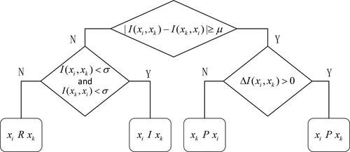
Motivated by Leik (Citation1966), we propose a consensus measure from the perspective of the frequency distribution of discrete options. The consensus degrees are measured based on the differences of binary relation types. Firstly, Example 1 shows the connection between a partial ranking and corresponding binary relations.
Example 1.
Suppose that there is a partial ranking as shown in , that is, is prefer to
and
is indifferent to
and
are prefer to
and
is incomparable to
The corresponding binary relations can be shown in .
Figure 2. An illustrative example of a partial ranking.
Source: created by the authors.
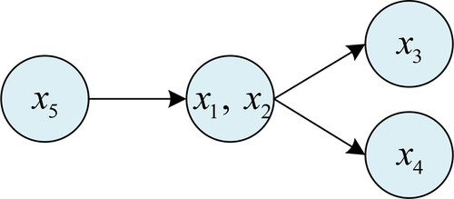
Table 3. Implicit binary relations in the illustrative partial ranking.
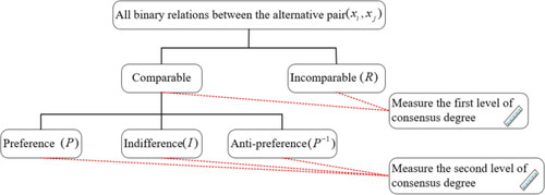
For alternatives, a total of
alternative pairs are involved. Specific to each pair, different relation types may occur according to different individual partial rankings. We can compute the consensus degree of a group according to the differences of binary relation types. The consensus measurement process has two hierarchies (see ). The binary relations are first classified into comparable relations and incomparable relations. As per the frequency distribution of these two types, the first level of consensus degree is computed. Then, the comparable relations are further classified into
and
As per the frequency distribution of these three types, the second level of consensus degree is computed.
Figure 3. A consensus measurement process in terms of two hierarches.
Source: created by the authors.
The concrete measuring process incorporated with the HFL-ORESTE method is as follows. Suppose that all experts’ final partial rankings are obtained from the HFL-ORESTE method. For each alternative pair, there are binary relations. Assume that we collect
relations between the alternative pair
and construct to measure the first level of consensus degree.
Table 4. The frequency distribution of the relation types between in the first level.
Focusing on the comparable relations, we further establish to measure the second level of consensus degree.
Table 5. The frequency distribution of the relation types between in the second level.
From and , we have and
The method based on the frequency distribution is free of the number of options and the distances between adjacent options. However, the orders of options make sense. Here, with only two options is a special case, but the option orders in must be
or
where
and
are two extreme relations and
is between
and
Considering the weight vector of experts, in , the effective frequency of a relation from the partial ranking of expert
is computed by
(7)
(7)
In , the effective frequency of a relation from the partial ranking of expert is computed by
(8)
(8)
where
is the normalised weight when only considering the experts whose relation types are comparable. Concretely, suppose that the total weight of the experts whose relation types are comparable is
Then, we have
(9)
(9)
Afterwards, for both and , a dissimilarity degree of the option is computed by
(10)
(10)
where
is the cumulative relative frequency of the
option as listed in and .
Let be the number of options. A normalised result is further obtained by
(11)
(11)
where
denotes the maximum of the sum of the dissimilarity degrees, reflecting the maximum dispersion. The maximum dispersion occurs when half of the assessments are in each of two extreme options, respectively. In this case, for
options, the dissimilarity degree vector
is
Hence, a general formula for computing
is inferred as:
(12)
(12)
For with two options, represents the maximum dispersion. By EquationEquation (12)
(12)
(12) , we have
For with three options,
and
represent the maximum dispersion. By EquationEquation (12)
(12)
(12) , we have
By EquationEquation (11)(11)
(11) ,
is a ratio scale variable in the form of percentage. With that, the ordinal consensus degree is defined as:
(13)
(13)
We have The closer the value of
is to 1, the higher the consensus degree is. By EquationEquations (10)–(13), for binary relations between the alternative pair
the two levels of consensus degrees are obtained as
and
To combine these two levels, a weighted averaging process is required. Because
based on omits the differences in the comparable parts and
based on omits the differences in the incomparable parts, the weight vector
is used, such that
(14)
(14)
In this way, the ordinal consensus degree can be computed for the opinions under each alternative pair. To check whether the consensus degrees are acceptable, a consensus threshold should be set. When a new consensus measure is proposed, there is no previous experience to refer to. Therefore, it is motivated for us to develop a method to determine the corresponding consensus threshold.
4.2. A consensus threshold determination method close to cognitive expression
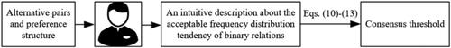
Generally, the consensus threshold is set by the decision-maker who acts as the organiser of the decision-making process and invites experts to evaluate alternatives. For different problems, the decision-maker has different acceptable consensus levels. Taking the majority voting rule as an example, the decision-maker may express the acceptable consensus level as: 3/4 of the experts agree with a scheme. The core problem of the threshold determination is how to transform the acceptable consensus level into the consensus degree that matches the corresponding consensus measure. Namely, the decision-maker’s cognitive expression should be clearly reflected in the threshold. Regarding our proposed consensus measure, the acceptable consensus level can be expressed by depicting the frequency distribution tendency. The train of thinking to set the threshold is shown in .
Figure 4. The train of thinking to set the consensus threshold.
Source: created by the authors.
Although both and
are in the interval
the measurement of
is based on two relation types while the measurement of
is based on three. Different numbers of options mean different dispersion chance. For instance, when there are only two options, the dispersion chance is little. In this case, the dispersion should be punished a lot. That is, in the case of only two options, the same dispersion can result in a lower consensus degree than in the case of more than two options. Therefore, the thresholds for
and
are different. In this sense, the determination of the global consensus threshold should also be divided into two hierarchies, and then a weighted averaging process like EquationEquation (14)
(14)
(14) is required.
For the first hierarchy of consensus threshold back to the corresponding measurement process, only two options (comparable relation and incomparable relation) are involved. Therefore, the ideal frequency distribution tendency is easy to describe. For example, the decision-maker can express the acceptable consensus level as: 90% of the relations should be in the same type and only 10% are allowed to be in the opposite type. Then, by EquationEquations (10)–(13),
is obtained.
For the second hierarchy of consensus threshold three options (
and
) are involved. In this regard, the description of the acceptable frequency distribution tendency needs to be divided into two cases:
Most relations are
Most relations are
By EquationEquations (10)–(13), the thresholds in both cases are calculated and takes the maximum of the two.
Finally, the global consensus threshold is computed by
(15)
(15)
It should be noted that the consensus thresholds for different alternative pairs may be different because of the different weight vectors in EquationEquation (15)(15)
(15) .
4.3. A consensus improving process
After the consensus measurement and the threshold determination, we check whether the consensus degree is acceptable. If for
the consensus state among individual partial rankings is acceptable; otherwise, experts should discuss and make necessary preference (criterion value) modifications towards a point of consensus. To advise experts on preference modifications, in this part, we develop a feedback mechanism compatible with the proposed consensus measure.
Let individual partial rankings be denoted by binary relation matrices where
Let the collective partial ranking be denoted by
where
In the binary relation matrices, we have
and
Hence, we use the upper triangular elements of matrices as a simple representation, i.e.,
for
Generally, to form a local feedback strategy (Wu & Xu, Citation2018) in the feedback mechanism, identification rules can help identify the preference values and the experts in need of modifications, direction rules can indicate modification directions. In this study, the identification rules are designed as follows:
Rule 1-1: Identify the alternative pairs where the binary relation types need to be modified. The alternative pairs with unacceptable consensus degrees are identified as:
(16)
(16)
Rule 1-2: Identify the experts who should modify preferences. Concretely, the identified experts are supposed to modify their assessments of and
As a result, in the experts’ partial rankings, the binary relations between
and
can change to improve the ordinal consensus level. In this part, we do not apply the axiomatic distance between relations (Jabeur et al., Citation2004; Jabeur & Martel, Citation2010) to identify the expert
whose relation type
is far from the collective one
Instead, we further conduct the consensus measurement process to indicate the consensus level of the expert
compared with the collective opinions. Concretely, let the relative frequency of
be equal to the weight of
Then, the collective opinions are treated as the opinions of everyone except
to measure differences. Namely, the relative frequency of
is
After constructing the frequency distribution table, by EquationEquations (10)–(13), the consensus degree
is obtained. Here, we measure the type differences between individual result
and the collective result
If both
and
are comparable, the second level of consensus degree is the result; otherwise, we measure the first level of consensus degree. Namely, the weighted averaging process as EquationEquation (14)
(14)
(14) is not required. The experts with poor consensus level should be identified. Generally, we select the expert with the lowest consensus level by
(17)
(17)
Labella et al. (Citation2020) claimed that consensus measures based on the distances from individual opinions to the collective opinions and the distances between individual opinions are both important. Here, the measurement is based on the type differences between the individual result and the collective result
In Section 4.1, the measurement is based on the type differences between all individual results. In this way, both the consensus measures mentioned by Labella et al. (Citation2020) are involved in this study.
Moreover, if there are multiple experts with the lowest consensus level, and the consensus state does not require a lot of modifications, we can further compare the experts along the following lines. For if we replace
with
and the transitivity of the partial ranking of expert
is still satisfied or least affected, then
should be selected. Because in this case, the modifications of
towards the collective opinions are natural. Here, we clarify the transitivity of partial rankings. Due to the conflict analyses in the ORESTE method in this study, only the
relation in partial rankings has the transitivity (hereafter called the
transitivity), i.e.,
for
Obviously, the
transitivity always holds if the replacement only involve the
and
relations. Hence, if
and
then
which means that the experts whose modifications do not affect the
transitivity should be identified; otherwise, let
be a variable, denoting the number of non-transitive cases after replacing
with
and let
which identify the experts whose modifications have the least impact on the
transitivity.
The pseudocode for the above further identification procedure is given as follows:
The further identification procedure of experts based on transitivity
Input: The identified alternative pair the relation matrices
(
)
Output: The identified expert set
Initialisation:
for
if
for
else if the
After the identification, we find that the expert should modify the assessments about
and
in the HFL decision matrix
Then, the direction rules are obtained by comparing the individual preference score
with the collective score
Rule 2-1: If (
),
should decrease the criterion value
Rule 2-2: If (
),
should increase the criterion value
Note. The preference score and the criterion value are inversely proportional.
With the feedback suggestions, the experts discuss and reappraise relevant alternatives. Then, a new consensus level is measured. In this sense, the ordinal CRP is iterative.
5. An illustrative example
In this part, the effectiveness of our method is demonstrated through an application example regarding the evaluation of design schemes in the automotive development phase. Also, comparative analyses are provided.
5.1. Problem description
The vehicle evaluation based on multiple criteria is an important activity for both the automakers and consumers (Jiang et al., Citation2018; Meng & Ding, Citation2020). Especially, in the research and development of automobile products, the evaluation and comparison of design schemes can work as references for the follow-up actions, such as production line upgrades, acquisitions, factory openings and closures. Objective and efficient evaluation enables automakers to carry out business activities economically. To be specific, the tuning of automotive chassis systems plays a crucial role in vehicle comfort and handling (Karimi Eskandary et al., Citation2016). The automotive chassis involves four subsystems: transmission, driving, steering and braking. In the development phase, different design schemes are developed by tuning the fundamental parameters in the subsystems, such as spring stiffness, damping characteristics of shock absorbers, suspension geometry, wheel alignment and brake-pedal travel. Then, the design schemes need to be evaluated. Concretely, the vehicle evaluation can be based on objective criteria that do not require drivers’ participation and feedback. For example, the maximum speed and braking distance can be obtained by experiments or simulations. However, the subjective feelings of drivers cannot be ignored in many evaluation criteria (Jiang et al., Citation2018), such as the steering response and the braking stability. Hence, automakers usually invite consumers and opinion leaders in the automotive sector to evaluate and compare different design schemes under multiple criteria. In this sense, the evaluation is an MCGDM problem. Concrete binary relations between design schemes can help automakers to conduct subsequent analyses. Given that the HFLTS is useful in depicting qualitative automotive performances, the HFL-ORESTE method is applicable. A collective decision that meets the consensus requirements can be obtained by the proposed ordinal CRP.
Suppose that there are five automobile chassis design schemes where
to be compared. The evaluation criteria involve steering response (
), transient handling performance (
), braking stability (
) and curve accelerating stability (
). The corresponding criterion weight vector
is denoted by HFLEs. A consumer representative (
), two professional car reviewers (
), a parts design engineer (
) and a chassis engineer (
) are involved as experts in the GDM process. The corresponding expert weight vector
is
The LTS used to evaluate the criterion value is
and the LTS used to indicate the criterion weights is
Here, the criterion weight vector is determined in advance as
5.2. Solving process
As per experts’ evaluations, individual HFL decision matrices for
are obtained as follows:
Step 1: The individual selection process.
Base on EquationEquations (1)(1)
(1) and Equation(2)
(2)
(2) , the global preference scores are derived from experts’ evaluation information. Then, the average preference intensities are obtained by EquationEquations (3)
(3)
(3) and Equation(4)
(4)
(4) . We put the results in the Appendix to save space. Motivated by Liao et al. (Citation2018a), we set the HFL indifference threshold
as 0.06. On this basis, we have
and
which are used in the conflict analyses to identify binary relations between alternatives. The results are as follows:
Step 2: The preference fusing process.
By EquationEquation (6)(6)
(6) , we aggregate individual preference scores into collective preference scores and put the results in .
Table 6. The collective preference scores.
Similarly, we conduct the selection process and obtain the collective binary relation results, such that:
Step 3: The consensus reaching process.
For each alternative pair, we measure the ordinal consensus degree based on the differences of binary relation types. Taking the alternative pair () as an example, we show the consensus measurement process as follows:
By EquationEquations (7)–(9), two frequency distribution tables are constructed as and .
Table 7. The frequency distribution of the relation types between in the first level.
Table 8. The frequency distribution of the relation types between in the second level.
Table 9. The ordinal consensus degrees for
Then, two levels of ordinal consensus degrees are obtained as per EquationEquations (10)–(13), i.e., By the weighted averaging formula EquationEquation (14)
(14)
(14) , the ordinal consensus degree for the alternative pair
is
Similarly, the ordinal consensus degrees for all alternative pairs are calculated as given in .
Regarding the consensus threshold, for the first hierarchy, the automaker describes the acceptable distribution tendency as: 70% of the relations are the same type and 30% are allowed to be the opposite type. Hence, by EquationEquations (10)–(13), we have For the second hierarchy, two descriptions are given as: (1) if 60% of the relations are preference relations, 30% of the relations can show a few disagreements and 10% of the relations can be the opposite type; (2) if 60% of the relations are indifferent, 40% of the relations can show a few disagreements where in the 40% portion, half of the relations can be the opposite type. The consensus degrees in both cases are calculated and we take the maximum as the threshold, i.e.,
Finally, the global consensus threshold for each alternative pair is calculated by EquationEquation (15)
(15)
(15) and given in .
Table 10. The consensus thresholds for
Comparing with 10, the alternative pairs with unacceptable consensus degrees are identified as: Then, we measure the consensus level of each expert. For
we have
For
we have
For
we have
Accordingly, the identified expert sets are:
Comparing individual preference scores with collective scores, the modification directions are available. Finally, the feedback suggestions are provided to experts. For instance,
is suggested to increase the criterion value
and decrease the criterion value
The feedback suggestions aim at conveying the collective opinions to experts. On this basis, through discussions in the decision group,
and
reappraise the relevant alternatives and modify the preferences. Suppose that after modifications, new preferences are fed into the individual selection process. The results are as follows:
Then, after preference fusion, the new collective opinion is The new consensus degrees are
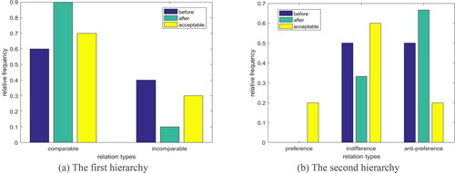
Taking
as an example, we show the changes of binary relations in .
Figure 5. The frequency variations of binary relations in
(a) The first hierarchy (b) The second hierarchy
Source: created by the authors.
The changes about the relation can result in the changes of the weight vector in EquationEquation (15)
(15)
(15) . Hence, the threshold
is updated to 0.6 and
is updated to 0.58. For all alternative pairs, the consensus degrees are acceptable. Finally,
is the collective result that meets the consensus requirement.
5.3. Comparisons
Comparative analyses are carried out from three aspects. Firstly, we explain the obtained result of our work in light of See and Lewis (Citation2006)’s research which also completed a vehicle evaluation by an MCGDM method in consideration of group consensus. Their work considered the indifference relations of alternatives but ignored the incomparability relations, and finally obtained a linear complete ranking of alternatives. Our consensus result took into account the incomparability relation and its difference with other binary relations by the proposed ordinal consensus measure. The incomparability relations of alternatives were eliminated along with the difference of opinions by the information exchange of experts in the CRP. What we obtained is also a linear complete ranking. Our method did not force an absolutely comparable or completely consensus result, but admitted the possible conflicts and tried to resolve them through information exchange, which ensured that the obtained evaluation result was objective and reasonable. Back to the vehicle evaluation problem, such an objective evaluation result can be used as an important reference for some business behaviors of automakers, such as the determination of pricing strategy and production proportion.
Secondly, we compare our ordinal consensus measure with the existing cardinal consensus measure. The cardinal consensus measure focuses on the differences between HFL information in decision matrices (Tian et al., Citation2019; Wu & Xu, Citation2018). However, different decision matrices may lead to the same ranking results. For clarification, we visualise the average preference intensities and
from five experts’ decision matrices in . The binary relations corresponding to each region are shown in .
Figure 6. The average preference intensities between and
Source: created by the authors.
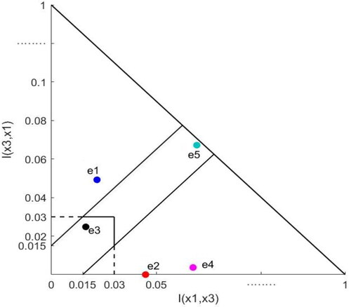
Figure 7. The schematic of conflict analysis.
Source: from Liao et al. (Citation2018a).
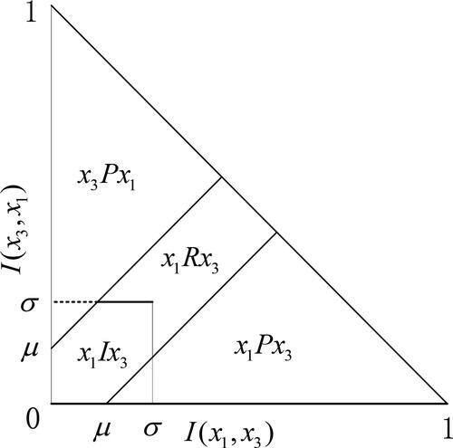
As shown in , the preference intensities of and
are different. If we use cardinal consensus measures, the distances between the opinions of the two experts are considered. However, as shown in , in the final partial ranking, the opinions of the two experts correspond to the same binary relation, i.e.,
With our ordinal consensus measure,
and
are in a unanimous agreement. The ordinal measure is robust because it only emphasises the ranking results contributing to the final decision. With the same ranking results, the differences in preference intensities cannot affect the consensus degrees. As a numerical example, we figure out the cardinal consensus degree for
i.e.,
and compare it with the ordinal one, i.e.,
Based on the preference scores of
and
the net preference intensities derived from the evaluation information of five experts are 0.0274, −0.0639, 0.0083, −0.0449, −0.0022, respectively. We normalise the preference intensities to 0, 1, 0.2092, 0.7919, 0.3242, and apply the cardinal consensus measure based on the distances among experts to obtain
The cardinal consensus degree considering preference intensities is quite different from the ordinal one based on the binary relations of alternatives.
Thirdly, we compare our ordinal consensus measure based on the differences of relation types with Jabeur and Martel (Citation2010)’s ordinal consensus measure based on the axiomatic distances between relations. The quantisation of the distance is shown in (Jabeur & Martel, Citation2010).
Figure 8. The distances between binary relations.
Source: from Jabeur et al. (Citation2004).
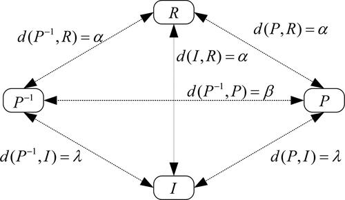
Jabeur and Martel (Citation2010) considered two preconditions: (1) (2)
Both the preconditions were correct. A neutral treatment of the
relation was implemented.
was regarded as the largest because
and
are two extreme relations. However, when assigning concrete distance values, they must further assume that
or
which was counterintuitive and non-neutral. Back to our method as indicated in , we do not put four binary relations together to measure consensus degrees. Instead, we divide the differences between partial rankings into two parts: (1) the differences between comparable and incomparable relations, (2) the differences between comparable relations
and
As per the frequencies of different relations, we measure the consensus degrees of the two parts, and then make aggregation. Hence, our proposed consensus measure is based entirely on the difference of relation types, making no assumptions about the relation itself.
6. Concluding remarks
This study applied the HFL-ORESTE method to acquire individual partial rankings and then calculated the weighted arithmetic mean of individual preference scores as the collective preferences in MCGDM. If the individual opinions differ greatly, the collective opinions as a compromise result of the weighted averaging process may be unrepresentative. To ensure the collective decision meets the consensus requirement, we designed an ordinal CRP which focused on the differences of implicit binary relation types in partial rankings. Innovatively, an enhanced consensus measure based on the frequency distribution of relation types in two hierarchies was designed. In this way, we avoided subjective axiomatic assumptions to be made about the binary relations, and the setting of the consensus threshold was intuitive. Then, we designed a corresponding feedback mechanism to conduct experts to modify preferences. The originality was that we further examined the consensus level of each expert by comparing with the collective partial ranking. Finally, the feasibility of our method was shown by an example about the evaluation of automotive design schemes. Based on the comparative analyses, it was observed that the ordinal CRP for partial rankings is effective since it only emphasises the differences in ranking results. Besides, the consensus measurement was based on a neutral treatment of the incomparability relation and free of the comparisons between the incomparability and indifference relations.
According to this research, we obtain management implications from two aspects:
When the government and organisations face decision-making problems in various economic activities, they should not force a linear complete ranking of action plans but just consider it as a signal to cease the polling of information. Allowing conflict situations to appear as incomparable relations between action plans is a rational and objective approach. The incomparable relations can be seen as a temporary compromise that requires more information and follow-up analysis.
In GDM scenarios that require group wisdom, to pursue a consensus decision, focusing on the divergence of decision-making results rather than the divergence of preferences is an efficient and economical way, which motivates the so-called ordinal consensus measure. Considering the partial rankings, it is meaningful to develop and apply an ordinal consensus measure compatible with incomparable relations in partial rankings.
There are still limitations in our work. For each alternative pair, two hierarchies of consensus degrees need to be calculated and then be aggregated into a global one. It is a heavy burden for decision-makers when there are many alternatives. Additionally, in the identification procedure of experts, we have not designed a computer program to test the transitivity. The test process can only be completed manually. In the future, the proposed consensus measure can be applied in various cases involving partial rankings. The method deserves to be extended to a large-scale GDM consensus scenario (Tang & Liao, Citation2021). Additionally, it is worth thinking whether the ordinal consensus measure based on frequency distribution is still applicable when the preference ranking is in a linguistic form (Gou et al., Citation2021). As for application cases, practical problems in the automotive industry such as partner selection (Liao et al., Citation2020) and optimisation of automotive supply chain networks (Yildizbaşi et al., Citation2018) are worth studying in the future.
Disclosure statement
No potential conflict of interest was reported by the authors.
Additional information
Funding
References
- Bouyssou, D. (1996). Outranking relations: Do they have special properties? Journal of Multi-Criteria Decision Analysis, 5(2), 99–111. https://doi.org/10.1002/(SICI)1099-1360(199606)5:2<99::AID-MCDA97>3.0.CO;2-8
- Cook, W. D. (2006). Distance-based and ad hoc consensus models in ordinal preference ranking. European Journal of Operational Research, 172(2), 369–385. https://doi.org/10.1016/j.ejor.2005.03.048
- Cook, W. D., Kress, M., & Seiford, L. (1986). Information and preference in partial orders: A bimatrix representation. Psychometrika, 51(2), 197–207. https://doi.org/10.1007/BF02293980
- Cook, W. D., & Seiford, L. (1978). Priority ranking and consensus formation. Management Science, 24(16), 1721–1732. https://doi.org/10.1287/mnsc.24.16.1721
- Di Bella, E., Gandullia, L., Leporatti, L., Montefiori, M., & Orcamo, P. (2018). Ranking and prioritization of emergency departments based on multi-indicator systems. Social Indicators Research, 136(3), 1089–1107. https://doi.org/10.1007/s11205-016-1537-5
- Gou, X. J., Xu, Z. S., Zhou, W., & Herrera-Viedma, E. (2021). The risk assessment of construction project investment based on prospect theory with linguistic preference orderings. Economic Research-Ekonomska Istraživanja, 34(1), 709–731. https://doi.org/10.1080/1331677X.2020.1868324
- Greco, S., Ishizaka, A., Tasiou, M., & Torrisi, G. (2021). The ordinal input for cardinal output approach of non-compensatory composite indicators: The PROMETHEE scoring method. European Journal of Operational Research, 288(1), 225–246. https://doi.org/10.1016/j.ejor.2020.05.036
- Herrera-Viedma, E., Cabrerizo, F. J., Kacprzyk, J., & Pedrycz, W. (2014). A review of soft consensus models in a fuzzy environment. Information Fusion, 17(1), 4–13. https://doi.org/10.1016/j.inffus.2013.04.002
- Herrera-Viedma, E., Herrera, F., & Chiclana, F. (2002). A consensus model for multiperson decision making with different preference structures. IEEE Transactions on Systems, Man, and Cybernetics - Part A: Systems and Humans, 32(3), 394–402. https://doi.org/10.1109/TSMCA.2002.802821
- Jabeur, K., & Martel, J. (2010). An agreement index with respect to a consensus preorder. Group Decision and Negotiation, 19(6), 571–590. https://doi.org/10.1007/s10726-009-9160-3
- Jabeur, K., Martel, J., & Khélifa, S. (2004). A distance-based collective preorder integrating the relative importance of the group's members. Group Decision and Negotiation, 13(4), 327–349. https://doi.org/10.1023/B:GRUP.0000042894.00775.75
- Jiang, K., Luo, Z. Q., Feng, Z. X., Huang, Z. P., & Yu, Z. H. (2018). Subjective evaluation of automobile power performance based on RA-AHP. Cognition, Technology & Work, 20(3), 413–424. https://doi.org/10.1007/s10111-018-0488-9
- Kacprzyk, J., & Fedrizzi, M. (1988). A ‘soft’ measure of consensus in the setting of partial (fuzzy) preferences. European Journal of Operational Research, 34(3), 316–325. https://doi.org/10.1016/0377-2217(88)90152-X
- Karimi Eskandary, P., Khajepour, A., Wong, A., & Ansari, M. (2016). Analysis and optimization of air suspension system with independent height and stiffness tuning. International Journal of Automotive Technology, 17(5), 807–816. https://doi.org/10.1007/s12239-016-0079-9
- Labella, Á., Ishizaka, A., & Martínez, L. (2021). Consensual group-AHPSort: Applying consensus to GAHPSort in sustainable development and industrial engineering. Computers & Industrial Engineering, 152, 107013. https://doi.org/10.1016/j.cie.2020.107013
- Labella, Á., Liu, H. B., Rodríguez, R. M., & Martínez, L. (2020). A cost consensus metric for consensus reaching processes based on a comprehensive minimum cost model. European Journal of Operational Research, 281(2), 316–331. https://doi.org/10.1016/j.ejor.2019.08.030
- Leik, R. K. (1966). A measure of ordinal consensus. The Pacific Sociological Review, 9(2), 85–90. https://doi.org/10.2307/1388242
- Liao, H. C., Li, Z. M., Zeng, X. J., & Liu, W. S. (2017). A comparison of distinct consensus measures for group decision making with intuitionistic fuzzy preference relations. International Journal of Computational Intelligence Systems, 10(1), 456–469.
- Liao, H. C., Wu, X. L., Liang, X. D., Xu, J. P., & Herrera, F. (2018a). A new hesitant fuzzy linguistic ORESTE method for hybrid multi-criteria decision making. IEEE Transactions on Fuzzy Systems, 26(6), 3793–3807. https://doi.org/10.1109/TFUZZ.2018.2849368
- Liao, H. C., Wu, X. L., Liang, X. D., Yang, J. B., Xu, D. L., & Herrera, F. (2018b). A continuous interval-valued linguistic ORESTE method for multi-criteria group decision making. Knowledge-Based Systems, 153, 65–77. https://doi.org/10.1016/j.knosys.2018.04.022
- Liao, H. C., Xue, J. F., Nilashi, M., Wu, X. L., & Antucheviciene, J. (2020). Partner selection for automobile manufacturing enterprises with a Q-rung orthopair fuzzy double normalizaion-based multi-aggregation method1. Transformations in Business and Economics, 19(2), 338–368.
- Liao, H. C., Xu, Z. S., Zeng, X. J., & Merigó, J. M. (2015). Qualitative decision making with correlation coefficients of hesitant fuzzy linguistic term sets. Knowledge-Based Systems, 76, 127–138. https://doi.org/10.1016/j.knosys.2014.12.009
- Mardani, A., Jusoh, A., Halicka, K., Ejdys, J., Magruk, A., & Ahmad, U. N. U. (2018). Determining the utility in management by using multi-criteria decision support tools: A review. Economic Research-Ekonomska Istraživanja, 31(1), 1666–1716. https://doi.org/10.1080/1331677X.2018.1488600
- Meng, F. Y., & Ding, Y. Q. (2020). An improved ELECTRE-III for recommending new energy vehicles with heterogeneous decision-making information. International Journal of Modelling, Identification and Control, 34(4), 328–341. https://doi.org/10.1504/IJMIC.2020.112298
- Morente-Molinera, J. A., Wu, X., Morfeq, A., Al-Hmouz, R., & Herrera-Viedma, E. (2020). A novel multi-criteria group decision-making method for heterogeneous and dynamic contexts using multi-granular fuzzy linguistic modelling and consensus measures. Information Fusion, 53, 240–250. https://doi.org/10.1016/j.inffus.2019.06.028
- Mousset, C. (2009). Families of relations modelling preferences under incomplete information. European Journal of Operational Research, 192(2), 538–548. https://doi.org/10.1016/j.ejor.2007.09.030
- Pastijn, H., & Leysen, J. (1989). Constructing an outranking relation with ORESTE. Mathematical and Computer Modelling, 12(10-11), 1255–1268. https://doi.org/10.1016/0895-7177(89)90367-1
- Peng, H. G., Wang, J. Q., & Zhang, H. Y. (2020). Multi-criteria outranking method based on probability distribution with probabilistic linguistic information. Computers & Industrial Engineering, 141, https://doi.org/10.1016/j.cie.2020.106318
- Rodriguez, R. M., Martinez, L., & Herrera, F. (2012). Hesitant fuzzy linguistic term sets for decision making. IEEE Transactions on Fuzzy Systems, 20(1), 109–119. https://doi.org/10.1109/TFUZZ.2011.2170076
- Roubens, M. (1982). Preference relations on actions and criteria in multicriteria decision making. European Journal of Operational Research, 10(1), 51–55. https://doi.org/10.1016/0377-2217(82)90131-X
- Roubens, M., & Vincke, P. (1985). Preference Modelling. In Lecture Notes in Economics and Mathematical Systems (250). Springer-Verlag.
- See, T. K., & Lewis, K. (2006). A formal approach to handling conflicts in multiattribute group decision making. Journal of Mechanical Design, 128(4), 678–688. https://doi.org/10.1115/1.2197836
- Sellak, H., Ouhbi, B., Frikh, B., & Ikken, B. (2019). Expertise-based consensus building for MCGDM with hesitant fuzzy linguistic information. Information Fusion, 50, 54–70. https://doi.org/10.1016/j.inffus.2018.10.003
- Shen, F., Liang, C., & Yang, Z. Y. (2021). Combined probabilistic linguistic term set and ELECTRE II method for solving a venture capital project evaluation problem. Economic Research-Ekonomska Istraživanja, 1–23. https://doi.org/10.1080/1331677X.2021.1880957
- Tang, M., & Liao, H. C. (2021). From conventional group decision making to large-scale group decision making: what are the challenges and how to meet them in big data era? A state-of-the-art survey. Omega, 100, https://doi.org/10.1016/j.omega.2019.102141
- Tang, M., Zhou, X. Y., Liao, H. C., Xu, J. P., Fujita, H., & Herrera, F. (2019). Ordinal consensus measure with objective threshold for heterogeneous large-scale group decision making. Knowledge-Based Systems, 180, 62–74. https://doi.org/10.1016/j.knosys.2019.05.019
- Tian, Z. P., Nie, R. X., Wang, J. Q., & Zhang, H. Y. (2019). Signed distance-based ORESTE for multicriteria group decision-making with multigranular unbalanced hesitant fuzzy linguistic information. Expert Systems, 36(1), e12350–24. https://doi.org/10.1111/exsy.12350
- Wu, X. L., & Liao, H. C. (2019). A consensus-based probabilistic linguistic gained and lost dominance score method. European Journal of Operational Research, 272(3), 1017–1027. https://doi.org/10.1016/j.ejor.2018.07.044
- Wu, Z. B., & Xu, J. P. (2018). A consensus model for large-scale group decision making with hesitant fuzzy information and changeable clusters. Information Fusion, 41, 217–231. https://doi.org/10.1016/j.inffus.2017.09.011
- Xu, Z. S., & Wang, H. (2017). On the syntax and semantics of virtual linguistic terms for information fusion in decision making. Information Fusion, 34, 43–48. https://doi.org/10.1016/j.inffus.2016.06.002
- Yildizbaşi, A., Çalik, A., Paksoy, T., Zanjirani Farahani, R., & Weber, G. (2018). Multi-level optimization of an automotive closed-loop supply chain network with interactive fuzzy programming approaches. Technological and Economic Development of Economy, 24(3), 1004–1028. https://doi.org/10.3846/20294913.2016.1253044
- Yoo, Y., Escobedo, A. R., & Skolfield, J. K. (2020). A new correlation coefficient for comparing and aggregating non-strict and incomplete rankings. European Journal of Operational Research, 285(3), 1025–1041. https://doi.org/10.1016/j.ejor.2020.02.027
Appendix
Table A1. The global preference scores derived from the evaluations of
Table A2. The average preference intensities derived from the evaluations of
Table A3. The global preference scores derived from the evaluations of
Table A4. The average preference intensities derived from the evaluations of
Table A5. The global preference scores derived from the evaluations of
Table A6. The average preference intensities derived from the evaluations of
Table A7. The global preference scores derived from the evaluations of
Table A8. The average preference intensities derived from the evaluations of
Table A9. The global preference scores derived from the evaluations of
Table A10. The average preference intensities derived from the evaluations of