How do social and economic factors affect carbon emissions? New evidence from five ASEAN developing countries

Abstract

This study analyzes the long and short-run impacts of social and economic factors on carbon emissions from five developing ASEAN countries during the period 1986–2017. Utilising a Pooled Mean Group Estimator, we find a nonlinear relationship between CO₂ emissions and real GDP, confirming the Environmental Kuznets Curve. Our results indicate that energy consumption is the main driver of environmental degradation in these countries; and that FDI and urbanisation reduce carbon emissions. Our research indicates both a long-run and short-run nexus between government education expenditures and CO₂ emissions. We conclude with policy suggestions to reduce CO₂ emissions while attaining sustainable growth.

Keywords:

• Carbon emissions
• GDP
• foreign direct investment
• energy consumption
• urbanisation
• government education expenditures
• Environmental Kuznets Curve
• ASEAN countries

JEL CODES:

• M4
• Q5
• R1

1. Introduction

As developing countries industrialise, economic growth increases as does environmental damage, especially so, given that modern industrialisation depends on fossil fuels (Hang & Yuan-Sheng, 2011; Kang et al., 2016; Saboori & Sulaiman, 2013). Studies indicate that carbon emissions from energy consumption in developing countries are greater than in developed countries. Moreover, policymakers in developing countries also promote per capita income via FDI inflows, providing flexible policies and lenient legal frameworks. FDI might thus be a driver of higher energy consumption (Ahmad & Du, 2017; Baek, 2016; Foon Tang, 2009). Furthermore, these nations have been urbanising at an increasing level, which increases energy use and CO₂ emissions (Hossain, 2011; Martínez-Zarzoso & Maruotti, 2011; Sadorsky, 2014). Given that environmental education has been found to increase awareness of environmental damage (Jaus, 1982; Özden, 2008), our paper will also investigate if government education expenditures reduces carbon emissions.

We investigated five ASEAN nations: Indonesia, Malaysia, Philippines, Thailand, and Vietnam during the period 1986–2017. These nations have similar socioeconomic, geographical, cultural, and environmental features. Moreover, the International Monetary Fund (IMF)¹ indicates the five are among the world’s top-20 drivers of global GDP growth. And, not surprisingly, they are facing numerous environmental challenges; indeed a recent report by IQAir Air Visual and Greenpeace indicates that these nations are among the world’s most polluted countries.

The level of carbon emissions from developing countries in the ASEAN nations has been increasing rapidly; a trend expected to continue, with Malaysia the highest, approximately 9 metric tons in recent years. For the period 2017–2018, the urban/rural ratio was 76% in Malaysia; 55%, 47% in Indonesia and Philippines, respectively, and is over 30% in Vietnam and Myanmar.

The five countries prioritise economic growth at the expense of environmental health and sustainable growth. Hence, identification of the elements responsible for increasing carbon emissions is important in order to help policymakers establish effective strategies to control CO₂ emissions.

This paper differs from the literature in the following four ways:

• The literature investigating the nexus of carbon emissions and economic growth in transitional and developing nations suffers from omitted variable bias (Mitić et al., 2017; Narayan & Narayan, 2010). While some studies have found an inverted U-shaped EKC (Al-Mulali et al., 2015; Hanif & Gago-de-Santos, 2017), others (Al-Mulali et al., 2015; Narayan & Narayan, 2010) could not find an EKC for low and low-middle income countries. Some researchers (Gökdere, 2005; Pao & Tsai, 2011; Shahbaz et al., 2013; Tang & Tan, 2015) found a relationship between carbon emissions and economic growth, foreign direct invesment (FDI), and energy; however, their results are inconclusive and mixed. Our study is the first to analyse the causal interactions between demographic, social factors, and CO₂ emissions.

• Ours is the first empirical study to include government spending in the same multivariate EKC estimation.

• Our paper highlights the dynamic impact of economic growth, energy use, FDI, urbanisation, and government education expenditures on carbon emissions in both the short-run and long-run using a Pooled Mean Group (PMG) analysis. Previous studies analysed only the long-term effects. Thus, our paper provides an effective foundation for understanding the foundational link between environmental education and CO₂ emissions.

2. Literature review

A myriad of studies have investigated the causal relationship between CO₂ emissions and economic factors, i.e., economic growth, FDI flows, and energy consumption; and social factors, such as urbanisation. However, the empirical evidence has been inconclusive.

One research stream has investigated the nexus between economic growth and the environment using the framework of the Environmental Kuznets Curve (EKC). Kuznets (1955) demonstrated an inverted-U shaped relationship between economic development and environmental degradation. The EKC theory states that carbon emissions and income increase until a turning point of income is reached, after which carbon emissions decrease.

The EKC’s inverted U-shape suggests that the process of economic growth itself will reduce CO₂ emissions once the economy matures. However, Rahman (2020), Sharif et al. (2020) and Wawrzyniak and Doryń (2020) found that economic growth leads to greater environmental degradation.

Wawrzyniak and Doryń (2020) employed GMM estimation to analyse the relationship between economic growth and CO₂ emissions, dependent on the quality of institutions (measured by a government efficiency index) from 93 emerging and developing countries during the period 1995–2014. They found evidence of decreasing emissions with an increasing GDP, which implies that EKC is supported. However, this finding is ambiguous and unreliable, as the inverted U-shaped relationship was found without time-fixed effects. The authors also argued that in nations with a strong institutional quality a GDP increasereduces environmental degradation, whereas in countries with weak institutional quality, increased GDP increases carbon emissions. Furthermore, Wawrzyniak and Doryń found that the impact of GDP on CO₂ emissions is statistically significant only where the institutional quality was lower than the average sample level.

The relationship between CO₂ emissions and economic growth has been extensively investigated in the literature of developing countries. Tamazian and Rao (2010), for example, provided supporting EKC evidence for 24 transition economies for the period 1993–2004. A quadratic nexus of income growth and CO₂ emission for China during the period 1975–2005 was found by Jalil and Mahmud (2009). However, the EKC hypothesis was not supported in other studies. Narayan and Narayan (2010) found no supporting long-run and short-run evidence for 43 developing countries. Lean and Smyth (2010) investigated five ASEAN countries during the period 1980–2006, and found that the EKC hypothesis is supported in the whole sample; however, the results vary by country (the EKC is supported in Philippines while not for other countries). Arouri et al. (2012) found a palpably different EKC turning point across a sample of Middle Eastern and North African nations during the period 1981–2005.

Several studies have documented an N-shaped curve. Churchill et al. (2018) investigated the OECD during the period 1870–2014 and found two turning points in Australia, Canada, and Japan; with Spain and the UK not following this shape. Sarkodie and Strezov (2019) also further explored the N-shape relationship for the top five emitters of greenhouse gas emissions of developing countries with panel data from 1982 to 2016 and found results confirming both the EKC framework and the N-shape. Likewise, Kang et al. (2016), and Zhou et al. (2017) demonstrated an inverted N-shaped EKC for China. Ozturk and Acaravci (2010), analysing the EKC for Turkey during the period 1968–2005, found no long-run causal relationship between CO₂ emissions and GDP per capita.

Following the seminal study of Kraft and Kraft (1978), a second stream of studies has focussed on the relationship between CO₂ emissions, economic development, and energy consumption. Scholars (Bakirtas & Akpolat, 2018; Rafindadi & Ozturk, 2017; Wang & Wang, 2020) have argued that greater economic development requires more energy consumption; similarly, energy use is efficient at a higher level of economic growth.

The synthesis of these two literature streams has fostered research linking the dynamic relationship of emissions, energy consumption, and income. Most such studies have been conducted for single countries, while some have investigated cross-country. For example, studies investigating France (Ang, 2007), and Malaysia (Ang, 2008) found that income growth is a cause of energy consumption and carbon emissions. Soytas et al. (2007), investigating the United States, obtained a reverse nexus: CO₂ emissions cause energy consumption and economic development. Niu et al. (2011) investigated eight Asia-Pacific countries, including developing countries, during the period 1971–2005, finding that energy consumption is the preponderant reason for CO₂ emissions. Additionally, they found a long-run causal linkage of CO₂ emissions and income growth, energy consumption, and emissions. However, for the short-run, they found a unidirectional causality between energy consumption and CO₂ emissions. Hanif et al. (2019), utilising an Autoregressive Distributive Lag (ARDL) model for fifteen developing Asian countries, found that economic growth increases CO₂ emissions, and fossil fuels consumption produces carbon emissions, with consequential environmental degradation.

A third stream tests the effect of financial development, proxied by foreign direct investment (FDI flows), on environmental performance. While the pollution haven hypothesis (PHH) (Jensen, 1996) states that polluting industries will be transferred to countries where environmental regulations are weak and less stringent, nevertheless, FDI enables emerging markets to utilise technological innovation, with foreign investors tending to apply a universal environmental standard. Consequently, FDI might improve the environmental quality in the host countries (Sandbroke & Mehta, 2002; Tamazian et al., 2009), or it may enhance economic growth and increase environmental degradation because profit-driven companies recognise the gap of environmental law and avoid costly environmental damage in their home nation (Dean et al., 2005; Hoffmann et al., 2005; Mujtaba et al., 2021).

Studies have also investigated the association between financial development and environmental performance, with conflicting evidence. Zhu et al. (2016) employed a panel quartile regression to test the pollution haven hypothesis for five ASEAN countries during the period 1981–2011, finding a negative nexus between FDI and carbon emissions. Acharyya (2009); Kirkulak et al. (2011); Tang and Tan (2015) rejected the PHH in India, China, and Vietnam, respectively. Behera and Dash (2017) collected data for 17 countries in South and Southeast Asia during the period 1980–2012, finding a positive relationship. More recent research (Solarin et al., 2017; To et al., 2019; Zakarya et al., 2015) found that FDI strongly impacts the environment, supporting the validity of the PHH. Atici (2012) did not find any causal relationship between FDI and CO₂ in developing ASEAN countries from 1970 to 2006; and likewise, Phuong (2018), using data from Vietnam during the period 1986–2015.

Most studies (Acheampong, 2018; Cai et al., 2018; Hanif et al., 2019; Muhammad & Khan, 2021; Munir et al., 2020) have investigated the impact of economic factors on environmental degradation. Although another possible determinant of environmental performance is social elements such as urbanisation, and the literacy rate, which has received little attention, very few researchers (Li & Lin, 2015; Pata, 2018) have included urbanisation (measured as the proportion of the urban population to the total population) in the EKC framework. Bryant (2005) found that urbanisation is related to industrialisation, technological involvement, globalisation, and migration.

Given that industrialisation usually occurs in the urban population, urbanisation can be hypothesised as a pollution source. And since industrialisation increases income levels, the demand for energy intensive products increases, causing environmental problems. Nonetheless, via awareness campaigns and stringent environmental policies, an affluent population might realise the negative impacts of environmental degradation so that environmentally friendly goods are encouraged. Furthermore, the theory of the compact city posits that urbanisation might reduce environmental damage due to economies of scale and higher population density. Therefore, urbanisation can either positively or negatively impact the environment.

The literature about the impact of urbanisation on the environment has not been resolved. For example, Cole and Neumayer (2004) utilised panel data from 86 countries and found that increased carbon emissions were followed by an increase in urbanisation. Similarly, Kasman and Duman (2015), utilising panel data of new EU members and candidate countries during the period 1992–2010, found that urbanisation has a long-run significant positive effect on CO₂ emissions. They concluded that countries with larger urban populations meet pollution standards more than countries with lower urbanisation. For 17 developed countries, Liddle and Lung (2010) found that carbon emission is insignificant in urbanised areas because the residents primarily use synthetic energy. Fan et al. (2006) proposed that urbanisation negatively affects CO₂ emissions. In a study of Malaysia, Shahbaz et al. (2016) found an inverted U-shaped for urbanisation and CO₂ emissions. They suggested that innovative technologies can help reduce energy consumption and CO₂ emissions in urban regions over the long run. Wang et al. (2021) also found an inverted U-shaped relationship between urbanisation and CO₂ emissions in OECD ountries.

Although the literature is concerned about objective influences on environmental degradation, we feel that environmental awareness is key to reducing environmental damage. Thus, promoting positive environmental awareness/attitudes is an important part of education.

Research on environmental education began during 1970s. The Tbilisi Declaration (1977) emphasised the importance of building environmental awareness and that increased awareness of the local environment is a necessary antecedent for environmental stewardship. Fisman (2005); Jaus (1982); and Mittelstaedt et al. (1999) found a positive correlation between environmental education and cognitive levels of students towards environmental issues. Several authors (Barraza & Walford, 2002; Liefländer et al., 2013; Pesaran, 2007; Zsóka et al., 2013) argue that education is necessary for students in developing and transitional countries to increase their awareness of environmental problems; and with positive attitudes towards the environment, they will become aware of environmental problems and be motivated to reduce CO₂ emissions. Gökdere (2005) suggested that we should environmentally educate at a young age.

Finally, the government’s role in environmental education is preponderant to induce beneficial changes in environmental awareness. A government’s budget may support environmental quality, particularly in emerging markets. In our study, we investigate how government education expenditures impact CO₂ emissions, the first such study in the literature.

3. Data and methodology

3.1. Data and model specification

We utilise secondary data for five ASEAN developing countries: Indonesia, Malaysia, Myanmar, Philippines, and Vietnam, for the period of 1986–2017. Table 1 reports a brief description of the variables:

Table 1. Description of the variables.

Variable	Units of measure	Definition	Sources
Carbon emissions (CO2)	Metric tons per capita	Carbon dioxide emissions are generated from burning fossil fuels and producing cement. They produce carbon dioxide emissions while using solid, liquid, and gas fuels.	The integrated Carbon Observation System-ICOS
Real GDP per capita GDP	Real GDP per capita (US$)	Nominal GDP per capita is defined as gross domestic product divided by population, measured in the middle of the year. Real GDP is nominal GDP divided by the GDP deflator^a (base year varies by country).	WDI-World Bank
Real Foreign direct investment (FDI)	Real FDI, net inflows (BoP, US$)	Foreign direct investment, also known as direct investment includes equity, income reinvestment, and other types of capital. Real FDI is measured as adjusted FDI from the GDP deflator.	WDI-World Bank
Energy Use (EU)	Kg per capita	Total kg of oil equivalent consumption per capita.	WDI-World Bank U.S. Energy Information Administration
Urban population (URB)	Percent	The percentage of urban population of the total population.	WDI-World Bank
Government expenditures for education (GOE)	Percent	The proportion of government education expenditures in total GDP.	WDI-World Bank & documents of the ministry of education of countries.

^aThe GDP deflator measures the changes in prices for all of the goods and services produced in an economy. It is calculated using the following formula: GPD deflator = Nominal GDP/Real GDP × 100.

Table 2 provides summary statistics of the variables.

Table 2. Descriptive statistics.

Variable	Mean	Std. Dev.	Min	Max
Year			1986	2017
Country			1	5
CO2	2.43	2.13	0.26	8.13
GDP	6,490.67	25,663.18	794.94	314,924.8
EU	1,017.32	743.80	260.79	3,108.82
FDI	6,770,000,000	7,170,000,000	(13,500,000,000)	49,800,000,000
URB	42.44	13.76	19.62	75.44
GOE	3.40	1.56	0.25	7.65

Source: Author’s own calculation using Stata 15. Number of observations = 160.

We extended the quadratic EKC model to examine the influence of both economic and social elements, including GDP per capita (GDP), the square of GDP per capita (GDP²), energy consumption (EU), foreign direct investment (FDI), urbanisation (URB), and government education expenditures (GOE) on the generation of carbon emissions in five ASEAN developing countries. The specified model is (1) $${\text{CO}}_{\text{2it}}{\text{ = α + β}}_{\text{1}}{\text{GDP}}_{\text{it}}{\text{+ β}}_{\text{2}}\text{GD}{P}_{it}^2 {\text{+ β}}_{\text{3}}{\text{EU}}_{\text{it}}{\text{+ β}}_{\text{4}}{\text{FDI}}_{\text{it}}{\text{+ β}}_{\text{5}}{\text{URB}}_{\text{it}}{\text{+ β}}_{\text{6}}{\text{GOE}}_{\text{it}}{\text{+ ε}}_{\text{it}}$$(1) where i, t denote the country and the time period, respectively. All variables are in natural logarithms.

As above-mentioned, there is a nonlinear inverse U-shape in the relationship between income and environmental degradation (Grossman & Krueger, 1991; Kuznets, 1955). GDP and GDP² are the traditional variables in EKC model. The threshold of GDP is calculated using the following equation: (2) $$\mathrm{GDP}\mathrm{*}=e^{\frac{{-\beta }_1}{{2\beta }_2}}$$(2)

We expect a positive sign for ${\beta }_1$ and a negative sign for ${\beta }_2,$ which supports the EKC hypothesis. Foreign direct investment and energy consumption may stimulate carbon emissions, especially in emerging and industrialising nations, with a concomitant higher demand for energy. Thus, we hypothesise the signs of ${\beta }_3$ and ${\beta }_4$ to be positive.

Although attracting foreign direct investment may bring either advantages or disadvantages for the host countries, we expect a positive sign of FDI on emissions for the following reasons:

Firstly, exporting pollution from developed countries to developing countries through FDI has been recently increasing. FDI companies have ignored waste treatment systems, and FDI projects have caused environmental pollution due to outdated technology, and a myopic overemphasis on increasing profits.

Secondly, they produce goods likely to pollute the environment such as chemicals, textiles, dyes, and tobacco. These goods are not allowed to be produced in the home country, so they go to other countries with lax environmental regulations.

Thirdly, to attract FDI, the governments of the five developing ASEAN countries have issued preferential policies and lax environmental regulations (and environmental monitoring) for foreign investors.

Finally, the FDI increase creates a challenge for ecological diversity, risking adverse effects on biodiversity, water resources, fisheries, climate, and pollution of river basins. The expansion of industrial zones has reduced forests, destroying natural habitats.

We expect the influence of social elements on the environmental quality to be statistically significant. Particularly, in developing countries, a large percent of the population is migrating from rural to urban areas. For example, the number of people in Vietnam’s largest cities increases annually, two-thirds coming from rural areas. Pollution might be increased by a growing urban population so that ${\beta }_5$ is expected to be positive. Whereas, we expect that ${\beta }_6$ is negative due to the importance of education policies and government budget supports.

3.2. Methodology

To examine the causal linkages between CO₂ emissions and the independent variables in the long-run and the short-run, our testing procedure consists of three steps. First, the panel unit root tests the order of the series. Second, if these variables are nonstationary in their level form, we utilise panel cointegration tests to determine whether the series are integrated. Then, if a cointegrating relationship exists among the variables, we apply the PMG estimator to estimate the long-run and short-run elasticities. Finally, the Granger causality test will estimate error correction models to explore the interactions in the short and long-run dynamics. Our methodology is organised as follows.

3.2.1. The cross-sectional dependence test

Before examining the panel unit root tests, we examine the cross-sectional dependence of the panel data, particularly the cross multiple regressions. Cross-sectional dependence typically leads to large standard errors, one of the reasons for biases in estimation. In our study, we test for cross-sectional dependence in panel data via three approaches: Pesaran, Friedman, and Frees.

The Pesaran test (Pesaran, 2004, 2007) is based on the LM test statistic of Breusch and Pagan (Breusch & Pagan, 1980). However, the latter doesn’t work with a large cross-sectional dimension, so a preferred alternative is the CD statistic which relies on the pair-wise correlation coefficients: $$\mathrm{CD}\mathrm{ }=\mathrm{ }\sqrt{\frac{2T}{N(N-1)}}\mathrm{ }\left(\sum _{i=1}^{N-1}\sum _{J=i+1}^N\widehat{p_{ij}}\right)$$ where T: the panel time dimension; N: the cross-sectional dimension; and u_it: error term. p_ij denotes the estimate of the pairwise correlation coefficient of the residuals: $${\rho }_{ij}={\rho }_{ji}=\mathrm{ }\frac{{\Sigma }_{t=1}^T{u}_{it}{u}_{jt}}{{\left({\Sigma }_{t=1}^T{u}_{\mathrm{i}t}^2\right)}^{\raisebox{1ex}{$1$}\!\left/ \!\raisebox{-1ex}{$2$}\right.}{\left({\Sigma }_{t=1}^T{u}_j^{2}t\right)}^{\raisebox{1ex}{$1$}\!\left/ \!\raisebox{-1ex}{$2$}\right.}}$$

Following the average rank correlation coefficient of Spearman (1906), Friedman (1937) developed a nonparametric test. The formula, developed by Frees (1995), based on the sum of squared rank correlation of the error terms, is superior to Friedman’s approach when T is large, whereas a poor Q distribution will occur with a small T.

In addition, if the panel data displays cross-sectional independence in the error terms, we must check the heterogeneous panel in order to select the appropriate unit root testing.

3.2.2. Panel unit root tests

The panel unit root test is an essential step in the process of estimation and regression. Dickey and Fuller (1979) and Fuller (1976) pioneered this in time series. Based on the traditional unit root test of Dickey-Fuller (DF) or the Augmented Dickey-Fuller (ADF), researchers have developed panel unit root tests.

In this paper, we applied the Im, Pesaran, and Shin (Im et al., 2003) test to set the order of integration of the series. This test is commonly conducted in cross-sectional independence as well as heterogeneous panels. The heterogeneous panel data model of the IPS is $${\Delta \gamma }_{it}=\mathrm{ }{\mu }_i+{\beta }_i{\gamma }_{i,t-1}+\sum _{k=1}^{{\rho }_i}{\mathrm{\varnothing }}_{i,k}{\Delta \gamma }_{i,t-k}+{\gamma }_{j}t+\mathrm{ }{\epsilon }_{it}$$

The series is stationary given an integrated series of order zero I(0); while the series is nonstationary in the level and its stationarity in the first difference given an integrated series of order one I(1).

3.2.3. Panel cointegration tests

If the results of the previous sections indicate non-stationary cross-sectional units, the cointegration test will assess the long-run relationships among the variables.

The nexus between cointegration was first suggested by Granger (1981) and Engle and Granger (1987). The cointegration tests are based on Engle and Granger’s framework. Later development of this testing included Kao (1999), Maddala and Wu (1999), Pedroni (1999, 2004), and Westerlund (2005).

The following model of cointegration tests for stationary estimated residuals: $$Y_{it}={\alpha }_i+{\lambda }_{i}t+\sum _{j=1}^m{\beta }_{ji}{X}_{ji}+\mathrm{ }{ϵ}_{it}$$ where i = 1,…,N denotes the number of cross-sectional units; t = 1,…,T is the number of observations; and m is the number of regressions.

The equation of estimated residuals is calculated by $${\epsilon }_{it}={\rho }_i{\epsilon }_{it-1}+u_i$$

Pedroni’s test is similar to Kao’s, albeit with differences: Kao tests for homokedascity across cross-sections, while Pedroni specifies cross-section intercepts and heterogenous coefficients on the first stage regression. In our paper, we also applied Westerlund’s panel cointegration test. This testing has good small sample properties along with high relative to residual–based panel cointegration tests. However, its limitation is that there is no information about the rejected cross-section.

3.2.4. Regression tests by the Pooled Mean Group estimator (PMG)

In order to estimate the long-run relationship as well as the short-run parameter estimates between variables in non-stationary panels, we construct a pooled mean group estimator (PMG), advanced by Pesaran and Smith (1995) and Pesaran et al. (1997, 1999). This technique combines pooling and averaging of coefficients. In addition, we employ two alternative models for comparison purposes: the dynamic fixed effects (DFE) estimator, relying on the pooling of cross-sections, and the mean group (MG) estimator, relying on the averaging of cross-sections.

Since all variables are I(1) and cointegrated, their principal feature is to respond to any deviation from long-run equilibrium. This implies that the short-run effects of the variables in an error correction model are influenced by the deviation from equilibrium.

Therefore, Eq. (1)(1) $${\text{CO}}_{\text{2it}}{\text{ = α + β}}_{\text{1}}{\text{GDP}}_{\text{it}}{\text{+ β}}_{\text{2}}\text{GD}{P}_{it}^2 {\text{+ β}}_{\text{3}}{\text{EU}}_{\text{it}}{\text{+ β}}_{\text{4}}{\text{FDI}}_{\text{it}}{\text{+ β}}_{\text{5}}{\text{URB}}_{\text{it}}{\text{+ β}}_{\text{6}}{\text{GOE}}_{\text{it}}{\text{+ ε}}_{\text{it}}$$(1) can be represented as an error correction equation: (3) $$\mathrm{\Delta ln}{{\mathrm{(CO}}_{\mathrm{2)}}}_{\mathrm{it}}={\varnothing }_i\left[\hspace{0.17em}\text{ln}\hspace{0.17em}{{\mathrm{(CO}}_{\mathrm{2)}}}_{\mathrm{it-1}}-{\alpha }_{\mathrm{0i}}-{\alpha }_{\mathrm{1i}}\hspace{0.17em}\text{ln}\hspace{0.17em}{\mathrm{GDP}}_{\mathrm{it}}- {\alpha }_{\mathrm{2i}}{\left(\hspace{0.17em}\text{ln}\hspace{0.17em}{\mathrm{GDP}}_{\mathrm{it}}\right)}^2- {\alpha }_{\mathrm{3i}}{\hspace{0.17em}\text{ln}\hspace{0.17em}\mathrm{EU}}_{\mathrm{it}} - {\alpha }_{\mathrm{4i}}{\hspace{0.17em}\text{ln}\hspace{0.17em}\mathrm{FDI}}_{\mathrm{it}}- {\alpha }_{\mathrm{5i}}{\hspace{0.17em}\text{ln}\hspace{0.17em}\mathrm{Urban}}_{\mathrm{it}} - {\alpha }_{\mathrm{6i}}{\hspace{0.17em}\text{ln}\hspace{0.17em}\mathrm{GOE}}_{\mathrm{it}}\right] - {\beta }_{\mathrm{11i}}\mathrm{\Delta }{\hspace{0.17em}\text{ln}\hspace{0.17em}\mathrm{GDP}}_{\mathrm{it}}-{\beta }_{\mathrm{21i}}\mathrm{\Delta }{\left({\hspace{0.17em}\text{ln}\hspace{0.17em}\mathrm{GDP}}_{\mathrm{it}}\right)}^2- {\beta }_{\mathrm{31i}}\mathrm{\Delta }{\hspace{0.17em}\text{ln}\hspace{0.17em}\mathrm{EU}}_{\mathrm{it}}- {\beta }_{\mathrm{41i}}\mathrm{\Delta }{\hspace{0.17em}\text{ln}\hspace{0.17em}\mathrm{FDI}}_{\mathrm{it} }- {\beta }_{\mathrm{51i}}\mathrm{\Delta }{\hspace{0.17em}\text{ln}\hspace{0.17em}\mathrm{Urban}}_{\mathrm{it} }- {\beta }_{\mathrm{61i}}\mathrm{\Delta }{\hspace{0.17em}\text{ln}\hspace{0.17em}\mathrm{GOE}}_{\mathrm{it} }+\mathrm{ }{\eta }_{\mathrm{it}’}$$(3)

The parameter φi is the error-correcting speed of adjustment term of lnCo2 towards its long-run equilibrium following a short-run shock.

3.2.5. Panel causality tests

Based on Granger (1969), a cointegrating relationship suggests causal linkages among the variables in one or two directions since they might be produced by a mechanism of error correction; however, it doesn’t indicate the direction of causality. To analyse the direction of causality among the variables, we employ an approach by Dumitrescu and Hurlin (2012). This test is a simple version of Granger (1969) which accepts the variance of coefficients across cross-section units and all regression models.

The regression model can be written as: $${\gamma }_{i,t}={\alpha }_i+\sum _{k=1}^k{\gamma }_i^{\left(k\right)}{y}_{i,t-k}+\sum _{k=1}^k{\beta }_i^{\left(k\right)}{x}_{i,t-k}+{\epsilon }_{i,t}\text{ i }=\mathrm{ }1,\mathrm{ }2,\mathrm{ }\dots \dots .,\mathrm{ }\mathrm{N}:\mathrm{ }\mathrm{t}=1,2,\dots .,\mathrm{T}$$ where x and y are the observations of stationary variables for N individuals in T periods. The lag orders K is assumed to be equal for all cross-section units of the panels$;\mathrm{and}\mathrm{ }{\mathrm{\alpha }}_{\mathrm{i},\mathrm{ }}{\beta }_i$ are also assumed to be fixed in the time dimension. However, the autoregressive parameters ${\gamma }_i^{(k)}$ and the regression coefficients ${\beta }_i^{(k)}$ are allowed to differ across groups.

4. Empirical results

4.1. The cross-sectional dependence test

According to the cross-sectional dependence test, we test for:

The null hypotheses H0: Cross-sectional independence; H1: Cross-sectional dependence

Table 3 reports the results of testing for cross-section dependence in the specification of random-effects (RE model).

Table 3. Cross-sectional dependence tests.

Test	Pesaran		Frees		Friedman
	CD test	p-Value	CD (Q)	p-Value	CD test	p-Value
FE model	−2.166	0.306	0.471***	0.0000	15.323***	0.0041
RE model	−1.440	0.338	0.644***	0.0000	20.014***	0.0005

Note: FE and RE are fixed effects and random effects models, respectively; and *** denotes statistical significance at the 1% level.

Source: Author's own calculation using Stata 15.

In both models, the Friedman and Frees statistics are the same; thus, we can reject the null hypothesis at 1%. Thus, there may exist at least two potential cases of dependence from the Friedman and Frees test. In contrast, the results of the Pesaran test, with P values higher than 5%, indicate that the null hypothesis is accepted, i.e., cross-section independence exists in the sample.

Obviously, the test results conflict; however, each has its advantages and disadvantages. From the test findings, we can select a well-suited approach for the causality tests. The Granger causality test would be applied for cross-sectional independence for all the coefficients of all states; while the Dumitrescu-Hurlin test is used in the sample of cross-section dependence for the differences of all coefficients across countries (Dumitrescu & Hurlin, 2012). Thus, our study uses the later test for the causality test.

4.2. Unit root test

Table 4 shows the results of the unit root test using the test of Im, Pesaran, and Shin (IPS test) for all variables in our model. In their level form, the integrated series is nonstationary, i.e., all variables have a unit root. However, they are stationary in the first difference form, I(1), in the five countries at the 1% significance level. The unit root test determines the order of integration of the series to ascertain that no variables are stationary in the second difference form (I2). Since whole samples are integrated of the same order I(1), we utilise the cointegration test to examine the existence of the long-run and short-run nexus between economic growth (GDP), energy consumption (EU), FDI, urbanisation (URB), government education expenditures (GOE), and CO₂ emissions.

Table 4. Unit root test.

Variable	At level			At first difference			Conclusion
	Lag length	Statistic	p-Value	Lag length	Statistic	p-Value
lnCO2	1	−0.7799	0.2177	1	−5.1255	0.0000	I(1)
lnGDP	1	0.0227	0.5091	1	−4.8978	0.0000	I(1)
lnGDP^2	1	0.0588	0.5234	1	−4.9305	0.0000	I(1)
lnEU	1	0.0308	0.5123	1	−4.0564	0.0000	I(1)
lnFDI	1	0.9076	0.8180	1	−4.6414	0.0000	I(1)
lnURB	1	−1.1214	0.1311	1	−2.0006	0.0227	I(1)
lnGOE	1	−0.5853	0.2792	1	−5.1699	0.0000	I(1)

Source: Author's own calculation using Stata 15.

4.3. Panel cointegration tests

The cointegration test is necessary to avoid the pseudo existence of causality or the absence of causes/effects, as well as determining the order of integration of variables. The nonstationary integrated series, at the significance level of 1%, from the unit root test increases the evidence for cointegration relationships among the variables. We employed three methods: Kao, Pedroni, and Westerlund for the cointegration test, each with the null hypothesis H0: no cointegration.

All tests (see Table 5) rejected the null hypothesis at 1% and 5%, respectively. Thus, there may be one or more cointegration nexus between them, supporting long-run as well as short-run relationships between the variables. In the next step, we use the PMG model to analyse the long-run and short-run effect of the variables.

Table 5. Cointegration tests.

	CO2	p-Value
Panel A: Kao test for cointegration
Modified Dickey-Fuller t	−3.1288***	0.0009
Dickey-Fuller t	−2.5610***	0.0052
Augmented Dickey-Fuller t	−3.2611***	0.0006
Unadjusted modified Dickey-Fuller t	−4.9505 ***	0.0000
Unadjusted Dickey-Fuller t	−3.1028***	0.0010
Panel B: Pedroni test for cointegration
Modified Phillips-Perron t	2.3279***	0.0100
Phillips-Perron t	−1.8424**	0.0327
Phillips-Perron t	−2.3795***	0.0087
Panel C: Westerlund test for cointegration
Variance ratio	4.2432***	0.0000

Note: ***, ** the rejection of the null hypothesis of no cointegration is statistically significant at 1%, and 5%.

Source: Author's own calculation using Stata 15.

4.4. Regressions

Ordinary Least Squares (OLS) estimators may bias the parameters in a cointegrated panel series. Therefore, we use the pooled mean group (PMG) estimator to analyse the short-run and long-run equilibrium nexus among the variables. We also add two alternative methods for comparison: the mean group (MG) and the dynamic fixed effects (DFE). Table 6 reports the results for all three estimators.

Table 6. Regression results.

Dependent variable lnCO2	Pooled mean group	Mean group	Dynamic fixed effects
	(1)	(2)	(3)
Long-run coefficients
lnGDP	1.561759***	7.869987	0.7518205
	(0.003)	(0.135)	(0.363)
lnGDP^2	−0.0732805***	−0.4149839	−0.0321042
	(0.01)	(0.189)	(0.498)
lnFDI	−0.0099837**	−0.0250403	−0.0076032
	(0.05)	(0.338)	(0.14)
lnEU	1.124368***	1.19761***	0.9549159***
	(0.000)	(0.006)	(0.001)
lnURB	−0.8981265***	−2.290846	−0.4315324
	(0.000)	(0.19)	(0.371)
lnGOE	−0.1856534***	0.1091391***	0.2775241***
	(0.000)	(0.006)	(0.001)
Short-run coefficients
Ec	−0.3168696***	−0.5652277***	−0.2017369***
	(0.000)	(0.000)	(0.000)
$\Delta$lnGDP	−1.474073	−3.974709	0.152219
	(0.49)	(0.2)	(0.485)
$\Delta$lnGDP^2	0.093739	0.2298088	0.0014027
	(0.456)	(0.18)	(0.906)
$\Delta$lnFDI	0.0012033	0.0010375	0.0002526
	(0.715)	(0.841)	(0.766)
$\Delta$lnGOE	−0.1071431***	−0.0843561	−0.0216129
	(0.004)	(0.228)	(0.467)
$\Delta$lnEU	0.2584798	0.1075305	0.3775917***
	(0.32)	(0.795)	(0.007)
$\Delta$lnURB	3.321958	5.035543	−0.2756571
	(0.474)	(0.349)	(0.707)
Constant	−3.670901	−32.2184	−1.652367**
	(0.000)	(0.086)	(0.03)
Hausman test	1.0000
Turning points—TNP ($US): 43158.577

Note: ** and *** denote rejection of the null hypothesis at the 5%, and 10% levels respectively.

Source: Author's own calculation using Stata 15.

The PMG estimator allows the short-term coefficients to vary across countries, while the MG estimator constrains the coefficients among countries as it is the average regression coefficients of each country. The speed of adjustment estimates suggest that the short-run dynamics significantly differ for each model (compare $\widehat{\varnothing }$= −0.31 from PMG and $\widehat{\varnothing }$= −0.56 from MG). The Hausman test was conducted to test the difference in these models. The Hausman statistic was 1.00, and is distributed χ2(2); thus, under the null hypothesis, the PMG estimator is more efficient than the MG estimator. The PMG results show a strong significance (at 1%) in the average short-run parameter estimate of lnGOE, suggesting a short-run relationship between lnGOE and lnCO₂.

The DFE estimator indicates the short-run effect of lnEU on lnCO₂ at 5% significance. However, the DFE estimator requires the short-run coefficients to be equal. Baltagi et al. (2000) demonstrated that FE models suffer a simultaneous equation bias from the endogeneity between the lagged dependent variable and the error term.

Thus, we conclude that the PMG estimator is consistent for estimating the short-run as well as long-run parameters of the impact of all independent variables on lnCO₂.

The estimations obtained from the PMG indicates the robust effect of all variables, which include real GDP (lnGDP), along with its square (lnGDP²), real FDI (lnFDI), energy consumption (lnEU), urbanisation (lnURB), and government education expenditures (lnGOE) on carbon emissions (lnCO₂).

The results displayed in Table 6 show that the coefficients of lnGDP and lnGDP² are statistically significant at the 1% level. Thus, there is a long-run relationship between economic growth and CO₂ emissions. The signs of lnGDP, lnGDP² are positive and negative, respectively. This implies an inverted U-shaped nexus between per capita income and CO₂ emissions, which in turn supports the EKC. As the relationship between environmental quality and economic growth is inverted U-shaped, there exists a turning point that implies a transition from a state of environmental degradation to one of environmental improvement. The turning point of GDP per capita, calculated from Eq. (2)(2) $$\mathrm{GDP}\mathrm{*}=e^{\frac{{-\beta }_1}{{2\beta }_2}}$$(2) is $43,158.577. After this point, the effect of economic growth on carbon emissions changes from positive to negative. It is difficult to determine the threshold income level of the turning point and the corresponding carbon emissions level (Yaduma et al., 2015). Hopefully this number will provide some guidance for developing countries that are similar to the five ASEAN countries analysed in this paper.

As Figure 1 displays, the inverted U-shaped in the relationship between economic growth and environmental degradation has three stages:

Figure 1. Environmental Kuznets curve.

Source: by the author based on analysis results.

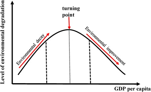
In the early stage of economic development when almost all countries were primarily based on agriculture, economic activities were less harmful to the environment. However, as nations began industrialising, industrial production expanded rapidly, exhausting natural resources and increasing environmental degradation. The after income exceeded the threshold, citizens became aware of the harmful impact of environmental degradation, thereby improving technology and reducing fossil energy use to reduce carbon emissions.

Our inverted U-shape EKC comports with Chandran and Tang (2013) and To et al. (2019). In addition, our findings indicate the impact of energy consumption on carbon emissions across models. The sign of the coefficient of energy use is positive, and specicially, a one percentage increase in energy use will increase per capita carbon emissions by 1.12 per cent. This supports our expectation that high energy use is more likely to aggravate environmental quality, and comports with the findings of Ang (2008), Ozturk and Acaravci (2010), and To et al. (2019).

Moreover, from Table 6, the coefficient of lnFDI is −0.009 at 5%, which contravenes Tang and Tan (2015) and Zhu et al. (2016) who rejected the validity of the pollution haven hypothesis. However, these results comport with To et al. (2019) who utilised data from 25 emerging markets (including our five sample nations) for the period 1980–2016. Indeed, we cannot deny benefits from FDI for developing countries. The FDI inflows transfer advanced technologies to host countries, increasing patents and domestic R&D activities. Thus, by improving productivity, increasing efficiency in input resources, energy consumption and carbon emissions could be significantly reduced.

The coefficient of lnURB is −0.89 and significant at 1%. Thus, as urbanisation increases, carbon emissions decrease, contravening our expectations. A possible explanation is the theory of the compact city, which asserts that economies of scale created by higher density urbanisation could reduce environmental damage. Moreover, more affluent people in urban areas tend to use environmental friendly products, recognising the negative impacts of environmental degradation. This comports with Shahbaz et al. (2016) who demonstrated that innovative technologies reduce energy consumption and CO₂ emissions in Malaysia’s long-run urbanisation.

It is not surprising that the sign of lnGOE is negative, with a coefficient −0.18 in long-run equilibrium at the 1% significance level. This comports with our initial expectations for the impact of government education on carbon emissions, implying that a one percentage increase in government education expenditures will mitigate carbon emissions by 0.18 per cent. Likewise, environmental education prevents environmental problems. Thus, it is important to encourage and promote a sense of environmental responsibility for children to create a positive motivation for pro-environmental behaviour through their adulthood. RecognisingR the importance of environmental education, the governments of these countries have allocated s a large amount of their budget.

In our sample, environmental education was initially conducted through extracurricular activities; later the Ministries of Education and Training of the countries added environmental education. Environmental education is conducted at all levels: pre-school, primary school, high school, colleges and universities. Environmental education strategies (lectures, school essays, environmental seminars, outdoor activities for children) are organised in accordance with cultural and traditional values. Documents, publications, textbooks, and reference books on environmental protection have been published. Media campaigns and annual contests about environmental laws have raised awareness and encouraged residents and organisations to participate in environmental protection National and international conferences, as well as environmental seminars have been organised to promote awareness, environmental knowledge, and environmental law. Moreover, environmental data has been established to manage environmental protection activities.

Indeed, environmental education helps the community understand the complex nature of natural and human-made environmental systems, producing a more friendly and understanding behaviour. Government spending on environmental education has had a positive effect on solving environmental problems and reducing CO₂ emissions.

4.5. Causality test

From the results of the above tests, particularly the cointegration relationships between variables by the cointegration test, we analyse the causal nexus between variables through pairwise directions, which ascertains the uni-directional and bi-directional causality via the Dumitrescu-Hurlin tests for panel data. We test the null hypotheses H0: Variable 1 does not cause Variable 2.

Table 7 provides the causal relationships for all variables from Eq. (1)(1) $${\text{CO}}_{\text{2it}}{\text{ = α + β}}_{\text{1}}{\text{GDP}}_{\text{it}}{\text{+ β}}_{\text{2}}\text{GD}{P}_{it}^2 {\text{+ β}}_{\text{3}}{\text{EU}}_{\text{it}}{\text{+ β}}_{\text{4}}{\text{FDI}}_{\text{it}}{\text{+ β}}_{\text{5}}{\text{URB}}_{\text{it}}{\text{+ β}}_{\text{6}}{\text{GOE}}_{\text{it}}{\text{+ ε}}_{\text{it}}$$(1) .

Table 7. Granger causality Dumitrescu-Hurlin.

Null hypothesis (H0)	W-Stat	Zbar-Stat	Prob.
lnGDP does not cause lnCO2	10.6941	9.7203	0.0000
lnCO2 does not cause lnGDP	4.5151	2.812	0.0049
lnGDP^2 does not cause lnCO2	10.7467	9.7791	0.0000
lnCO2 does not cause lnGDP^2	4.3649	2.6440	0.0082
lnEU does not cause lnCO2	13.5356	3.9057	0.0001
lnCO2 does not cause lnEU	11.0406	2.4147	0.0157
lnURB does not cause lnCO2	21.2253	8.5012	0.0000
lnCO2 does not cause lnURB	21.1759	8.4717	0.0000
lnGOE does not cause lnCO2	11.0558	3.2635	0.0011
lnCO2 does not cause lnGOE	1.2768	0.4376	0.6617
lnFDI does not cause lnCO2	16.9102	5.9225	0.0000
lnCO2 does not cause lnFDI	7.3122	9.9805	0.0686

Source: Author's own calculation using Stata 15.

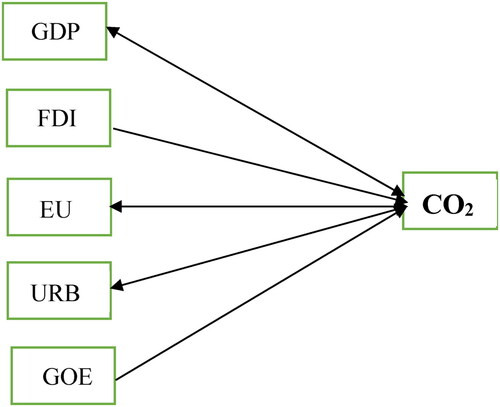
The results indicate that the bi-directional causality relationship occurs in pairs of variables: lnGDP and lnCO₂; lnGDP² and lnCO₂; lnEU and lnCO₂, lnURB and lnCO₂. This rejects the null hypothesis at the 1% significance level.

Additionally, Table 7 indicates unidirectional causality for the pair of variables lnFDI and lnCO₂. Our evidence suggests that the independent variable (lnFDI) causes lnCO₂ at the 1 significance level. The null hypothesis of no causal nexus between lnCO₂ and the independent variable (lnFDI) is accepted, implying existence of a one-way effect from lnFDI to lnCO₂.

Moreover, we also found evidence of the uni‐directional causality between lnGOE and lnCO₂. The null hypothesis that the independent variable (lnGOE) does not cause lnCO₂ is rejected at 1%; thus, lnGOE has a one-way impact on lnCO₂. However, there is not enough evidence to reject the null hypothesis of the causal relationship between lnCO₂ and the independent variables; hence lnCO₂ does not cause lnGOE.

Based on these test findings, all variables have a causal relationship with carbon emissions, supporting the regression results in Table 6.

Figure 2 summarises the causal relationships between the main variables:

Figure 2. Summary of the long‐run causality test.

Source: by the author based on analysis results.

5. Conclusions

Our findings:

• The results based on the PMG estimator reveal a nonlinear inverted U-shaped relationship between real GDP and carbon emissions, which supports the traditional EKC curve. This implies carbon emissions increase with economic growth up to a critical point, and then decrease.

• Energy consumption is the main factor of the rapid environmental degradation in the five nations of our sample. Indeed, environmental challenges in the ASEAN countries are caused by energy consumption in order to boost economic growth. This suggests that reducing energy consumption will reduce CO₂ emissions and improve environmental quality.

• A negative relationship between carbon emissions and FDI, meaning that FDI inflows could reduce carbon emissions. Policymakers are aware of environmental problems in these nations, so they have established strict regulations and standards for FDI enterprises in order to limit CO₂ emissions while ensuring sustainable growth.

• The impact of urbanisation on carbon emissions was found to be significantly negative in the long-run, but insignificant in the short-run.

• The effect of government education expenditures on improving environmental quality in both the long-run and short-run is highly significant. Obviously, government spending to reform environmetal education, particularly integrating environmental education in schools, changes the attitudes of school children towards environmental problems. They tend to be more responsible for controlling pollution and preventing harmful environmental actions. Our findings support (Lopez & Palacios, 2010) who found a relationship between government spending and environmental quality. They documented that the level and the composition of government expenditure in social and public policies is important to reduce environmental degradation.

• The empirical evidence from the Dumitrescu-Hurlin approach provides the bidirectional causality relationships among the four variables: GDP, energy consumption, urbanisation, and carbon emissions. Hence, any strategy involving one would influence the others.

Our findings allow us to offer recommendations regarding current environmental challenges for policymakers. In essence, reducing CO₂ emissions requires the monitoring of energy efficiency, choosing sustainable growth by applying advanced technology, high-performance equipment, clean and renewable energy. Moreover, today, environmental issues and climate change not only concern individual nations but also is a common regional and global concern. Thus, enhancing ASEAN member states cooperation is essential. The solutions need to be flexible, effective, and suitable to the social and economic conditions of each nation. Encourage the ASEAN nations to participate in common efforts to enhance an ASEAN Climate Change Initiative (ACCI), promote technology transfer, exchange knowledge on R&D activities, and improve the ability to adapt and mitigate the potential effects of environmental degradation. Furthermore, we believe (and supported byu the evidence produced in this paper) that environmental education is vital in addressing environment issues to sustainably develop. Governments should advocate citizen awareness programs for children and adults in order to increase the use of environmentally friendly products, helping them understand the harmful effects of a high carbon economy. Last but not least, learning from the successful experience of Singapore, an ASEAN nation, environment education along with establishing good behaviour and habits are necessary to protect the environment. The governments also need to promulgate and enforce stricter regulations pertaining to destructive environmental actions.

Given this line of discussion, there is an emphasis that the EKC hypothesis support evidence of a relationship between environmental quality and economic growth. It represents a cycle of environmental development going through different stages of industrialisation.

Developing countries are currently facing common problems including increasing energy consumption, urbanisation, attracting FDI inflows, a sufficient education budget, environmental issues, and economic development. An extended multivariate model helps examine the impact of these factors on the level of environmental degradation. Hence, it provides more quantitative scientific evidence for policymakers for making appropriate macroeconomic strategies.

6. Limitations of the study and suggested future research

Although our research makes a practical contribution to literature, its limitation needs to be considered. In this paper, we use three approaches: MG, PMG, and dynamic fixed effect (DFE) estimators for comparison. However, the outcome of the pooled mean group (PMG) estimator is used for explaining the impact of variables on CO₂ emissions in the short and long term. The PMG estimator accepts parameters in the short-run to vary freely across cross-sections, although in this case with a quadratic EKC model, the long-run coefficients may have nonlinear restrictions since the long-run coefficient is a nonlinear function of the short-run coefficients, implies that the long-run estimation might be biased when removing the bias in the short-run. The results of the unit root test suggested by, Pesaran and Shin (IPS test) indicated that all variables in our model are stationary in the first difference form. It can be assumed that the existence of a long-run relationship in the whole sample since estimation in this study was conducted. We believe it is reasonable to use the PMG estimator when estimating equations for a small number of groups (five countries).

Notwithstanding the unresolved problem in the long-run coefficients, to our knowledge, this paper will be the first to investigate the impacts of government education spending on CO₂ emissions in the EKC model. The outcome of this paper can open many new research opportunities regarding government expenditure or education elements. In future research, scholars can examine whether the literacy level of residents lead to their behaviour towards environmental problems. In line with this study, we consider how the quantity of state budget for environmental education between urban and rural affects the attitudes as well as awareness on environment. In the same way as our research, authors also suggest expanding the scope of countries that have similar socioeconomic, geographical, cultural, and environmental features in other regions of the world.

Disclosure statement

No potential conflict of interest was reported by the authors.

Notes

1 https://theaseanpost.com/article/asean-pushing-global-gdp-growth

References

- Acharyya, J. (2009). FDI, growth and the environment: Evidence from India on CO2 emission during the last two decades. Journal of Economic Development, 34(1), 43.
- Acheampong, A. O. (2018). Economic growth, CO2 emissions and energy consumption: What causes what and where? Energy Economics, 74, 677–692. https://doi.org/10.1016/j.eneco.2018.07.022
- Ahmad, N., & Du, L. (2017). Effects of energy production and CO2 emissions on economic growth in Iran: ARDL approach. Energy, 123, 521–537. https://doi.org/10.1016/j.energy.2017.01.144
- Al-Mulali, U., Weng-Wai, C., Sheau-Ting, L., & Mohammed, A. H. (2015). Investigating the environmental Kuznets curve (EKC) hypothesis by utilizing the ecological footprint as an indicator of environmental degradation. Ecological Indicators, 48, 315–323. https://doi.org/10.1016/j.ecolind.2014.08.029
- Ang, J. B. (2007). CO2 emissions, energy consumption, and output in France. Energy Policy, 35(10), 4772–4778. https://doi.org/10.1016/j.enpol.2007.03.032
- Ang, J. B. (2008). Economic development, pollutant emissions and energy consumption in Malaysia. Journal of Policy Modeling, 30(2), 271–278. https://doi.org/10.1016/j.jpolmod.2007.04.010
- Arouri, M. E. H., Ben Youssef, A., M'henni, H., & Rault, C. (2012). Energy consumption, economic growth and CO2 emissions in Middle East and North African countries. Energy Policy, 45, 342–349. https://doi.org/10.1016/j.enpol.2012.02.042
- Atici, C. (2012). Carbon emissions, trade liberalization, and the Japan–ASEAN interaction: A group-wise examination. Journal of the Japanese and International Economies, 26(1), 167–178. https://doi.org/10.1016/j.jjie.2011.07.006
- Baek, J. (2016). A new look at the FDI–income–energy–environment nexus: Dynamic panel data analysis of ASEAN. Energy Policy, 91, 22–27. https://doi.org/10.1016/j.enpol.2015.12.045
- Bakirtas, T., & Akpolat, A. G. (2018). The relationship between energy consumption, urbanization, and economic growth in new emerging-market countries. Energy, 147, 110–121. https://doi.org/10.1016/j.energy.2018.01.011
- Baltagi, B. H., Griffin, J. M., & Xiong, W. (2000). To pool or not to pool: Homogeneous versus heterogeneous estimators applied to cigarette demand. Review of Economics and Statistics, 82(1), 117–126. https://doi.org/10.1162/003465300558551
- Barraza, L., & Walford, R. A. (2002). Environmental education: A comparison between English and Mexican school children. Environmental Education Research, 8(2), 171–186. https://doi.org/10.1080/13504620220128239
- Behera, S. R., & Dash, D. P. (2017). The effect of urbanization, energy consumption, and foreign direct investment on the carbon dioxide emission in the SSEA (South and Southeast Asian) Region). Renewable and Sustainable Energy Reviews, 70, 96–106. https://doi.org/10.1016/j.rser.2016.11.201
- Breusch, T. S., & Pagan, A. R. (1980). The Lagrange multiplier test and its applications to model specification in econometrics. Review of Economic Studies, 47(1), 239. https://doi.org/10.2307/2297111
- Bryant, C. (2005). The impact of urbanisation on rural land. http://www.eolss.net
- Cai, Y., Sam, C. Y., & Chang, T. (2018). Nexus between clean energy consumption, economic growth and CO2 emissions. Journal of Cleaner Production, 182, 1001–1011. https://doi.org/10.1016/j.jclepro.2018.02.035
- Chandran, V. G. R., & Tang, C. F. (2013). The impacts of transport energy consumption, foreign direct investment and income on CO2 emissions in ASEAN-5 economies. Renewable and Sustainable Energy Reviews, 24, 445–453. https://doi.org/10.1016/j.rser.2013.03.054
- Churchill, S. A., Inekwe, J., Ivanovski, K., & Smyth, R. (2018). The environmental Kuznets curve in the OECD: 1870–2014. Energy Economics, 75, 389–399. https://doi.org/10.1016/j.eneco.2018.09.004
- Cole, M. A., & Neumayer, E. (2004). Examining the impact of demographic factors on air pollution. Population and Environment, 26(1), 5–21. https://doi.org/10.1023/B:POEN.0000039950.85422.eb
- Dean, J. M., Lovely, M. E., & Wang, H. (2005). Are foreign investors attracted to weak environmental regulations? Evaluating the evidence from China. The World Bank.
- Dickey, D. A., & Fuller, W. A. (1979). Distribution of the estimators for autoregressive time series with a unit root. Journal of the American Statistical Association, 74(366a), 427–431.
- Dumitrescu, E. I., & Hurlin, C. (2012). Testing for Granger non-causality in heterogeneous panels. Economic Modelling, 29(4), 1450–1460. https://doi.org/10.1016/j.econmod.2012.02.014
- Engle, R. F., & Granger, C. W. J. (1987). Co-integration and error correction: Representation, estimation, and testing. Econometrica, 55(2), 251–276. https://doi.org/10.2307/1913236
- Fan, Y., Liu, L.-C., Wu, G., & Wei, Y.-M. (2006). Analyzing impact factors of CO2 emissions using the STIRPAT model. Environmental Impact Assessment Review, 26(4), 377–395. https://doi.org/10.1016/j.eiar.2005.11.007
- Fisman, L. (2005). The effects of local learning on environmental awareness in children: An empirical investigation. The Journal of Environmental Education, 36(3), 39–50. https://doi.org/10.3200/JOEE.36.3.39-50
- Foon Tang, C. (2009). Electricity consumption, income, foreign direct investment, and population in Malaysia: new evidence from multivariate framework analysis. Journal of Economic Studies, 36(4), 371–382. https://doi.org/10.1108/01443580910973583
- Frees, E. W. (1995). Assessing cross-sectional correlation in panel data. Journal of Econometrics, 69(2), 393–414. https://doi.org/10.1016/0304-4076(94)01658-M
- Friedman, M. (1937). The use of ranks to avoid the assumption of normality implicit in the analysis of variance. Journal of the American Statistical Association, 32(200), 675–701. https://doi.org/10.1080/01621459.1937.10503522
- Fuller, W. A. (1976). Introduction to statistical time series. John Wiley.
- Gökdere, M. (2005). A study on environmental knowledge level of primary students in Turkey. Asia-Pacific Forum on Science Learning and Teaching, 6(2), 1–13.
- Granger, C. W. J. (1969). Investigating causal relations by econometric models and cross- spectral methods. Econometrica, 37(3), 424–438. https://doi.org/10.2307/1912791
- Granger, C. W. J. (1981). Cointegrating variables and error correcting models. University of California.
- Grossman, G. M., & Krueger, A. (1991). Environmental impacts of the North American free trade agreement. https://www.nber.org/papers/w3914
- Hang, G., & Yuan-Sheng, J. (2011). The relationship between CO2 emissions, economic scale, technology, income and population in China. Procedia Environmental Sciences, 11, 1183–1188. https://doi.org/10.1016/j.proenv.2011.12.178
- Hanif, I., & Gago-de-Santos, P. (2017). The importance of population control and macroeconomic stability to reducing environmental degradation: An empirical test of the environmental Kuznets curve for developing countries. Environmental Development, 23, 1–9. https://doi.org/10.1016/j.envdev.2016.12.003
- Hanif, I., Raza, S. M. F., Gago-de-Santos, P., & Abbas, Q. (2019). Fossil fuels, foreign direct investment, and economic growth have triggered CO2 emissions in emerging Asian economies: Some empirical evidence. Energy, 171, 493–501. https://doi.org/10.1016/j.energy.2019.01.011
- Hoffmann, R., Lee, C., Ramasamy, B., & Yeung, M. (2005). FDI and pollution: A granger causality test using panel data. Journal of International Development, 17(3), 311–317. https://doi.org/10.1002/jid.1196
- Hossain, M. S. (2011). Panel estimation for CO2 emissions, energy consumption, economic growth, trade openness and urbanization of newly industrialized countries. Energy Policy, 39(11), 6991–6999.
- Im, K., Pesaran, H., & Y. Shin, (2003). Testing for Unit Roots in Heterogeneous Panels. Journal of Econometrics, 115, 53–74. https://doi.org/10.1016/S0304-4076(03)00092-7
- Jalil, A., & Mahmud, S. F. (2009). Environment Kuznets curve for CO2 emissions: A cointegration analysis for China. Energy Policy, 37(12), 5167–5172. https://doi.org/10.1016/j.enpol.2009.07.044
- Jaus, H. H. (1982). The effect of environmental education instruction on children’s attitudes toward the environment. Science Education, 66(5), 689–692. https://doi.org/10.1002/sce.3730660504
- Jensen, V. (1996). The pollution haven hypothesis and the industrial flight hypothesis: Some perspectives on theory and empirics. University of Oslo, Centre for Development and the Environment.
- Kang, Y.-Q., Zhao, T., & Yang, Y.-Y. (2016). Environmental Kuznets curve for CO2 emissions in China: A spatial panel data approach. Ecological Indicators, 63, 231–239. https://doi.org/10.1016/j.ecolind.2015.12.011
- Kao, C. (1999). Spurious regression and residual-based tests for cointegration in panel data. Journal of Econometrics, 90(1), 1–44. https://doi.org/10.1016/S0304-4076(98)00023-2
- Kasman, A., & Duman, Y. S. (2015). CO2 emissions, economic growth, energy consumption, trade and urbanization in new EU member and candidate countries: A panel data analysis. Economic Modelling, 44, 97–103. https://doi.org/10.1016/j.econmod.2014.10.022
- Kirkulak, B., Qiu, B., & Yin, W. (2011). The impact of FDI on air quality: Evidence from China. Journal of Chinese Economic and Foreign Trade Studies, 4(2), 81–98. https://doi.org/10.1108/17544401111143436
- Kraft, J., & Kraft, A. (1978). On the relationship between energy and GNP. The Journal of Energy and Development, 401–403. http://www.jstor.org/stable/24806805.
- Kuznets, S. (1955). Economic growth and income inequality. American Economic Review, 45(1), 1–28.
- Lean, H. H., & Smyth, R. (2010). CO2 emissions, electricity consumption and output in ASEAN. Applied Energy, 87(6), 1858–1864. https://doi.org/10.1016/j.apenergy.2010.02.003
- Li, K., & Lin, B. (2015). Impacts of urbanization and industrialization on energy consumption/CO2 emissions: Does the level of development matter? Renewable and Sustainable Energy Reviews, 52, 1107–1122. https://doi.org/10.1016/j.rser.2015.07.185
- Liddle, B., & Lung, S. (2010). Age-structure, urbanization, and climate change in developed countries: Revisiting STIRPAT for disaggregated population and consumption-related environmental impacts. Population and Environment, 31(5), 317–343. https://doi.org/10.1007/s11111-010-0101-5
- Liefländer, A. K., Fröhlich, G., Bogner, F. X., & Schultz, P. W. (2013). Promoting connectedness with nature through environmental education. Environmental Education Research, 19(3), 370–384. https://doi.org/10.1080/13504622.2012.697545
- Lopez, R. E., & Palacios, A. (2010). Have government spending and energy tax policies contributed to make Europe environmentally cleaner? No. 1667-2016-136345. ageconsearch.umn.edu
- Maddala, G. S., & Wu, S. (1999). A comparative study of unit root tests with panel data and a new simple test. Oxford Bulletin of Economics and Statistics, 61(s1), 631–652. https://doi.org/10.1111/1468-0084.61.s1.13
- Martínez-Zarzoso, I., & Maruotti, A. (2011). The impact of urbanization on CO2 emissions: Evidence from developing countries. Ecological Economics, 70(7), 1344–1353. https://doi.org/10.1016/j.ecolecon.2011.02.009
- Mitić, P., Ivanović, O. M., & Zdravković, A. (2017). A cointegration analysis of real gdp and CO2 emissions in transitional countries. Sustainability, 9(4), 568. https://doi.org/10.3390/su9040568
- Mittelstaedt, R., Sanker, L., & VanderVeer, B. (1999). Impact of a week-long experiential education program on environmental attitude and awareness. Journal of Experiential Education, 22(3), 138–148. https://doi.org/10.1177/105382599902200306
- Muhammad, B., & Khan, M. K. (2021). Foreign direct investment inflow, economic growth, energy consumption, globalization, and carbon dioxide emission around the world. Environmental Science and Pollution Research International, 28(39), 55643–55654.
- Mujtaba, A., Jena, P. K., & Joshi, D. P. P. (2021). Growth and determinants of CO2 emissions: Evidence from selected Asian emerging economies. Environmental Science and Pollution Research International, 28(29), 39357–39369.
- Munir, Q., Lean, H. H., & Smyth, R. (2020). CO2 emissions, energy consumption and economic growth in the ASEAN-5 countries: A cross-sectional dependence approach. Energy Economics, 85, 104571. https://doi.org/10.1016/j.eneco.2019.104571
- Narayan, P. K., & Narayan, S. (2010). Carbon dioxide emissions and economic growth: Panel data evidence from developing countries. Energy Policy, 38(1), 661–666. [Database] https://doi.org/10.1016/j.enpol.2009.09.005
- Niu, S., Ding, Y., Niu, Y., Li, Y., & Luo, G. (2011). Economic growth, energy conservation and emissions reduction: A comparative analysis based on panel data for 8 Asian-Pacific countries. Energy Policy, 39(4), 2121–2131. https://doi.org/10.1016/j.enpol.2011.02.003
- Özden, M. (2008). Environmental awareness and attitudes of student teachers: An empirical research. International Research in Geographical and Environmental Education, 17(1), 40–55. https://doi.org/10.2167/irgee227.0
- Ozturk, I., & Acaravci, A. (2010). CO2 emissions, energy consumption and economic growth in Turkey. Renewable and Sustainable Energy Reviews, 14(9), 3220–3225. https://doi.org/10.1016/j.rser.2010.07.005
- Pao, H.-T., & Tsai, C.-M. (2011). Multivariate Granger causality between CO2 emissions, energy consumption, FDI (foreign direct investment) and GDP (gross domestic product): Evidence from a panel of BRIC (Brazil, Russian Federation, India, and China) countries. Energy, 36(1), 685–693. https://doi.org/10.1016/j.energy.2010.09.041
- Pata, U. K. (2018). Renewable energy consumption, urbanization, financial development, income and CO2 emissions in Turkey: Testing EKC hypothesis with structural breaks. Journal of Cleaner Production, 187, 770–779. https://doi.org/10.1016/j.jclepro.2018.03.236
- Pedroni, P. (1999). Critical values for cointegration tests in heterogeneous panels with multiple regressors. Oxford Bulletin of Economics and Statistics, 61(S1), 653–670. https://doi.org/10.1111/1468-0084.61.s1.14
- Pedroni, P. (2004). Panel cointegration: Asymptotic and finite sample properties of pooled time series tests with an application to the PPP hypothesis. Econometric Theory, 20(03), 597–625. https://doi.org/10.1017/S0266466604203073
- Pesaran, M. H. (2007). A simple panel unit root test in the presence of cross-section dependence.Journal of applied econometrics,22(2), 265–312. https://doi.org/10.1002/jae.951
- Pesaran, M. H. (2004). General diagnostic tests for cross section dependence in panels (Cambridge Working Papers in Economics No. 0435). University of Cambridge, Faculty of Economics.
- Pesaran, M. H., Shin, Y., & Smith, R. P. (1997). Estimating long-run relationships in dynamic heterogeneous panels (DAE Working Papers Amalgamated Series 9721). University of Cambridge, England.
- Pesaran, M. H., Shin, Y., & Smith, R. P. (1999). Pooled mean group estimation of dynamic heterogeneous panels. Journal of the American Statistical Association, 94(446), 621–634. https://doi.org/10.1080/01621459.1999.10474156
- Pesaran, M. H., & Smith, R. (1995). Estimating long-run relationships from dynamic heterogeneous panels. Journal of Econometrics, 68(1), 79–113. https://doi.org/10.1016/0304-4076(94)01644-F
- Phuong, N. D. (2018). The relationship between foreign direct investment, economic growth and environmental pollution in vietnam: An autoregressive distributed lags approach. International Journal of Energy Economics and Policy, 8(5), 138–145.
- Rafindadi, A. A., & Ozturk, I. (2017). Impacts of renewable energy consumption on the German economic growth: Evidence from combined cointegration test. Renewable and Sustainable Energy Reviews, 75, 1130–1141. https://doi.org/10.1016/j.rser.2016.11.093
- Rahman, M. M. (2020). Environmental degradation: The role of electricity consumption, economic growth and globalisation. Journal of Environmental Management, 253, 109742. https://doi.org/10.1016/j.jenvman.2019.109742
- Saboori, B., & Sulaiman, J. (2013). CO2 emissions, energy consumption and economic growth in Association of Southeast Asian Nations (ASEAN) countries: A cointegration approach. Energy, 55, 813–822. https://doi.org/10.1016/j.energy.2013.04.038
- Sadorsky, P. (2014). The effect of urbanization on CO2 emissions in emerging economies. Energy Economics, 41, 147–153. https://doi.org/10.1016/j.eneco.2013.11.007
- Sandbroke, R., & Mehta, P. (2002). FDI and environment–Lessons from the mining sector [Rapporteurs Report from the OECD Global Forum on International Investment], Paris.
- Sarkodie, S. A., & Strezov, V. (2019). Effect of foreign direct investments, economic development and energy consumption on greenhouse gas emissions in developing countries. Science of the Total Environment, 646, 862–871.
- Shahbaz, M., Hye, Q. M. A., Tiwari, A. K., & Leitão, N. C. (2013). Economic growth, energy consumption, financial development, international trade and CO2 emissions in Indonesia. Renewable and Sustainable Energy Reviews, 25, 109–121. https://doi.org/10.1016/j.rser.2013.04.009
- Shahbaz, M., Loganathan, N., Muzaffar, A. T., Ahmed, K., & Jabran, M. A. (2016). How urbanization affects CO2 emissions in Malaysia? The application of STIRPAT model. Renewable and Sustainable Energy Reviews, 57, 83–93. https://doi.org/10.1016/j.rser.2015.12.096
- Sharif, A., Godil, D. I., Xu, B., Sinha, A., Khan, S. A. R., & Jermsittiparsert, K. (2020). Revisiting the role of tourism and globalization in environmental degradation in China: Fresh insights from the quantile ARDL approach. Journal of Cleaner Production, 272, 122906. https://doi.org/10.1016/j.jclepro.2020.122906
- Solarin, S. A., Al-Mulali, U., Musah, I., & Ozturk, I. (2017). Investigating the pollution haven hypothesis in Ghana: An empirical investigation. Energy, 124, 706–719. https://doi.org/10.1016/j.energy.2017.02.089
- Soytas, U., Sari, R., & Ewing, B. T. (2007). Energy consumption, income, and carbon emissions in the United States. Ecological Economics, 62(3-4), 482–489. https://doi.org/10.1016/j.ecolecon.2006.07.009
- Spearman, C. (1906). Footrule’for measuring correlation. British Journal of Psychology, 1904-1920, 2(1), 89–108. https://doi.org/10.1111/j.2044-8295.1906.tb00174.x
- Tamazian, A., Chousa, J. P., & Vadlamannati, K. C. (2009). Does higher economic and financial development lead to environmental degradation: Evidence from BRIC countries. Energy Policy, 37(1), 246–253. https://doi.org/10.1016/j.enpol.2008.08.025
- Tamazian, A., & Rao, B. B. (2010). Do economic, financial and institutional developments matter for environmental degradation? Evidence from transitional economies. Energy Economics, 32(1), 137–145. https://doi.org/10.1016/j.eneco.2009.04.004
- Tang, C. F., & Tan, B. W. (2015). The impact of energy consumption, income and foreign direct investment on carbon dioxide emissions in Vietnam. Energy, 79, 447–454. https://doi.org/10.1016/j.energy.2014.11.033
- To, A. H., Ha, D. T.-T., Nguyen, H. M., & Vo, D. H. (2019). The impact of foreign direct investment on environment degradation: Evidence from emerging markets in Asia. International Journal of Environmental Research and Public Health, 16(9), 1636. https://doi.org/10.3390/ijerph16091636
- Wang, Q., & Wang, S. (2020). Is energy transition promoting the decoupling economic growth from emission growth? Evidence from the 186 countries. Journal of Cleaner Production, 260, 120768. https://doi.org/10.1016/j.jclepro.2020.120768
- Wang, W.-Z., Liu, L.-C., Liao, H., & Wei, Y.-M. (2021). Impacts of urbanization on carbon emissions: An empirical analysis from OECD countries. Energy Policy, 151, 112171. https://doi.org/10.1016/j.enpol.2021.112171
- Wawrzyniak, D., & Doryń, W. (2020). Does the quality of institutions modify the economic growth-carbon dioxide emissions nexus? Evidence from a group of emerging and developing countries. Economic Research-Ekonomska Istraživanja, 33(1), 124–144. https://doi.org/10.1080/1331677X.2019.1708770
- Westerlund, J. (2005). New simple tests for panel cointegration. Econometric Reviews, 24(3), 297–316. https://doi.org/10.1080/07474930500243019
- Yaduma, N., Kortelainen, M., & Wossink, A. (2015). The environmental Kuznets curve at different levels of economic development: A counterfactual quantile regression analysis for CO2 emissions. Journal of Environmental Economics and Policy, 4(3), 278–303. https://doi.org/10.1080/21606544.2015.1004118
- Zakarya, G. Y., Mostefa, B., Abbes, S. M., & Seghir, G. M. (2015). Factors affecting CO2 emissions in the BRICS countries: A panel data analysis. Procedia Economics and Finance, 26, 114–125. https://doi.org/10.1016/S2212-5671(15)00890-4
- Zhou, Z., Ye, X., & Ge, X. (2017). The impacts of technical progress on sulfur dioxide Kuznets curve in China: A spatial panel data approach. Sustainability, 9(4), 674. https://doi.org/10.3390/su9040674
- Zhu, H., Duan, L., Guo, Y., & Yu, K. (2016). The effects of FDI, economic growth and energy consumption on carbon emissions in ASEAN-5: Evidence from panel quantile regression. Economic Modelling, 58, 237–248. https://doi.org/10.1016/j.econmod.2016.05.003
- Zsóka, Á., Szerényi, Z. M., Széchy, A., & Kocsis, T. (2013). Greening due to environmental education? Environmental knowledge, attitudes, consumer behavior and everyday pro-environmental activities of Hungarian high school and university students. Journal of Cleaner Production, 48, 126–138. https://doi.org/10.1016/j.jclepro.2012.11.030