Individualism and tax progressivity

Abstract

This article proposes a novel theoretical model that factors in individualism culture for explaining tax progressivity. It shows that an increase in the level of individualism reduces optimal tax progressivity, regardless of whether a social planner or voters choose income tax schedule. Moreover, an increase in the pre-tax income inequality raises tax progressivity optimal for the social planner or voters, for any given level of individualism. These findings from introducing individualism culture for tax progressivity are quite original. This article makes an important contribution of providing an explanation for the puzzling fact that taxes of some countries with low inequality of pre-tax income are more progressive than those of other with high inequality. This article implies that a country with low pre-tax income inequality can have highly progressive tax if the country’s culture features fairly low level of individualism. Empirical analysis with panel data of 87 countries finds evidence supportive of these theoretical findings.

Keywords:

• tax progressivity
• pre-tax income inequality
• individualism culture

JEL CODE:

• D31
• H21
• H23
• H24

1. Introduction

Whether higher pre-tax income inequality entails more progressive tax is a fundamental issue of economics. It is important not only for public finance but also for macroeconomics with the unresolved controversy on whether higher pre-tax income inequality hurts economic growth by entailing more redistributive tax (e.g., Barro, 2000; Persson & Tabellini, 1994). Although optimal income taxation literature implies that higher pre-tax income inequality calls for more progressive tax to redistribute more, a lot of empirical studies (e.g., Perotti, 1996; Persson, 1995; Slemrod & Bakija, 2000) found that higher pre-tax income inequality does not entail more progressive tax. For example, pre-tax income inequality is lower in Scandinavian countries than in the US, while tax is more progressive in Scandinavian countries than in the US. This inconsistency between theoretical prediction of optimal income taxation literature and the empirical findings is puzzling and suggests that, besides pre-tax income inequality, there can be another factor playing a significant role in shaping tax progressivity. To account for this puzzling fact, we newly introduce the cultural factor of individualism. Tax of a country is a part of the country’s laws which can be affected by the country’s culture. Moreover, since tax is addressing income differences among individuals, a country’s culture about individual differences can be relevant to the country’s decision of income tax rates. Thus, this article analyses effects of individualism culture and pre-tax income inequality, respectively, on tax progressivity.

This article characterises optimal degree of tax progressivity of the entire income tax schedule in a model where each individual cares about comparing himself with others of the society that he belongs to by internalising the society’s average consumption level in their own utility. In particular, utility function of each individual of a society contains the individualism-culture parameter that indicates how much weights each individual puts on the society average.

From this model that explicitly embeds individualism culture into utility function, we first characterise socially optimal tax progressivity that a benevolent social planner obtains from maximising the social welfare (population-weighted sum of the utility of all individuals who have different earning abilities). As the social welfare also factors in the individualism culture of the society, the social planner’s optimal tax progressivity reflects the individualism culture. From the obtained formula for the social planner’s optimal tax progressivity, effect of individualism culture and pre-tax income inequality, respectively, on socially optimal tax progressivity is identified. An increase in the level of individualism leads the social planner to choose less progressive tax, for any given level of pre-tax income inequality. When individuals put a smaller weight on comparing them with others of the same society, smaller welfare gains are obtained from more progressive tax, as individuals more appreciates their uniqueness or difference from others. For any given level of individualism, an increase in the level of pre-tax income inequality raises the social planner’s optimal tax progressivity, confirming the logical inference from the optimal nonlinear income taxation literature.

Furthermore, for reflecting the reality that tax progressivity is set by policymakers who are politically motivated and thus follow voters’ decision, this article also characterises politically optimal tax progressivity that is selected by voters under the majority-rule voting. In particular, voters’ optimal tax progressivity is derived from utility maximisation of a pivotal decisive voter who turns out to be the median voter whose earning ability is the median of the earning-ability distribution. From the obtained formula for the voters’ optimal tax progressivity, which is different from the social planner’s, how individualism culture and pre-tax income inequality, respectively, affect politically optimal tax progressivity is identified. While an increase in the level of individualism reduces the politically optimal tax progressivity under the majority-rule voting, an increase in the level of pre-tax income inequality raises it. When the median voter becomes less concerned about gaps between him and the society’s average, an increase in the degree of tax progressivity brings smaller utility gains to the median voter, for any given level of pre-tax income inequality. For any given level of individualism, when pre-tax incomes become more unequal, more progressive tax brings larger utility gains to the median voter, although he does not seek social-welfare gain from redistribution. These theoretical findings of this article are robust to a change in the distribution of earning ability as well as to a change in decision mechanism from dictatorship of a benevolent social planner to democratic majority-rule voting.

While the effect of pre-tax income inequality on optimal tax progressivity (whether for voters or the social planner) remains positive regardless of the given level of individualism, it can be counteracted by an increase in the level of individualism. The theoretical findings of this article imply that an economy of low pre-tax income inequality can have highly progressive tax if the level of individualism of the economy is substantially low. This article implies that we can find statistically insignificant correlations between observed pre-tax income inequality and observed tax progressivity, as the previous empirical studies found (e.g., Perotti, 1996; Persson, 1995). That is, by the innovation of introducing the individualism culture in the model for optimal income tax progressivity, this article rationalises the puzzling fact that some countries with low pre-tax income inequality have more progressive tax than other countries with high inequality of pre-tax income. This article’s findings of pre-tax income inequality and tax progressivity are important for better understanding the relation of pre-tax income inequality and economic growth. Notably, this article suggests the need to consider the overlooked factor of individualism culture for analysing how pre-tax income inequality affects economic growth.

Lastly, the theoretical findings regarding the effects of individualism culture and pre-tax income inequality on tax progressivity are tested with panel data of 87 countries around the world between 1990 and 2005. With controlling for other economic and institutional relevant factors for tax progressivity, regression analyses are conducted and find statistically significant evidence that the effect of individualism on tax progressivity is negative while the effect of pre-tax income inequality on tax progressivity is positive. Furthermore, the econometrical analyses find that when omitting one of the two variables of pre-tax income inequality and individualism from the regression, the estimated effect of pre-tax income inequality (or individualism) on tax progressivity loses statistical significance, highlighting the need to consider the two variables together for properly identifying their respective effects on tax progressivity.

This article is organised as follows. Section 2 reviews related literature. Section 3 describes the model, from which optimal tax progressivity is characterised and the effect of pre-tax income inequality and individualism culture, respectively, on optimal tax progressivity is analysed in Sections 4 and 5. Section 6 conducts empirical analyses to test the theoretical findings. Section 7 concludes the article.

2. Literature review

First of all, from the optimal income taxation literature (e.g., Mirrlees, 1971; Werning, 2007) that justifies distortionary income taxation for addressing a given level of pre-tax income inequality, we can infer that higher pre-tax income inequality leads to more progressive tax. A larger pre-tax gap in marginal utility between the rich and the poor resulting from higher pre-tax inequality makes more progressive tax welfare-improving. Corroborating this logical inference, numerical simulations of Kanbur and Tuomala (1994) found that optimal marginal income tax rate increases with income (i.e., tax is progressive) only if pre-tax inequality is high, although Kanbur and Tuomala (1994) did not provide a theoretical proof for this finding from their simulation. As mentioned above, many empirical studies (e.g., Perotti, 1996; Persson, 1995; Slemrod & Bakija, 2000) have found that real data of pre-tax income inequality and tax progressivity do not corroborate the logical inference from the optimal income taxation literature. Above all, the existing studies in the optimal income taxation literature overlooked the factor of culture. By analysing pre-tax income inequality and optimal income tax progressivity with factoring in individualism culture, this article contributes to the literature on optimal income taxation.

As a matter of fact, with Ramsey models or Mirrleesian models that are the main workhorse models in the public finance literature, whether higher pre-tax income inequality entails more progressive tax is not easily tractable for a theoretical analysis, as acknowledged by previous studies (e.g., Kanbur & Tuomala, 1994). So far, in the optimal nonlinear income taxation literature, a clear proof for the association of pre-tax income inequality and tax progressivity is not shown. The most difficult obstacle is to formally prove a change in the progressivity of the entire income tax schedule as a result of higher pre-tax income inequality or higher level of individualism culture. To overcome the obstacle, this article utilises a widely adopted and empirically verified nonlinear income tax function that has a tractable representation of the progressivity of the entire income tax schedule.

Furthermore, the optimal income taxation literature assumes that income tax schedules are determined by a benevolent social planner, whereas actual income tax schedules are set by policymakers who follow voters’ decision, not by a social planner. In this light, by positing that tax rate is linear and chosen by voters, Meltzer and Richard (1981) showed that higher pre-tax income inequality entails higher rate of linear income tax (flat tax); however, higher flat tax rate does not mean more progressive tax. While tax progressivity depends on the slope of entire marginal income tax rate schedule, the slope is fixed under linear tax (flat tax). Thus, linear income taxation is not proper for analysing tax progressivity, as it does not allow marginal tax rates to vary across different levels of pre-tax incomes. As a matter of fact, to date, there is no theoretical study that analyses effect of pre-tax income inequality on voters’ choice of tax progressivity.

Moreover, this article makes contribution for the literature on taxation and culture (e.g., Alm & Torgler, 2006; Andriani et al., 2022; Eugster & Parchet, 2019; Guerra & Harrington, 2022; Tsakumis et al., 2007; Wynter & Oats, 2018; Yong & Martin, 2016). In fact, most of the literature of taxation and culture focused on the effect of culture on tax morale/compliance of a given income tax schedule, not on decisions of tax schedule or tax progressivity. Interpreting region-specific characteristic as culture, Eugster and Parchet (2019) analysed tax competition, while Wynter and Oats (2018) examined tax administrators’ behaviour. On the other hand, as culture has many dimensions, only some papers of the literature (e.g., Tsakumis et al., 2007; Yong & Martin, 2016) analysed effect of individualism culture on tax morale/compliance. Above all, so far, effect of individualism culture on tax progressivity is not yet analysed. Thus, this article also contributes to the literature on taxation and culture by analysing how individualism culture affects tax progressivity.

3. The economic environment

Consider an economy populated by a continuum of individuals who are differentiated by their own earning ability. Earning ability of each individual is exogenously given and represents labour productivity. In particular, earning ability $\theta \in [1,\infty )$ is distributed¹ following a Pareto distribution of $\mathit{Pareto}(\alpha )$ with $\alpha >2$ and the cumulative distribution function (C.D.F.) of $F_{\theta }.$ As a result, pre-tax incomes also follow a Pareto distribution, as shall be shown below. As well known, Pareto distribution is the most widely adopted in the optimal income taxation literature. Later, as a robustness check, the same theoretical analysis will be conducted with a Lognormal distribution, in the place of a Pareto distribution, because Lognormal distribution is also widely adopted for studies on income distributions. The population size of this economy is one. The utility function of an individual is: (1) $$v(c,l)=(1-\frac{1}{\gamma })\hspace{0.17em}\log \hspace{0.17em}(c)-\frac{l_{}^{1+\eta }}{1+\eta }+\chi \hspace{0.17em}\log \hspace{0.17em}(G)-\frac{1}{\gamma }\log \hspace{0.17em}\left(\frac{C}{c}\right)$$(1) where $c>0$ and $l\in [0,1]$ are private goods consumption and labour supply, respectively, of the individual; $G>0$ is public goods provided by the government of this economy; and, $C={\int }_1^{\infty }c(\theta )d{F}_{\theta }$ is the average private goods consumption of this economy. The parameter of $\chi >0$ represents relative preference for public goods; and, $\frac{1}{\eta }>0$ is Frisch elasticity of labour supply. As each individual is atomic, he takes the average private consumption $C$ as given.

The parameter $\gamma >1$ indicates the level of individualism culture of this economy. If the value of $\gamma$ goes to infinity, then the utility function of (1) will become a typical utility function which stipulates that individuals does not pay any attention to others in the same society at all in their decision-making. In fact, Akerlof (1997) described this highest level of individualism as ‘methodological individualism,’ because it is analytically tractable to be utilised as typical methods for economic analyses. At this highest level of individualism, each individual cares about his consumption only and does not care about comparing himself with others at all so that he is completely free from any concern on gap between his own consumption and others’ in the same society. In this extremely individualistic society, utility from consumption of an individual is completely self-reliant and independent from others’ in the same society. As opposed to individualism culture, people in collectivism culture are concerned of gap between themselves and others’ in the same society, as the value of their own consumption is not fully self-reliant but dependent of others in the same society. In collectivism culture, people often define the value of their own consumption in comparison with the society average, whereas in individualism culture, people usually find the value of their own consumption intrinsically in terms of itself as well as independent of others. Thus, if $1<\gamma <\infty$ (i.e., not at the highest level of individualism), then each individual cares about comparing himself and others in the same society and minds the gap between his own consumption with others’ to some degree. In this light, $\frac{1}{\gamma }$ can represent cultural weight that an individual puts on everyone else in the same society. If the value of $\gamma$ is low (i.e., low level of individualism), then individuals are highly concerned about the gap between their own consumption and everyone else’ consumption $C$ in the same society, as appears in the last term of (1). As others’ consumption directly enters the utility function of an individual through the last term, it exerts externality to the individual. Apparently, decision on tax rate is social decision, as it affects all individuals of an economy. As Akerlof (1997) claimed, for better understanding social decisions, it is useful to model possible others’ influence, or externality, into the utility function of an individual. Notice that this utility function is clearly different from utility functions in the literature on social status concern (e.g., Corneo, 2002; Ireland, 2001; Persson, 1995) as their utility functions depicted how an individual cares about his own social rank in their models. Their utility functions exhibited different kinds of externality to represent relative rank of an individual. Obviously, ranking is not part of the utility function of (1), and the average consumption of the society $C$ plays a role of a social reference point for an individual based on which an individual can value the difference between ‘I’ versus ‘we’ (or the society). Moreover, private goods in this model do not represent social rank of those who consume them. On the other hand, when restating (1) as $\hspace{0.17em}\log \hspace{0.17em}(c)-\frac{l_{}^{1+\eta }}{1+\eta }+\chi \hspace{0.17em}\log \hspace{0.17em}(G)-\frac{1}{\gamma }\log \hspace{0.17em}(C),$ the utility function takes a similar form of utility adopted by the articles on ‘Keeping up with the Joneses’ (e.g., Ljungqvist & Uhlig, 2000). Because the society average consumption is represented by consumption of ‘the Joneses’ and higher value of $\gamma$ means that an individual cares less about keeping up with ‘the Joneses,’ the parameter of $\gamma$ still can indicate the level of individualism in their contexts as well. Notably, the existing papers on ‘Keeping up with the Joneses’ have not analysed tax progressivity.

To clearly identify the effect of individualism culture on tax progressivity, this article inevitably needs to specify utility function and earning-ability distribution, which might not attain the highest level of generality. Nonetheless, except for the part of individualism externality in the last term of utility function, the utility function of (1) is very widely accepted in a lot of theoretical and empirical studies and receives empirical supports. To be consistent with empirical findings on labour supply behaviour, consumption utility is represented by logarithm function so that substitution and income effect of wages are approximately of the same size (Chetty, 2006; Kimball & Shapiro, 2008). Moreover, as mentioned above, Pareto distribution and Lognormal distribution are the most widely adopted by researchers, as they well approximate actual income distributions.

The government of this economy imposes income tax to finance public goods provision. In particular, the government implements a nonlinear income tax schedule that takes the following form of nonlinear tax function: (2) $$T(y)=y-\lambda y^{1-\tau }$$(2) where $T(y)$ is income tax payment from individuals whose pre-tax income is $y.$ The parameter $\tau$ represents the degree of tax progressivity, which will be further explained below. While $\tau$ captures the slope of marginal tax rate schedule, the parameter $\lambda$ does the average level of tax rate. Notably, the nonlinear tax function of (2) has been adopted by various studies such as Feldstein (1969), Benabou (2000, 2002), Corneo (2002), Heathcote et al. (2014, 2017) and the like. Furthermore, the nonlinear tax function of (2) is shown to be remarkably well fitted to the data of the US tax system (Heathcote et al., 2017).

Admittedly, in the optimal nonlinear income taxation literature, Mirrleesian model (Mirrlees, 1971) is more usual than the nonlinear tax function of (2). However, Mirrleesian model is not suitable for the present analysis, because it is usually impossible for Mirrleesian model to definitely identify progressivity of the entire income tax schedule. As proven by Diamond (1998), optimal marginal income tax rate schedule from a Mirrleesian model is U-shaped; thus, the slope of Mirrleesian income tax schedule takes negative and positive signs over different part of the schedule, which makes it impossible to definitely determine progressivity of the entire income tax schedule. In contrast, progressivity of the entire income tax schedule is consistently identifiable by $\tau$ in (2), as shall be elaborated below. Moreover, unlike the nonlinear tax function of (2), Mirrleesian income tax schedules are not empirically plausible (Mankiw et al., 2009). With the tax function of (2), theoretical analysis of how tax progressivity of the entire income tax schedule responds to higher pre-tax income inequality or to higher level of individualism becomes feasible, while it is not feasible under Mirrlees model.

Notice that post-tax income $y-T(y)$ is $\lambda y^{1-\tau }$ all of which is used for private consumption. This implies $\lambda >0$ due to $c>0.$ Furthermore, because pre-tax income is $y=\theta l$ for any given $\theta ,$ if $1-\tau \le 0$ with $\lambda >0,$ an increase in labour supply entails a decrease in the post-tax income $\lambda y^{1-\tau }.$ Thus, if $1-\tau \le 0$ with $\lambda >0,$ more labour supply does not return more disposable income for private consumption, giving individuals no incentive to work. Thus, to make individuals supply labour and earn positive amount of taxable income, (3) $$1-\tau >0 \text{and}\lambda >0.$$(3)

Importantly, notice that $\tau$ indicates progressivity of the entire income tax schedule. In particular, tax is progressive if $\tau >0$ since marginal tax rate increases with pre-tax income for $\forall y$ if $\frac{dT\prime (y)}{dy}$ $=\lambda \tau (1-\tau )y^{-\tau -1}>0$ for $\forall y.$ By the same token, tax is regressive (i.e., marginal tax rate decreases with pre-tax income for $\forall y$) if $\tau <0.$ In addition, if $\tau =0,$ income tax rate is flat and the constant marginal tax rate of $1-\lambda$ is imposed equally for all different levels of pre-tax income. Thus, the higher $\tau$ is, the steeper the slope of the entire income tax schedule is. At the same time, note that average income tax rate $\frac{T(y)}{y}$ is lower (higher) than marginal income tax rate $T\prime (y)$ if $\tau >0$ ($\tau <0$).

When the government chooses a nonlinear income tax schedule, it should meet the following budget constraint: (4) $$G=gY={\int }_1^{\infty }T(y(\theta ))d{F}_{\theta }$$(4) where $Y$ is total output of this economy and $g\in (0,1)$ is exogenously given portion of total output earmarked for public goods provision. Moreover, while public goods are perfectly substitutable with private goods to be final consumption goods as numeraire of this economy, public goods can be provided only by the government. Since the focus of this article is not on public goods provision, $g$ is treated as a given parameter as in many previous studies on optimal income taxation.² In fact, even when g is endogenously chosen by the government, the results of this article are not changed. Most of all, for any given $g,$ $\tau$ uniquely defines $\lambda$ that meets the budget constraint of (4). That is, $\lambda$ is automatically determined, once $\tau$ is chosen. Although the slope of marginal tax rate schedule $\tau$ alone cannot define the level of tax, with the government budget constraint of (4), the level of the schedule is defined by determining the value of $\lambda .$ As such, $\lambda$ represents the average level of tax rate. In addition, an increase in $\tau$ (tax progressivity) under the balanced budget entails an increase in $\lambda$ to meet the budget constraint of (4). As the portion of output used for public goods provision is given, extra tax revenue resulting from an increase in $\tau$ is absorbed by an increase in $\lambda$ to keep the budget balance.

As in most of studies on optimal nonlinear income taxation, there is a representative firm that produces final consumption goods according to linear production technology using labour: (5) $$Y={\int }_1^{\infty }\theta ld{F}_{\theta }.$$(5)

At a competitive equilibrium of this economy, profit of the representative firm is maximised yielding zero profit to yield zero economic profit and factor market is cleared to equate market wage rate with earning ability (labour productivity). Thus, for any given $\theta ,$ pre-tax income of an ability-$\theta$ individual is $\theta l;$ and, according to (2), post-tax income of an ability-$\theta$ individual is $\lambda {(\theta l)}^{1-\tau }.$ For any given $\theta ,$ an ability-$\theta$ individual maximises his utility subject to his own budget constraint of $c\le \lambda {(\theta l)}^{1-\tau }.$

For any given income tax schedule ($\tau$ and $\lambda$) and $g,$ a competitive equilibrium of this economy is attained if: (i) the allocation decision rules of ${\{c(\theta ),\mathrm{ }l(\theta )\}}_{\theta =1}^{\infty }$ maximise the utility of each individual meeting their own budget constraint; (ii) the profit of the representative firm is maximised, and factor market is cleared by equating wage rate with marginal labour product (earning ability); and (iii) the government budget is balanced. According to Walras’ law, once this economy reaches its competitive equilibrium, the following aggregate resource constraint is automatically met, clearing goods market as well: (6) $$Y=C+G.$$(6)

To set a benchmark, we first let a benevolent social planner dictate income tax schedule ($\tau$ and $\lambda$). Then, to reflect the reality that income tax schedule is decided by policymakers who follow voters’ decision, we later let income tax schedule ($\tau$ and $\lambda$) be decided by majority-rule voting of all individuals of this economy. Regardless of how income tax schedule is decided, allocation of private consumption and labour supply is decided by individuals themselves and implemented through competitive markets. Thus, optimal income tax schedule should be supported as a competitive equilibrium, regardless of whether it is chosen by voters or the social planner.

With their own individuals’ utility being maximised, all of the post-tax income is used for private consumption so that their budget constraint is binding; hence, $c=\lambda y^{1-\tau }=\lambda {(\theta l)}^{1-\tau }$ for any given $\theta$ at a competitive equilibrium of this economy. Thus, each individual maximises $v(\lambda {(\theta l)}^{1-\tau },l)=\hspace{0.17em}\log \hspace{0.17em}(\lambda {(\theta l)}^{1-\tau })-\frac{l_{}^{1+\eta }}{1+\eta }+\chi \hspace{0.17em}\log \hspace{0.17em}(G),$ whose first-order condition yields (7). When plugging (7) into $\lambda {(\theta l)}^{1-\tau }$ entails (8). Thus, competitive-equilibrium allocation $\{c(\theta ),\mathrm{ }l(\theta )$ ${\}}_{\theta =1}^{\infty }$ is defined as follows: For any given $\theta :$ (7) $$l(\theta )={(1-\tau )}^{\frac{1}{1+\eta }},$$(7) (8) $$\hspace{0.17em}\log \hspace{0.17em}c(\theta )=\hspace{0.17em}\log \hspace{0.17em}\lambda +(1-\tau )\hspace{0.17em}\log \hspace{0.17em}\theta +\frac{1-\tau }{1+\eta }\log \hspace{0.17em}(1-\tau ).$$(8)

Notice from (7) that due to logarithm utility of consumption, income and substitution effects on labour supply of an increase in the wage rate $\theta$ are cancelled out, which is also consistent with the empirical findings from various data across countries and times, as pointed out by Kimball and Shapiro (2008) Due to (7), it is immediate that pre-tax income, $y(\theta )=\theta l,$ also follows a Pareto distribution with the mean of ${(1-\tau )}^{\frac{1}{1+\eta }}E[\theta ].$ Furthermore, at a competitive equilibrium where the government budget is balanced, $\hspace{0.17em}\log \hspace{0.17em}\lambda$ of (8) is defined in terms of $\tau$ according to (4) so that (8) is restated as: (9) $$\hspace{0.17em}\log \hspace{0.17em}c(\theta )=\frac{1}{1+\eta }\log \hspace{0.17em}(1-\tau )+(1-\tau )\hspace{0.17em}\log \hspace{0.17em}\theta +\log \left(\frac{\alpha +\tau -1}{\alpha -1}\right)+\hspace{0.17em}\log \hspace{0.17em}(1-g).$$(9)

As shown in (7), an increase in the degree of tax progressivity (an increase in $\tau$) reduces labour supply, which in turn decreases disposable income for private consumption as appears in the first term of (9). Notably, the second term of (9) demonstrates that an increase in the degree of tax progressivity reduces the influence of earning-ability inequality on private consumption to reduce inequality in private consumption. As noted above, to keep the government budget balance at a competitive equilibrium, extra tax revenue by an increase in $\tau$ entails an increase in $\lambda$ which in turn increases average private consumption, as shown in the third term of (9).

Moreover, pre-tax income inequality is represented by a decrease in the parameter of $\alpha ,$ since the Gini index of pre-tax income, $I_{\mathit{pre}-\mathit{tax}},$ is: (10) $$I_{\mathit{pre}-\mathit{tax}}=\frac{1}{2\alpha -1}.$$(10) which strictly decreases with $\alpha .$ Obviously, the value of $\alpha$ (and therefore the level of pre-tax income inequality) can vary across different economies. A decrease in $\alpha$ means an increase in the level of pre-tax income inequality. In addition, it is also worthwhile noticing that the Gini index of post-tax income $I_{\mathit{post}-\mathit{tax}}$ (which is equal to private consumption at a competitive equilibrium) is: (11) $$I_{\mathit{post}-\mathit{tax}}=\frac{1-\tau }{2\alpha -1+\tau }$$(11) which is strictly decreasing with $\tau$ for any given $\alpha .$ Thus, for any given level of pre-tax income inequality, an increase in $\tau$ (an increase in the degree of tax progressivity) reduces the inequality in post-tax income and private consumption. For details of how to calculate Gini index from income distribution, you can refer to Lubrano (2017).

Based on (7), competitive-equilibrium total output and average consumption, respectively, of this economy are: (12) $$Y={(1-\tau )}^{\frac{1}{1+\eta }}E\left[\theta \right],$$(12) (13) $$C=\lambda {(1-\tau )}^{\frac{1-\tau }{1+\eta }}E\left[\theta \right]\frac{\alpha -1}{\alpha +\tau -1}.$$(13)

By plugging (7, 9, 12) and (13) into the utility function of (1), for any given $\theta ,$ the indirect utility function³ of an ability-$\theta$ individual, $v(\tau ;\theta ),$ at a competitive equilibrium is: (14) $$\begin{array}{c}v(\tau ;\theta )=\frac{1-\frac{1}{\gamma }+\chi }{1+\eta }\log \hspace{0.17em}(1-\tau )+(1-\tau )\hspace{0.17em}\log \hspace{0.17em}(\theta )-\frac{1-\tau }{1+\eta }+\hspace{0.17em}\log \hspace{0.17em}\left(\frac{\alpha +\tau -1}{\alpha -1}\right)+(\chi -\frac{1}{\gamma })\hspace{0.17em}\log \hspace{0.17em}\left(\frac{\alpha }{\alpha -1}\right)+(1-\frac{1}{\gamma })\hspace{0.17em}\log \hspace{0.17em}(1-g)+\chi \hspace{0.17em}\log \hspace{0.17em}(g).\end{array}$$(14)

Notice that (14) satisfies the condition (iii) for reaching a competitive equilibrium, as (4) is embedded by stating $\lambda$ in terms of $\tau$ to obtain (14). Moreover, by equating wage rate with earning ability, the condition (ii) for a competitive equilibrium is also met. Lastly, as (7) and (9) maximise utility of an ability-$\theta$ individual, for any given $\theta ,$ the condition (i) for reaching a competitive equilibrium is also satisfied. Therefore, all the conditions for reaching a competitive equilibrium are incorporated in the indirect utility function of $v(\theta ).$

Having described our economy, in the following two sections, we analyse the effect of pre-tax income inequality and individualism on optimal tax progressivity. In particular, in Section 4, we obtain optimal tax progressivity under the standard assumption that the government policymaker is a benevolent social planner, based on which the effect is identified. Then, addressing the potential concern that the government policymaker does not maximises the social welfare function in real world, in Section 5, we re-obtain optimal tax progressivity and identify the effect of pre-tax income inequality and individualism on optimal tax progressivity under the different assumption that policymakers is politically motivated.

4. Effect of pre-tax income inequality and individualism on social planner’s optimal tax progressivity

In this section, we begin with characterising optimal income tax schedule that is chosen by a benevolent social planner among the class of nonlinear tax function of (2). In particular, social planner’s optimal income tax schedule (${\tau }^{\diamond }$ and ${\lambda }^{\diamond }$) maximises the social welfare $SW={\int }_1^{\infty }v(\theta )d{F}_{\theta }.$ That is, ${\tau }^{\diamond }=\underset{\tau }{\mathrm{argmax}}{\int }_1^{\infty }v(\theta ,\tau )d{F}_{\theta }.$ Because the indirect utility function of $v(\theta )$ satisfies all the conditions for reaching a competitive equilibrium, the allocation of private consumption and labour supply of each individual that ensues from the social planner’s optimal income tax schedule is supported as a competitive equilibrium. Aggregating the indirect utility function of (14) over the entire population, the social welfare function SW is stated as: (15) $$SW=\frac{1-\tau }{\alpha }+\frac{1-\frac{1}{\gamma }+\chi }{1+\eta }\log \hspace{0.17em}(1-\tau )-\frac{1-\tau }{1+\eta }+\hspace{0.17em}\log \hspace{0.17em}\left(\frac{\alpha +\tau -1}{\alpha -1}\right)+\hspace{0.17em}\log \hspace{0.17em}{(\frac{\alpha }{\alpha -1})}^{\chi -\frac{1}{\gamma }}+\hspace{0.17em}\log \hspace{0.17em}\left(\frac{g^{\chi }}{{(1-g)}^{\frac{1}{\gamma }-1}}\right).$$(15)

Because ${\lambda }^{\diamond }$ is automatically determined once ${\tau }^{\diamond }$ is chosen, the social planner’s optimal income tax schedule can be fully characterised by ${\tau }^{\diamond }=\underset{\tau }{\arg \max }SW(\tau ).$

Proposition 1.

The social planner’s optimal income tax schedule (${\tau }^{\diamond }$ and ${\lambda }^{\diamond }$) is defined as follows: (16) $$[\frac{1}{(\alpha +{\tau }^{\diamond }-1)}-\frac{1}{\alpha }]+\frac{1}{1+\eta }+\frac{\frac{1}{\gamma }}{(1+\eta )(1-{\tau }^{\diamond })}=\frac{1+\chi }{(1+\eta )(1-{\tau }^{\diamond })}$$(16) (17) $${\lambda }^{\diamond }=(1-g){(1-{\tau }^{\diamond })}^{\frac{{\tau }^{\diamond }}{1+\eta }}\frac{\alpha +{\tau }^{\diamond }-1}{\alpha -1}$$(17)

For proof, see Appendix A1.

Notice that the right-hand side of (16) is marginal social cost of an increase in the degree of tax progressivity. To see this, the right-hand side of (16) increases as the degree of tax progressivity (an increase in $\tau$) increases. As shown by (7), an increase in the degree of tax progressivity (an increase in $\tau$) reduces individuals’ labour supply and thus decreases total output for private and public goods consumption, which is regarded as social cost. The left-hand side of (16) represents marginal social benefit of an increase in the degree of tax progressivity. Firstly, because utility of individuals is concave in consumption, an increase in $\tau$ brings about social-welfare gain by reducing consumption inequality, which is reflected in the first term (bracket) of the left-hand side of (16). Secondly, an increase in $\tau$ raises utility of individuals by decreasing their disutility of labour supply, as shown in the second term of the left-hand side of (16). Thirdly, an increase in the degree of tax progressivity reduces the gaps in private consumption of an individual and the society’s average, which gives extra utility to individuals by easing individuals’ concerns about the gaps, as appears in the third term of the left-hand side of (16), whose magnitude negatively depends on the level of individualism ($\gamma$). The third term of the left-hand side of (16) could have been zero under a typical utility function that allows no externality from others’ consumption, which occurs to the utility function of (1) at the highest level of individualism (i.e., $\gamma =\infty$). As the utility function of (1) allows various levels of individualism, unless individuals put zero weight on others in the same society, easing individuals’ concern about gaps between them themselves and the society’s average by an increase in the degree of tax progressivity improves social welfare by a margin that decreases with the level of individualism ($\gamma$).

Based on the formula of (16), how pre-tax income inequality and individualism culture affect socially optimal tax progressivity is examined.

Proposition 2.

An increase in the level of pre-tax income inequality raises the social planner’s optimal tax progressivity, regardless of any given level of individualism. Moreover, an increase in the level of individualism reduces the social planner’s optimal tax progressivity.

For proof, see Appendix A2.

To see the intuition underlying Proposition 2, note that with any given level of individualism, more unequal pre-tax incomes enlarge pre-tax gaps in marginal utility between the rich and the poor. As individuals’ utility function is concave, an increase in the level of pre-tax income inequality leads the benevolent social planner to choose more progressive tax, regardless of whether $\gamma$ (level of individualism) is high or low. Thus, even when $\gamma =\infty ,$ higher pre-tax income inequality causes the social planner to increase the degree of tax progressivity. That is, Proposition 2 confirms the logical inference from the optimal income taxation literature that higher pre-tax income inequality leads to more progressive tax. Importantly, Proposition 2 shows that the effect of pre-tax income inequality on socially optimal tax progressivity remains positive even after introducing the externality from consumption of others in the same society ($1<\gamma <\infty$). On the other hand, Proposition 2 contrasts with the finding of Corneo (2002) that the effect of pre-tax income inequality on optimal tax progressivity is negative in the presence of concern on social rank.

With any given level of pre-tax income inequality, an increase in the level of individualism (an increase in $\gamma$) reduces marginal social benefit from an increase in the degree of tax progressivity, causing the social planner to choose less progressive tax. As shown by the third term of the left-hand side of (16) of Proposition 1, an increase in $\gamma$ reduces marginal social benefit from an increase in $\tau .$ When individuals care less about comparing them with others so that they are less concerned about consumption gaps between them and others in the same society, smaller social-welfare gains are obtained from easing their concerns with more progressive tax that alleviates consumption inequality (post-tax income inequality). Consequently, facing higher level of individualism, the social planner reflects this change of individuals’ preference and chooses lower degree of tax progressivity, for any fixed level of pre-tax income inequality. The effect of individualism on the social planner’s optimal tax progressivity remains negative, regardless of the level of pre-tax income inequality.

Following the standard ceteris paribus approach, in Proposition 2, the respective effects of pre-tax income inequality and individualism on the social planner’s optimal tax progressivity are identified by freezing all the other parameters (including $\gamma$ or $\alpha$). However, in practice, we cannot freeze either pre-tax income inequality or individualism culture for cross-country comparisons. In reality, two different economies have different levels of pre-tax income inequality as well as different levels of individualism at the same time. One economy can have a higher level of pre-tax income inequality and higher level of individualism than the other economy. Proposition 2 shows that the effect of pre-tax income inequality on the social planner’s optimal tax progressivity counteracts the effect of individualism on it; hence, both effects can cancel each other out. Thus, according to Proposition 2, socially optimal tax progressivity of the former economy with high level of pre-tax income inequality is not necessarily higher than that of the latter economy with low level of pre-tax income inequality, when the level of individualism of the former economy is higher than that of the latter. If the level of individualism of the latter economy is much lower than that of the former to exert greater effect than pre-tax income inequality does, then socially optimal tax progressivity of the former economy ends up with being lower than that of the latter, although pre-tax income inequality of the former economy is higher than that of the latter.

So far, we assume that a benevolent social planner by himself decides income tax schedule. However, such a social planner who maximises the social welfare and dictates the decision of income tax schedule is fictitious. In reality, policymakers who reflect voters’ preference decide income tax schedule. In this light, we extend our analysis by letting voters decide income tax schedule in the next section.

5. Effect of pre-tax income inequality and individualism on voters’ optimal tax progressivity

Now, we characterise optimal income tax schedule that is decided democratically by majority-rule voting of all individuals, instead of dictatorship of a social planner, among the class of nonlinear tax function of (2). Moreover, each voter casts his vote for income tax schedule ($\tau$ and $\lambda$) that maximises his own indirect utility. In particular, voters’ optimal income tax schedule (${\tau }^{*}$ and ${\lambda }^{*}$) beats any other alternative income tax schedules in the majority-rule voting, with ensuing allocation ${\{c(\theta ),\mathrm{ }l(\theta )\}}_{\theta =1}^{\infty }$ being implemented voluntarily through competitive markets. Because the majority-rule voting outcome is not maximising the social welfare function $SW={\int }_1^{\infty }v(\theta )d{F}_{\theta },$ voters’ optimal income tax schedule (${\tau }^{*}$ and ${\lambda }^{*}$) is notated differently from social planner’s optimal income tax schedule (${\tau }^{\diamond }$ and ${\lambda }^{\diamond }$). Notice that voting on income tax schedule ($\tau$ and $\lambda$) is actually one-dimensional, instead of two-dimensional, because once $\tau$ is chosen $\lambda$ is automatically determined according to (4). As individual voters are identified by their earning ability $\theta ,$ the median voter is the individual of earning ability of $2^{\frac{1}{\alpha }}$ that is the median of the earning-ability distribution. Furthermore, the indirect utility function of all voters is single-peaked over all the feasible degrees of tax progressivity, because with any given $\theta \in [1,\infty ):$ (18) $$\frac{d^{2}v(\theta )}{d{\tau }^2}=-\frac{(1-\frac{1}{\gamma }+\chi )}{(1+\eta ){(1-\tau )}^2}-\frac{1}{{(\alpha +\tau -1)}^2}<0$$(18) for all the feasible values of $\tau ,$ because of $\chi >0,$ $\eta \ge 0,$ and $\gamma >1.$ This allows us to identify ${\tau }^{*}$ utilising the Median Voter Theorem that what median voter prefers the most beats any other alternatives under the majority-rule voting (Persson & Tabellini, 2002). Therefore, voters’ optimal income tax schedule (${\tau }^{*}$ and ${\lambda }^{*}$) is identified with ${\tau }^{*}=$ $\underset{\tau }{\arg \max }v({\theta }^m;\tau )$ where ${\theta }^m=2^{\frac{1}{\alpha }}$ is the median of $\mathit{Pareto}(\alpha ).$ According to the Median Voter Theorem, under the democratic majority-rule voting, although the median voter himself has no authority to dictate income tax schedule, the choice of the median voter will be the voting outcome.

Proposition 3.

The voters’ optimal income tax schedule (${\tau }^{*}$ and ${\lambda }^{*}$) is defined as follows: (19) $$[\frac{1}{\alpha +{\tau }^{*}-1}-\frac{1}{\alpha }\log \hspace{0.17em}(2)]+\frac{1}{1+\eta }+\frac{\frac{1}{\gamma }}{(1+\eta )(1-{\tau }^{*})}=\frac{1+\chi }{(1+\eta )(1-{\tau }^{*})}$$(19) (20) $${\lambda }^{*}=(1-g){(1-{\tau }^{*})}^{\frac{{\tau }^{*}}{1+\eta }}\frac{\alpha +{\tau }^{*}-1}{\alpha -1}$$(20)

For proof, see Appendix A3.

The right-hand side of (19) represents marginal cost to the median voter from an increase in the degree of tax progressivity (an increase in $\tau$), because an increase in the degree of tax progressivity reduces labour supply of voters to decrease output available for the median voter’s private and public goods consumption. On the other hand, the left-hand side of (19) refers to marginal benefit that an increase in the degree of tax progressivity brings to the median voter. Firstly, because $\alpha -\hspace{0.17em}\log \hspace{0.17em}(2)(\alpha +$ ${\tau }^{*}-1)>0$ due to (3), $\alpha >2$ and $1>$ $\hspace{0.17em}\log \hspace{0.17em}(2),$ an increase in $\tau$ entails a net increase in the median voter’s private consumption, whose marginal benefit is represented by the first term (bracket) of the left-hand side of (19). Secondly, an increase in the degree of tax progressivity decreases disutility of the median voter’s labour supply by reducing his labour supply, as appears in the second term of the left-hand side of (19). Thirdly, as an increase in the degree of tax progressivity reduces the gap between the median voter’s consumption and others’ (the society’s average private consumption C), it gives utility gain to the median voter by easing his concern about the gap, which is represented by the third term of the left-hand side of (19). Furthermore, because the earning ability of the median voter is lower than the average earning ability, reducing the gap between the median voter’s consumption and C entails a net increase in the median voter’s private consumption. This marginal benefit to the median voter depends negatively on the level of individualism. This benefit will disappear if $\gamma =\infty .$ Otherwise, an increase in $\tau$ brings utility gain to the median voter from easing his concern on comparing him himself with the society’s average.

Although the formulae (16) and (19) look a bit similar, the underlying logic for shaping socially optimal tax progressivity is fundamentally different from the logic for politically optimal tax progressivity. Comparing Proposition 1 and Proposition 3, it is straightforward to see that the voters’ optimal tax progressivity is not equal to but higher than the social planner’s optimal tax progressivity, as $1>$ $\hspace{0.17em}\log \hspace{0.17em}(2).$ An increase in the degree of tax progressivity achieves redistribution by reducing post-tax incomes (and thus private consumption) of high-ability individuals more. Hence, an increase in the degree of tax progressivity raises utility of median-ability and low-ability individuals at the cost of utility of high-ability individuals. Whereas the benevolent social planner takes utility of all individuals into account, the median voter only considers his own utility. Specifically, the median voter does not internalise the utility cost of high-ability individuals from redistribution with increasing $\tau ,$ while the social planner does. Recall that $\underset{\tau }{{\tau }^{*}=\arg \max }v({\theta }^m;\tau )$ and ${\tau }^{\diamond }=\underset{\tau }{\mathrm{argmax}}{\int }_1^{\infty }v(\theta ,\tau )d{F}_{\theta }.$ This difference begets difference in the redistributive marginal benefit represented by the first term (bracket) of the left-hand side of (16) and (19) respectively, entailing that ${\tau }^{*}>{\tau }^{\diamond }.$

Most of all, the formula of (19) enables us to identify how pre-tax income inequality and individualism culture affect the voters’ optimal tax progressivity.

Proposition 4.

An increase in the level of pre-tax income inequality raises the voters’ optimal tax progressivity, regardless of any given level of individualism. Moreover, an increase in the level of individualism reduces the voters’ optimal tax progressivity.

For proof, see Appendix A4.

For any given level of individualism, an increase in the level of pre-tax income inequality increases the marginal benefit to the median voter from an increase in the degree of tax progressivity. An increase in the level of pre-tax income inequality increases pre-tax incomes of high-ability individuals more so that an increase in $\tau$ can bring larger redistribution to the median voter, regardless of whether $\gamma$ (level of individualism) is high or low. Thus, higher pre-tax income inequality causes the median voter to choose more progressive tax, although the median voter does not seek social-welfare gains from redistribution. As a result, under the majority-rule voting, higher pre-tax income inequality entails the aggregate decision of voters to select more progressive tax (i.e., higher ${\tau }^{*}$) for any given level of individualism. Moreover, the effect of pre-tax income inequality on politically optimal tax progressivity remains positive, regardless of the value of $\gamma .$ As a consequence, even when individuals are completely free of any concern with comparing themselves with others in the same society (i.e., $\gamma =\infty$), the voter’s optimal tax progressivity is affected positively by pre-tax income inequality. It might sound natural that higher pre-tax income inequality leads voters to choose more progressive tax. However, it has never been proven theoretically with rigor. This article is the first study that provides a formal theoretical proof for it (Proposition 4). Although Meltzer and Richard (1981) showed that pre-tax income inequality positively affects linear tax rate, they assumed that the degree of tax progressivity (which corresponds to the value of $\tau$ in this article) is fixed at zero.

For any given level of pre-tax income inequality, an increase in the level of individualism (an increase in $\gamma$) reduces marginal benefit to the median voter from an increase in the degree of tax progressivity, causing majority-rule voting to choose less progressive tax. As shown by the third term of the left-hand side of (19) in Proposition 3, an increase in $\gamma$ reduces marginal benefit that an increase in $\tau$ gives to the median voter. Higher value of $\gamma$ means that the median voter becomes less concerned about consumption gaps between him and the average of the society, which makes progressive tax bring smaller utility gains to the median voter. As a result, responding to an increase in level of individualism, the decisive median voter chooses to vote for less progressive tax than before the increase, for any fixed level of pre-tax income inequality. Furthermore, the effect of individualism on the voters’ optimal tax progressivity also remains negative, regardless of whether given level of pre-tax income inequality is high or low.

Although the voters’ optimal tax progressivity is not the same as the social planner’s optimal tax progressivity, Proposition 2 and Proposition 4 show that these two optimal degrees of tax progressivity are affected by pre-tax income inequality and individualism culture, respectively, in the same way. Thus, respective effects of pre-tax income inequality and individualism on optimal tax progressivity are robust to a change in decision mechanism from dictatorship of a benevolent social planner to democratic majority-rule voting. The two factors of pre-tax income inequality and individualism exert opposite effects on optimal tax progressivity, regardless of who decides tax progressivity. Moreover, Proposition 4 implies that the effect of pre-tax income inequality on the voters’ optimal tax progressivity can be cancelled out by the effect of individualism on it. According to Proposition 4, when the levels of pre-tax income inequality and individualism of one economy are higher than those of the other economy, the voters’ optimal tax progressivity of the former economy can be lower than that of the latter economy. In particular, if difference in the level of individualism between the two economies exerts larger effect than difference in the level of pre-tax income inequality does, voters of the former economy choose lower degree of tax progressivity than voters of the latter economy do. Then, we can observe that tax of one country is less progressive than tax of the other country, while pre-tax income inequality is higher in the former country than in the latter country. Notably, if we ignore the individualism factor, we can be misled and may wrongfully adopt this observation as evidence against positive effect of pre-tax income inequality on tax progressivity. Proposition 2 and 4 imply that while the effect on tax progressivity of pre-tax income inequality in itself remains positive, an economy of low pre-tax income inequality can have highly progressive tax if its level of individualism is substantially low. Thus, this article suggests that observed pre-tax income inequality is not necessarily positively correlated with observed tax progressivity, if impact of individualism variable is not controlled.

Moreover, the theoretical findings of this article suggest that an increase in the level of pre-tax income inequality does not necessarily hurt economic growth by entailing more progressive tax. While an increase in the degree of tax progressivity is detrimental to total output increase, as shown in (12), an increase in the level of pre-tax income inequality can end up with lower degree of tax progressivity if the level of individualism increases. Therefore, we need to take into account of the overlooked factor of individualism culture for better understanding the relation between pre-tax income inequality and economic growth.

In fact, the theoretical findings of the effects of pre-tax income inequality and individualism as well as their robustness to decision mechanism do not hinge upon the Pareto distribution of earning ability. The theoretical findings remain unaltered when earning ability is distributed following the distribution of $\mathit{Lognormal}(\mu ,{\sigma }^2),$ instead of the Pareto distribution. For proof, see Appendix B1 and B2.

6. Empirical analysis

This section conducts an empirical analysis to test the prediction of the above theoretical findings regarding the effects of pre-tax income inequality and individualism culture on tax progressivity. To this end, the data on tax progressivity of countries around the world is obtained from World Tax Indicator panel database (Andrew Young School of Policy Studies, 2010). In the database, the degree of tax progressivity of a country for a given year is estimated by ordinary least squares (O.L.S.) regression of marginal income tax rates on the log of income. Their estimation does not depend on utility function or other parameters. The slope of marginal tax rates estimated from the O.L.S. regression is clearly increasing with $\tau ;$ hence, the degree of tax progressivity of World Tax Indicator database is a good proxy for $\tau$ of the tax function of (2), although it is not exactly equal to $\tau .$ For data of level of pre-tax income inequality, the Gini index of pre-tax incomes of countries around the world is obtained from Standardized World Income Inequality Database (Solt, 2016), as the above theoretical analysis measures level of pre-tax income inequality by the Gini index. For data for country-level of individualism culture, the estimates of Geert Hofstede (Hofstede, 1980; Hofstede et al., 2010)⁴ which cover the largest number of countries around the world and are the most widely adopted in various cross-country culture studies, are used for the present analysis. As opposed to the index of collectivism, the Hofstede index of individualism of a country measures ‘whether people’s self-image is defined in terms of “I” or “we”’ so that it can reflect ‘preference for a loosely-knit social framework’ in which individuals put themselves. Thus, the Hofstede index is a good proxy for $\gamma .$ The individualism index is on a scale from 0 to 100. With the data of the key variables being secured, the effects on tax progressivity of pre-tax income inequality and individualism, respectively, are identified by running a regression whose equation is specified as follows. (21) $$\mathit{Tax Progressivit}{y}_{it}=\mathit{\beta }+{\beta }_1\mathit{Gin}{i}_{it}+{\beta }_2\mathit{Individualis}{m}_{it}+{\mathbf{X}}_{it}{\beta }_3+u_i+e_{it}$$(21) where Tax Progressivity_it is the degree of tax progressivity of country i for year t; Gini_it is Gini index of pre-tax incomes of country i for year t; Individualism_it is the level of individualism of country i for year t; ${\mathbf{X}}_{it}$ is a vector of relevant factors of country i for year t; $u_i$ is unobservable uniqueness of country i; and $e_{it}$ is independent idiosyncratic error.

Although the unobservable variable of $u_i$ might be irrelevant to the left-hand side dependent variable of (21) and thus could be dropped from (21), allowing for $u_i$ to be included in the regression equation (21)(21) $$\mathit{Tax Progressivit}{y}_{it}=\mathit{\beta }+{\beta }_1\mathit{Gin}{i}_{it}+{\beta }_2\mathit{Individualis}{m}_{it}+{\mathbf{X}}_{it}{\beta }_3+u_i+e_{it}$$(21) addresses the potential bias concern from $u_i.$ To estimate the parameters in the regression equation of (21), either fixed effects model or random effects model can be used. To find which model is the most suitable, Breusch-Pagan Lagrange test and Hausman test are conducted. Moreover, regardless of which estimator is chosen, standard errors that are robust to heteroscedasticity and clustering are used for inferences, although such standard errors tend to be larger than the usual standard errors of homoscedasticity.

The Hofstede data is constructed mainly from surveys that were conducted since the early 1970s and later updated with adding more countries in the early 2000. Thus, there are two versions of the index. The version that is downloaded and used for this study is the latest version after 2000. The Hofstede index of individualism ranges from six (Guatemala) to 91 (United States). The Hofstede data of individualism culture is not collected every year and thus has no yearly variation, in contrast to yearly variation in the data of tax progressivity, pre-tax income inequality, and most of other control variables in ${\mathbf{X}}_{it}.$ Because culture is ‘slow-moving’ (e.g., Kornai et al., 2008), the Hofstede data of individualism index is used for each country for all the sample periods. Nonetheless, cross-country variation enables us to estimate the effect of individualism on tax progressivity.

For controlling the influences of other factors that may also affect tax progressivity, the following variables are included in ${\mathbf{X}}_{it}.$ For economic factors, variables of GDP per capita, the population share of workers of age 15–64 and total population that affect tax revenue are included. These three variables are secured from World Bank database. In addition, because war is regarded as government expenditure shock, the indicator for inter-state war involvement with more than 1000 death casualties is also included in the regression. The data for this indicator is obtained from Uppsala Conflict Data Program (U.C.D.P.) and International Peace Research Institute, Oslo (P.R.I.O.) Armed Conflict Data Set.⁵ Moreover, for institutional factors, indicators of parliamentary system, legal origin, O.E.C.D. membership status are also included. The data for whether political system of a country is parliamentary or not is obtained from World Bank database, whereas the data for legal origin of a country is from La Porta et al. (2008). Moreover, as European Union (E.U.) member countries are asked to follow some coordination of fiscal policies such as the Stability and Growth Pact, a binary indicator for E.U. membership is also included in the vector of ${\mathbf{X}}_{it}.$ The data of membership history is from the respective websites of E.U. and O.E.C.D.

Taken together, the total number of observations used in the regressions is 1186 of 87 countries⁶ with the earliest year being 1990 and the latest year being 2005. The reason why the latest year is 2005 is due the availability of consistent data for tax progressivity, although data for other variables after 2005 could be secured. World Tax Indicator panel database covers the largest number of countries with carefully and consistently measuring data of each country’s income tax system that includes degree of progressivity of personal income tax. However, tracking changes in each country’s income tax data stopped after 2005 (for details of tax data measurements of this database, refer to Peter et al., 2010). That is, the most updated version of World Tax Indicator database is data of 2005. Filling in the post-2005 data for tax progressivity with some proxies from different databases can raise the serious concern of measurement bias problem.

Having summarised the variables for the main regressions in Table 1, in order to find proper regression model, Breusch-Pagan Lagrange test and Hausman test are conducted. While the result of Hausman test with our data does not support fixed effects model, the result of Breusch-Pagan test renders statistically significant support for random effects model. Therefore, random effects model is utilised for identifying the effects on tax progressivity of pre-tax income inequality and individualism culture.

In addition to Table 1, we take additional steps of averaging the key variables of Tax Progressivity, Index of Individualism and Gini Index of Pre-tax Income for each country over the sample period. Notably, the data of tax progressivity and individualism plotted in Figure 1 do not condition on the variable of pre-tax income inequality. Thus, no significantly discernible negative slope appears in Figure 1. Similarly, as data of tax progressivity and pre-tax income inequality displayed in Figure 2 do not distill out the effect of individualism culture. As a result, Figure 2 fails to show a clear positive correlation between tax progressivity and pre-tax income inequality, which is consistent with the existing studies like Persson (1995), Perotti (1996), Slemrod and Bakija (2000). For testing our theoretical findings, we need to distill out the influence of individualism culture using multivariate regression analyses.

Now, the regression results are reported in Table 2. Notably, as shown in (2) and (5) of Table 2, the effect of pre-tax income inequality on tax progressivity is positive at statistical significance 10% level, while the effect of individualism culture is negative at statistical significance 1% level, which holds with and without including the institutional factors in the regression. This result is supportive of the above theoretical findings. Although most of the control variables of ${\mathbf{X}}_{it}$ are statistically insignificant, they are jointly statistically significant and it also makes economic senses to include them in the right-hand side of the regression.

Moreover, comparing the regressions with and without the variable of individualism culture $–$ comparing (1) and (2) or comparing (4) and (5) in Table 2 $–$ reveals the importance of considering the two factors of pre-tax income inequality and individualism culture together for understanding their respective effects on tax progressivity. When the factor of individualism culture is ignored as in the regression (1) or (4), we fail to find statistical significant effect of pre-tax income inequality on tax progressivity, which is similar to the empirical findings of previous studies on statistically insignificant correlation between tax rate and pre-tax income inequality (e.g., Perotti, 1996; Persson, 1995). Because pre-tax income inequality and individualism culture exert mutually counteracting effects on tax progressivity at the same time, omitting one of these two important factors can result in a bias in estimating the effect of pre-tax income inequality on tax progressivity.

To conduct robustness check on the regression results of Table 2, we re-run the regression of (21) with population averaged model (generalised estimating equation method) instead of random effects model. Although there is no established test to find whether random effects model or population averaged model is better, population averaged model is often considered more robust. Notably, population averaged model does not require fully specified distribution for the underlying population, whereas random effects model does so. Thus, population averaged model is often regarded as more robust than random effects model (e.g., Hubbard et al., 2010; Ma et al., 2013).

The regression results with population averaged model are displayed in Table 3. Importantly, as shown in (2) and (5) of Table 3, the effect of pre-tax income inequality on tax progressivity is positive at statistical significance 10% level, while the effect of individualism culture on tax progressivity is negative at statistical significance 1% level, which is consistent with the result of Table 2. Therefore, Table 3 shows robustness of the evidence supportive of the above theoretical findings.

7. Concluding remarks

In sum, this article analyses how pre-tax income inequality and individualism culture affect tax progressivity in a model where individuals have different earning abilities and can care about comparing themselves and the average of the society that they belong to. First, this article finds that the effect of individualism culture on optimal degree of tax progressivity is negative. Second, this article also shows that an increase in the level of pre-tax income inequality raises optimal degree of tax progressivity, for any given level of individualism. These theoretical findings remain robust to whether income tax schedule is decided democratically by voters under the majority-rule voting or dictated by a benevolent social planner. Moreover, the theoretical findings and their robustness to decision mechanism stay unaltered under different distributions of earning ability.

When allowing the two factors of pre-tax income inequality and individualism culture to vary together for cross-country comparisons, the theoretical findings of this article imply that an economy with low level of pre-tax income inequality can have highly progressive tax. As pre-tax income inequality and individualism exert mutually counteracting effects on tax progressivity, higher pre-tax income inequality does not necessarily entail more progressive tax if the level of individualism increases as well. The theoretical findings are tested with unbalanced panel data of 87 countries over 1990–2005. Regression analyses with the panel data find statistically significant evidence supportive of the theoretical findings.

Another important implication of this article is that individualism culture affects the effect of pre-tax income inequality on economic growth. In practice, this in turn could suggest that policymakers’ assessment of efficiency loss on economic growth in designing tax schedule for addressing pre-tax income inequality depends on the individualism culture.

Because the absolute majority of personal income tax revenue is from labour income tax, this article adopted static model, which could be seen as limitation. In this regard, the model of this article can be extended to dynamic model for incorporating capital income tax for future research.

Disclosure statement

No potential conflict of interest was reported by the authors.

Notes

1 Notice that, if $\mathrm{\alpha }\le$2, variance of earning ability (and variance of pre-tax income) cannot be defined but goes to infinity.

2 Although the focus of this article is not on g, public goods consumption is not excluded from the utility function of (1) because λ that affects private consumption is defined by (4).

3 Notice the separation between τ and g in the indirect utility function, which implies that the results of the current analysis remain unchanged even if g is endogenously chosen.

4 The data is publicly available and downloaded from https://geerthofstede.com/research-and-vsm/dimension-data-matrix/.

5 The data set is of version 17.2 and is downloaded from https://www.prio.org/Data/Armed-Conflict/.

6 The 87 countries are Albania, Argentina, Australia, Austria, Bangladesh, Belgium, Brazil, Bulgaria, Canada, Chile, China, Costa Rica, Croatia, Czech Republic, Denmark, Dominican Republic, Ecuador, Egypt, El Salvador, Estonia, Ethiopia, Fiji, Finland, France, Germany, Ghana, Greece, Guatemala, Honduras, Hungary, Iceland, India, Indonesia, Iran, Ireland, Israel, Italy, Jamaica, Japan, Kenya, Korea, Latvia, Lebanon, Lithuania, Luxembourg, Malawi, Malaysia, Malta, Mexico, Morocco, Mozambique, Namibia, Nepal, Netherlands, New Zealand, Nigeria, Norway, Pakistan, Panama, Peru, Philippines, Poland, Portugal, Qatar, Romania, Russia, Senegal, Serbia, Sierra Leone, Singapore, Slovakia, South Africa, Spain, Sri Lanka, Sweden, Switzerland, Thailand, Trinidad and Tobago, Turkey, Ukraine, United Kingdom, United States, Uruguay, Venezuela, Vietnam, and Zambia.

Appendix A

A1. Proof for Proposition 1

At the outset, the social welfare function is concave in $\tau ,$ since: (A1) $$\frac{d^{2}SW}{d{\tau }^2}=-\frac{(1-\frac{1}{\gamma }+\chi )}{(1+\eta ){(1-\tau )}^2}-\frac{1}{{(\alpha +\tau -1)}^2}<0$$(A1) due to $\eta \ge 0,$ $\chi >0$ and $\gamma >1.$ Thus, the first-order condition is sufficient to define the social planner’s optimal tax progressivity ${\tau }^{\diamond }$ that maximises the social welfare function. (A2) $$\frac{\mathit{dSW}}{d{\tau }^{\diamond }}=-\frac{(1-\frac{1}{\gamma }+\chi )}{(1+\eta )(1-{\tau }^{\diamond })}+\frac{1}{(\alpha +{\tau }^{\diamond }-1)}-\frac{1}{\alpha }+\frac{1}{1+\eta }=0$$(A2) which yields (16).

Based on (2) and (5), the government budget constraint of (4) is restated as: (A3) $${\int }_1^{\infty }\lambda {(\theta l(\theta ))}_{}^{1-\tau }d{F}_{\theta }=(1-g)Y=(1-g){\int }_1^{\infty }\theta l(\theta )d{F}_{\theta }.$$(A3)

Furthermore, at a competitive equilibrium for any given degree of tax progressivity, using (7) and (12), (A3) is restated as: (A4) $$\lambda {(1-\tau )}^{\frac{1-\tau }{1+\eta }}\frac{\alpha }{\alpha -(1-\tau )}=(1-g){(1-\tau )}^{\frac{1}{1+\eta }}\frac{\alpha }{\alpha -1}.$$(A4)

Plugging in the social planner’s optimal tax progressivity ${\tau }^{\diamond }$ that is defined by (16) into the government’s budget constraint of (A4) entails (17). ■

A2. Proof for Proposition 2

Based on (10), whether an increase in the pre-tax income inequality raises the social planner’s optimal tax progressivity or not is determined by the sign of $\frac{d{\tau }^{\diamond }}{d\left(\frac{1}{2\alpha -1}\right)},$ which is equal to the sign of: $-\frac{d{\tau }^{\diamond }}{d\alpha }$ because: (A5) $$\frac{d{\tau }^{*}}{d\left(\frac{1}{2\alpha -1}\right)}=\frac{d{\tau }^{*}}{d\alpha }\frac{d\alpha }{d\left(\frac{1}{2\alpha -1}\right)}=(-\frac{d{\tau }^{*}}{d\alpha })\frac{{(2\alpha -1)}^2}{2}.$$(A5)

Applying Implicit Function Theorem to the social planner’s optimal tax progressivity formula of (16) in Proposition 1, for any given value of $\gamma ,$ we obtain: (A6) $$-\frac{d{\tau }^{\diamond }}{d\alpha }=\frac{-\frac{1}{{(\alpha +{\tau }^{\diamond }-1)}^2}+\frac{1}{{\alpha }^2}}{\frac{d^{2}SW}{d{\tau }^{\diamond }{}^2}}=-\frac{\frac{(1-{\tau }^{\diamond })(2\alpha +{\tau }^{\diamond }-1)}{{\alpha }^2{(\alpha +{\tau }^{\diamond }-1)}^2}}{-\frac{(1-\frac{1}{\gamma }+\chi )}{(1+\eta ){(1-{\tau }^{\diamond })}^2}-\frac{1}{{(\alpha +{\tau }^{\diamond }-1)}^2}}>0$$(A6) due to $\eta \ge 0,$ $\chi >0,$ $\gamma >1,$ $\alpha >2$ and (3), implying that $\frac{d{\tau }^{\diamond }}{d\left(\frac{1}{2\alpha -1}\right)}>0.$ Moreover, the sign of (A6) is strictly positive for any feasible value of $\gamma .$ Thus, regardless of the given level of individualism, the effect of pre-tax income inequality on the social planner’s optimal tax progressivity is positive.

By the same token, whether an increase in the level of individualism reduces the social planner’s optimal tax progressivity or not is determined by the sign of $\frac{d{\tau }^{\diamond }}{d\gamma }.$ Applying Implicit Function Theorem to the formula of (16), we obtain that: (A7) $$\frac{d{\tau }^{\diamond }}{d\gamma }=-\frac{-\frac{1}{{\gamma }^2}}{\frac{d^{2}SW}{d{\tau }^{\diamond }{}^2}}=-\frac{-\frac{1}{{\gamma }^2}}{-\frac{(1-\frac{1}{\gamma }+\chi )}{(1+\eta ){(1-{\tau }^{\diamond })}^2}-\frac{1}{{(\alpha +{\tau }^{\diamond }-1)}^2}}<0$$(A7) due to $\eta \ge 0,$ $\chi >0$ and $\gamma >1.$ Thus, for any given level of pre-tax income inequality, the effect of individualism on the social planner’s optimal tax progressivity is strictly negative. ■

A3. Proof for Proposition 3

According to (18), the indirect utility function of the median voter is also concave in $\tau ,$ like that of all voters. Hence, by the Median Voter Theorem, the first-order condition for the median voter is sufficient to define the voters’ optimal tax progressivity ${\tau }^{*}$ that maximises the indirect utility of the median voter $v\left(2^{\frac{1}{\alpha }}\right).$ (A8) $$\frac{dv\left(2^{\frac{1}{\alpha }}\right)}{d{\tau }^{*}}=-\frac{(1-\frac{1}{\gamma }+\chi )}{(1+\eta )(1-{\tau }^{*})}+\frac{1}{\alpha +{\tau }^{*}-1}-\frac{1}{\alpha }\log \hspace{0.17em}(2)+\frac{1}{1+\eta }=0$$(A8) which entails (19). Plugging in the voters’ optimal tax progressivity ${\tau }^{*}$ that is defined by (19) into the government’s budget constraint of (A4) entails (20). ■

A4. Proof for Proposition 4

Based on (10) and (A5), whether an increase in the pre-tax income inequality raises the voters’ optimal tax progressivity or not is determined by the sign of $-\frac{d{\tau }^{\diamond }}{d\alpha }.$ Applying Implicit Function Theorem to the voters’ optimal tax progressivity formula of (19) in Proposition 3, for any given value of $\gamma ,$ we obtain: (A9) $$-\frac{d{\tau }^{*}}{d\alpha }=\frac{-\frac{1}{{(\alpha +{\tau }^{*}-1)}^2}+\frac{1}{{\alpha }^2}\log \hspace{0.17em}(2)}{\frac{d^{2}v\left(2^{\frac{1}{\alpha }}\right)}{d{\tau }^{*}{}^2}}=-\frac{\frac{{\alpha }^2-\hspace{0.17em}\log \hspace{0.17em}(2)\left[{(\alpha +{\tau }^{*}-1)}^2\right]}{{\alpha }^2{(\alpha +{\tau }^{*}-1)}^2}}{-\frac{(1-\frac{1}{\gamma }+\chi )}{(1+\eta ){(1-{\tau }^{*})}^2}-\frac{1}{{(\alpha +{\tau }^{*}-1)}^2}}>0$$(A9) due to $\eta \ge 0,$ $\chi >0,$ $\gamma >1,$ $1>\hspace{0.17em}\log \hspace{0.17em}(2)$ and (3). Moreover, as the sign of (A9) is strictly positive for any feasible value of $\gamma ,$ the effect of pre-tax income inequality on the voters’ optimal tax progressivity is positive regardless of the given level of individualism.

By the same token, whether an increase in the level of individualism reduces the voters’ optimal tax progressivity or not is determined by the sign of $\frac{d{\tau }_{}^{*}}{d\gamma }.$ Applying Implicit Function Theorem to the formula of (19), we obtain that: (A10) $$\frac{d{\tau }_{}^{*}}{d\gamma }=-\frac{-\frac{1}{{\gamma }^2}}{\frac{d^{2}v\left(2^{\frac{1}{\alpha }}\right)}{d{\tau }_{}^{*}{}^2}}=-\frac{-\frac{1}{{\gamma }^2}}{-\frac{(1-\frac{1}{\gamma }+\chi )}{(1+\eta ){(1-{\tau }^{*})}^2}-\frac{1}{{(\alpha +{\tau }^{*}-1)}^2}}<0$$(A10) due to $\eta \ge 0,$ $\chi >0,$ and $\gamma >1.$ Thus, for any given level of pre-tax income inequality, an increase in the level of individualism reduces the voters’ optimal tax progressivity. ■

Appendix B

B1. Proofs for Proposition 1 and 2 with Lognormal Distribution of Earning Ability

In the same economy described in Section 3, earning ability $\theta$ is now distributed following $\mathit{Lognormal}(\mu ,{\sigma }^2)$ with $\mu >0,$ $\sigma >0$ and the support of $\theta \in (0,+\infty ).$ Then, the Gini index of pre-tax income is: (B1) $$2\Phi \left(\frac{\sigma }{\sqrt{2}}\right)-1.$$(B1)

Thus, pre-tax income inequality can be represented by the parameter of $\sigma ,$ since the Gini index of pre-tax income strictly increases with $\sigma .$ Even after this change in the earning-ability distribution, competitive-equilibrium allocation of private consumption and labour supply stays the same and is defined by (7) and (8). Aggregating this individual allocation, competitive-equilibrium total output and average consumption, respectively, of this economy now are: (B2) $$Y={(1-\tau )}^{\frac{1}{1+\eta }}\hspace{0.17em}\exp [\mu +\frac{{\sigma }^2}{2}],$$(B2) (B3) $$C=\lambda {(1-\tau )}^{\frac{1-\tau }{1+\eta }}\hspace{0.17em}\exp [(1-\tau )\mu +\frac{{\sigma }^2{(1-\tau )}^2}{2}].$$(B3)

By plugging (7, 8), (B2) and (B3) into the utility function of (1), for any given $\theta ,$ the indirect utility function of an ability-$\theta$ individual at a competitive equilibrium is: (B4) $$\begin{array}{c}v(\theta )=\frac{1-\frac{1}{\gamma }+\chi }{1+\eta }\log \hspace{0.17em}(1-\tau )+(1-\tau )\hspace{0.17em}\log \hspace{0.17em}(\theta )-\frac{(1-\tau )}{1+\eta }+[\tau \mu +\frac{{\sigma }^2\tau (2-\tau )}{2}]+(1-\frac{1}{\gamma })\hspace{0.17em}\log \hspace{0.17em}(1-g)+\chi \hspace{0.17em}\log \hspace{0.17em}(g)+(\chi -\frac{1}{\gamma })(\mu +\frac{{\sigma }^2}{2}).\end{array}$$(B4)

Aggregating (B4) over the entire population, the social welfare function SW is now stated as: (B5) $$SW=\mu +\frac{1-\frac{1}{\gamma }+\chi }{1+\eta }\log \hspace{0.17em}(1-\tau )-\frac{1-\tau }{1+\eta }+\frac{{\sigma }^2\tau (2-\tau )}{2}+(\chi -\frac{1}{\gamma })(\mu +\frac{{\sigma }^2}{2})+\hspace{0.17em}\log \hspace{0.17em}\left(\frac{g^{\chi }}{{(1-g)}^{\frac{1}{\gamma }-1}}\right).$$(B5)

Moreover, at a competitive equilibrium for any given degree of tax progressivity, the government budget constraint of (4), or (A3), is restated as: (B6) $$\lambda {(1-\tau )}^{\frac{1-\tau }{1+\eta }}\hspace{0.17em}\exp [(1-\tau )\mu +\frac{{\sigma }^2{(1-\tau )}^2}{2}]=(1-g){(1-\tau )}^{\frac{1}{1+\eta }}\hspace{0.17em}\exp [\mu +\frac{{\sigma }^2}{2}].$$(B6) which uniquely defines $\lambda$ for any given $\tau .$

Following the same steps for characterising the optimal tax progressivity of a benevolent social planner in Section 4 and the proof of Proposition 1 (Appendix A1), the social planner’s optimal income tax schedule under the lognormal distribution of earning ability (${\widehat{\tau }}^{\diamond }$ and ${\widehat{\lambda }}^{\diamond }$) is obtained as follows. Notice that the social welfare function of (B5) is concave in $\tau ,$ because: (B7) $$\frac{d^{2}SW}{d{\tau }^2}=-\frac{(1-\frac{1}{\gamma }+\chi )}{(1+\eta ){(1-\tau )}^2}-{\sigma }^2<0$$(B7) due to $\eta \ge 0,$ $\chi >0$ and $\gamma >1.$ The first-order condition is sufficient to define the social planner’s optimal tax progressivity ${\tau }^{\diamond }$ that maximises the social welfare function. Thus, the social planner’s optimal income tax schedule under the lognormal distribution of earning ability is defined as follows. (B8) $${\sigma }^2(1-{\widehat{\tau }}^{\diamond })+\frac{1}{1+\eta }+\frac{\frac{1}{\gamma }}{(1+\eta )(1-{\widehat{\tau }}^{\diamond })}=\frac{1+\chi }{(1+\eta )(1-{\widehat{\tau }}^{\diamond })},$$(B8) (B9) $${\widehat{\lambda }}^{\diamond }=(1-g){(1-{\widehat{\tau }}^{\diamond })}^{\frac{{\widehat{\tau }}^{\diamond }}{1+\eta }}\hspace{0.17em}\exp \left[{\widehat{\tau }}^{\diamond }\right(\mu +{\sigma }^2-{\widehat{\tau }}^{\diamond }{(\frac{\sigma }{\sqrt{2}})}^2\left)\right].$$(B9)

Notice that (B8) and (B9) correspond to (16) and (17), respectively, of Proposition 1, with the same underlying logic.

First, based on (B1), whether an increase in the pre-tax income inequality raises the social planner’s optimal tax progressivity or not is determined by the sign of $\frac{d{\widehat{\tau }}^{\diamond }}{d\sigma }$ since $\frac{d\sigma }{d\Phi \left(\frac{\sigma }{\sqrt{2}}\right)}>0.$ Applying Implicit Function Theorem to (B8) yields: (B10) $$\frac{d{\widehat{\tau }}^{\diamond }}{d\sigma }=-\frac{(1-{\widehat{\tau }}^{\diamond })}{\frac{d^{2}SW}{d{\widehat{\tau }}^{\diamond }{}^2}}=-\frac{(1-{\widehat{\tau }}^{\diamond })}{-\frac{(1-\frac{1}{\gamma }+\chi )}{(1+\eta ){(1-{\widehat{\tau }}^{\diamond })}^2}-{\sigma }^2}>0$$(B10) due to $\sigma >0,$ $\chi >0,$ $\eta \ge 0,$ $\gamma >1$ and (3). Moreover, as the sign of (B10) is strictly positive for any feasible value of $\gamma ,$ the effect of pre-tax income inequality on the social planner’s optimal tax progressivity is positive, regardless of the given level of individualism.

Second, whether an increase in the level of individualism reduces the social planner’s optimal tax progressivity or not is determined by the sign of $\frac{d{\widehat{\tau }}^{\diamond }}{d\gamma }.$ Applying Implicit Function Theorem to the (B8), we obtain that: (B11) $$\frac{d{\widehat{\tau }}^{\diamond }}{d\gamma }=-\frac{-\frac{1}{{\gamma }^2}}{\frac{d^{2}SW}{d{\widehat{\tau }}^{\diamond }{}^2}}=-\frac{-\frac{1}{{\gamma }^2}}{-\frac{(1-\frac{1}{\gamma }+\chi )}{(1+\eta ){(1-{\widehat{\tau }}^{\diamond })}^2}-{\sigma }^2}<0$$(B11) implying that an increase in the level of individualism reduces the social planner’s optimal tax progressivity. Thus, (B10) and (B11) show that Proposition 2 still holds with lognormal distribution of earning ability. ■

B2. Proofs for Proposition 3 and 4 with Lognormal Distribution of Earning Ability

At the outset, notice from (B4) that the indirect utility function of all voters is single-peaked over feasible degrees of tax progressivity, because with any given $\theta \in (0,+\infty )$ (B12) $$\frac{d^{2}v(\theta )}{d{\tau }^2}=-\frac{(1-\frac{1}{\gamma }+\chi )}{(1+\eta ){(1-\tau )}^2}-{\sigma }^2<0$$(B12) for all the feasible values of $\tau .$ Thus, we can apply the Median Voter Theorem for identifying the voters’ optimal tax progressivity. Following the same steps in Section 5 and the proof of Proposition 3 (Appendix A3), the voters’ optimal income tax schedule under the lognormal distribution of earning ability (${\widehat{\tau }}^{*}$ and ${\widehat{\lambda }}^{*}$) is defined as follows: (B13) $$2(1-{\widehat{\tau }}^{*})\log \left[\exp \right(\frac{{\sigma }^2}{2}\left)\right]+\frac{1}{1+\eta }+\frac{\frac{1}{\gamma }}{(1+\eta )(1-{\widehat{\tau }}^{*})}=\frac{1+\chi }{(1+\eta )(1-{\widehat{\tau }}^{*})},$$(B13) (B14) $${\widehat{\lambda }}^{*}=(1-g){(1-{\widehat{\tau }}^{*})}^{\frac{{\widehat{\tau }}^{*}}{1+\eta }}\hspace{0.17em}\exp \left[{\widehat{\tau }}^{*}\right(\mu +{\sigma }^2-{\widehat{\tau }}^{*}{(\frac{\sigma }{\sqrt{2}})}^2\left)\right].$$(B14)

From comparing (B8) and (B13), notice that the social planner’s optimal tax progressivity is isomorphic to the voters’ optimal tax progressivity. Because $\hspace{0.17em}\log \hspace{0.17em}(\theta )$ in the second term of the indirect utility of (B4) follows $\mathit{Normal}(\mu ,{\sigma }^2)$ whose median is equal to the average ($\mu$), the most preferred tax progressivity of the median voter whose earning ability is $\hspace{0.17em}\exp [\mu ]$ turns out equal to that of the social planner who maximises the population-weighted average of the indirect utility of (B4). In fact, the first-order condition for optimal tax progressivity of all voters, except for the median voter, is not equal to that of the benevolent social planner. Since the decision mechanism is clearly different and the object function (maximand) of the median voter is not equal to that of the social planner, the incentive underlying the voters’ optimal tax progressivity is clearly different from that underlying the social planner’s optimal tax progressivity, although (B8) and (B13) look alike. The different underlying incentives are stated in above in Sections 4 and 5. Notice that (B13) and (B14) correspond to (19) and (20), respectively, of Proposition 3, with the same underlying logic.

First, based on (B1), whether an increase in the pre-tax income inequality raises the voters’ optimal tax progressivity or not is determined by the sign of $\frac{d{\widehat{\tau }}^{*}}{d\sigma }.$ The sign of $\frac{d{\widehat{\tau }}^{*}}{d\sigma }$ is strictly positive, since applying Implicit Function Theorem to (B8) yields: (B15) $$\frac{d{\widehat{\tau }}^{*}}{d\sigma }=-\frac{(1-{\widehat{\tau }}^{*})}{\frac{d^{2}v(\hspace{0.17em}\exp [\mu ])}{d{\tau }^2}}=-\frac{(1-{\widehat{\tau }}^{*})}{-\frac{(1-\frac{1}{\gamma }+\chi )}{(1+\eta ){(1-{\widehat{\tau }}^{*})}^2}-{\sigma }^2}>0$$(B15) due to $\sigma >0,$ $\chi >0,$ $\eta \ge 0,$ $\gamma >1$ and (3). Moreover, as the sign of (B15) is strictly positive for any feasible value of $\gamma ,$ the effect of pre-tax income inequality on the voters’ optimal tax progressivity is positive, regardless of the given level of individualism.

Second, whether an increase in the level of individualism reduces the voters’ optimal tax progressivity or not is determined by the sign of $\frac{d{\widehat{\tau }}^{*}}{d\gamma }.$ Applying Implicit Function Theorem to the (B13), we obtain that: (B16) $$\frac{d{\widehat{\tau }}^{*}}{d\gamma }=-\frac{-\frac{1}{{\gamma }^2}}{\frac{d^{2}v(\hspace{0.17em}\exp [\mu ])}{d{\tau }^2}}=-\frac{-\frac{1}{{\gamma }^2}}{-\frac{(1-\frac{1}{\gamma }+\chi )}{(1+\eta ){(1-{\widehat{\tau }}^{*})}^2}-{\sigma }^2}<0$$(B16) implying that an increase in the level of individualism reduces the voters’ optimal tax progressivity. Therefore, (B15) and (B16) show that Proposition 4 still holds with lognormal distribution of earning ability. ■

Figure 1. Individualism index and tax progressivity.

Note: The values of Tax Progressivity and Individualism Index are averaged over the sample period between 1990 and 2005 for each of the 87 countries whose data are utilised for the regression analyses below. Each country is notated according to ISO 3-letter code.

Source: generated by this study.

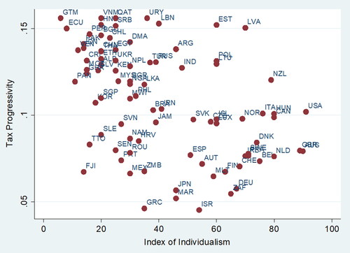
Figure 2. Pre-tax income inequality and tax progressivity.

Note: The values of Tax Progressivity and Individualism Index are averaged over the sample period between 1990 and 2005 for each of the 87 countries whose data are utilised for the regression analyses below. Each country is notated according to ISO 3-letter code.

Source: generated by this study.

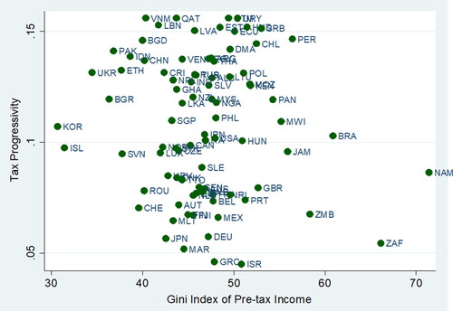
Table 1. Descriptive statistics.

Variable	Mean	(SD)
Tax Progressivity	0.064	(0.020)
Gini Index of Pre-tax Income	46.771	(6.488)
Index of Individualism	42.281	(23.276)
GDP Per Capita (PPP, 2011 international thousand dollars)	18.579	(16.473)
Total Population (million)	65.850	(184.012)
Population Share of Prime-Age Workers (%)	63.166	(5.788)
Involvement in Inter-State War (=1)	0.094	(0.293)
Parliamentary System (=1)	0.519	(0.500)
Legal Origin	Frequency	Share (%)
English Legal Origin	353	29.76
French Legal Origin	552	46.54
German Legal Origin	203	17.12
Scandinavian Legal Origin	78	6.58
OECD Member (=1)	0.370	(0.483)
EU Member (=1)	0.203	(0.402)
Number of Countries	87
Number of Observations	1186

(1) The variables with (=1) are binary indicators that take the value of one if the statement of the variable name is true and the value of zero otherwise.

Source: generated by this study.

Table 2. Effect of individualism on tax progressivity (random effect model).

Dependent Variable: Tax Progressivity	(1)	(2)	(3)	(4)	(5)
Pre-tax Income Inequality	0.0007 (0.0004)	0.0008* (0.0004)		0.0007 (0.0004)	0.0008* (0.0004)
Individualism		$-$0.0005*** (0.0001)	$-$0.0005*** (0.0001)		$-$0.0005*** (0.0001)
GDP per capita	$-$0.00003 (0.0001)	0.0001 (0.0001)	0.00015 (0.0001)	0.00002 (0.0001)	0.00015 (0.0001)
Total Population	$-$0.012 (0.011)	$-$0.012 (0.008)	$-$0.011 (0.007)	$-$0.012 (0.010)	$-$0.012 (0.007)
Population Share of Prime-Age Workers	0.0002 (0.0004)	0.0005 (0.0004)	0.0002 (0.0004)	0.0002 (0.0004)	0.0004 (0.0004)
Involvement in Inter-State War	$-$0.002 (0.003)	$-$0.002 (0.003)	$-$0.002 (0.003)	$-$0.002 (0.003)	$-$0.002 (0.003)
Parliamentary System			$-$0.003 (0.003)	$-$0.005 (0.003)	$-$0.002 (0.003)
Legal Origin			$-$0.001 (0.002)	$-$0.001 (0.002)	0.001 (0.002)
OECD member			0.005 (0.004)	0.002 (0.004)	0.005 (0.004)
EU member			$-$0.003 (0.002)	$-$0.004* (0.002)	$-$0.004* (0.002)
Year Indicators Included?	Yes	Yes	Yes	Yes	Yes
Number of Countries	87	87	87	87	87
Number of Observations	1186	1186	1186	1186	1186

(1) The notations of *, **, and *** refer to being statistically significant at 10%, 5% and 1% levels, respectively.

(2) In the parenthesis is standard errors that are robust to heteroscedasticity and clusters.

Source: generated by this study.

Table 3. Effect of individualism on tax progressivity (population average model).

Dependent Variable: Tax Progressivity	(1)	(2)	(3)	(4)	(5)
Pre-tax Income Inequality	0.001** (0.0005)	0.001* (0.0004)		0.001* (0.0005)	0.0008* (0.0004)
Individualism		$-$0.001*** (0.0001)	$-$0.0005*** (0.0001)		$-$0.0005*** (0.0001)
GDP per capita	0.0001 (0.0002)	0.00015 (0.0001)	0.00015 (0.0001)	0.0001 (0.0002)	0.00016 (0.00014)
Total Population	$-$0.030** (0.015)	$-$0.014 (0.009)	$-$0.010 (0.007)	$-$0.029** (0.014)	$-$0.015* (0.008)
Population Share of Prime-Age Workers	0.0004 (0.0004)	0.0005 (0.0004)	0.0002 (0.0004)	0.0004 (0.0005)	0.0004 (0.0004)
Involvement in Inter-State War	$-$0.002 (0.003)	$-$0.002 (0.003)	$-$0.002 (0.003)	$-$0.002 (0.003)	$-$0.002 (0.003)
Parliamentary System			$-$0.003 (0.003)	$-$0.003 (0.003)	$-$0.002 (0.002)
Legal Origin			$-$0.0009 (0.002)	$-$0.001 (0.002)	0.0006 (0.001)
OECD member			0.005 (0.004)	0.004 (0.004)	0.005 (0.004)
EU member			$-$0.003 (0.002)	$-$0.004* (0.002)	$-$0.0036 (0.002)
Year Indicators Included?	Yes	Yes	Yes	Yes	Yes
Number of Countries	87	87	87	87	87
Number of Observations	1186	1186	1186	1186	1186

(1) The notations of *, **, and *** refer to being statistically significant at 10%, 5% and 1% levels, respectively.

(2) In the parenthesis is standard errors that are robust to heteroscedasticity and clusters.

Source: generated by this study.

References

- Akerlof, G. (1997). Social distance and social decisions. Econometrica, 65(5), 1005–1027.
- Alm, J., & Torgler, B. (2006). Culture differences and tax morale in the United States and in Europe. Journal of Economic Psychology, 27(2), 224–246.
- Andrew Young School of Policy Studies. (2010). Andrew young school world tax indicators. International Studies Program.
- Andriani, L., Bruno, R., Douarin, E., & Stepien-Baig, P. (2022). Is tax morale culturally driven? Journal of Institutional Economics, 18(1), 67–84.
- Barro, R. (2000). Inequality and growth in a panel of countries. Journal of Economic Growth, 5(1), 5–32. (1): https://doi.org/10.1023/A:1009850119329
- Benabou, R. (2000). Unequal societies: Income distribution and the social contract. American Economic Review, 90(1), 96–129. https://doi.org/10.1257/aer.90.1.96
- Benabou, R. (2002). Tax and education policy in a heterogeneous‐agent economy: What levels of redistribution maximize growth and efficiency? Econometrica, 70(2), 481–517. https://doi.org/10.1111/1468-0262.00293
- Chetty, R. (2006). A new method of estimating risk aversion. American Economic Review, 96(5), 1821–1834. https://doi.org/10.1257/aer.96.5.1821
- Corneo, G. (2002). The efficient side of progressive income taxation. European Economic Review, 46(7), 1359–1368. https://doi.org/10.1016/S0014-2921(01)00162-3
- Diamond, P. (1998). Optimal income taxation: An example with a U-shaped pattern of optimal marginal tax rates. American Economic Review, 88(1), 83–95.
- Eugster, B., & Parchet, R. (2019). Culture and taxes. Journal of Political Economy, 127(1), 296–337. (1): https://doi.org/10.1086/700760
- Feldstein, M. (1969). The effects of taxation on risk taking. Journal of Political Economy, 77(5), 755–764. (5): https://doi.org/10.1086/259560
- Guerra, A., & Harrington, B. (2022). Regional variation in tax compliance and the role of culture. Economia Politica, 13, 1–14.
- Heathcote, J., Storesletten, K., & Violante, G. (2014). Consumption and labor supply with partial insurance: An analytical framework. American Economic Review, 104(7), 2075–2126. https://doi.org/10.1257/aer.104.7.2075
- Heathcote, J., Storesletten, K., & Violante, G. (2017). Optimal tax progressivity: An analytical framework. The Quarterly Journal of Economics, 132(4), 1693–1754. https://doi.org/10.1093/qje/qjx018
- Hofstede, G. (1980). Culture’s consequences: International differences in work-related values. Sage Publications.
- Hofstede, G., Hofstede, G. J., & Minkov, M. (2010). Cultures and organizations: Software of the mind. McGraw-Hill.
- Hubbard, A., Ahern, J., Fleischer, N., Van der Laan, M., Lippman, S., Jewell, N., Bruckner, T., & Satariano, W. (2010). To GEE or not to GEE: Comparing population average and mixed models for estimating the associations between neighborhood risk factors and health. Epidemiology, 21(4), 467–474. https://doi.org/10.1097/EDE.0b013e3181caeb90
- Ireland, N. (2001). Optimal income tax in the presence of status effects. Journal of Public Economics, 81(2), 193–212. https://doi.org/10.1016/S0047-2727(00)00108-0
- Kanbur, R., & Tuomala, M. (1994). Inherent inequality and the optimal graduation of marginal tax rates. The Scandinavian Journal of Economics, 96(2), 275–282. https://doi.org/10.2307/3440605
- Kimball, M., & Shapiro, M. (2008). Labor supply: Are the income and substitution effects both large or both small? NBER Working Paper No. 14208.
- Kornai, J., Mátyás, L., & Roland, G. (2008). Institutional change and economic behaviour. Palgrave MacMillan.
- La Porta, R., Lopez-de-Silanes, F., & Shleifer, A. (2008). The economic consequences of legal origins. Journal of Economic Literature, 46(2), 285–332. https://doi.org/10.1257/jel.46.2.285
- Ljungqvist, L., & Uhlig, H. (2000). Tax policy and aggregate demand management under catching up with the Joneses. American Economic Review, 90(3), 356–366. https://doi.org/10.1257/aer.90.3.356
- Lubrano, M. (2017). Lorenz curves, the Gini coefficient and parametric distributions. In Penn state lecture notes for the econometrics of inequality and poverty, https://citeseerx.ist.psu.edu/viewdoc/download?doi=10.1.1.642.7285&rep=rep1&type=pdf
- Ma, J., Raina, P., Beyene, J., & Thabane, L. (2013). Comparison of population-averaged and cluster-specific models for the analysis of cluster randomized trials with missing binary outcomes: A simulation study. BMC Medical Research Methodology, 13(1), 1–16. https://doi.org/10.1186/1471-2288-13-9
- Mankiw, G., Weinzierl, M., & Yagan, D. (2009). Optimal taxation in theory and practice. Journal of Economic Perspectives, 23(4), 147–174. https://doi.org/10.1257/jep.23.4.147
- Meltzer, A., & Richard, S. (1981). A rational theory of the size of government. Journal of Political Economy, 89(5), 914–927. https://doi.org/10.1086/261013
- Mirrlees, J. (1971). An exploration in the theory of optimum income taxation. The Review of Economic Studies, 38(2), 175–208. https://doi.org/10.2307/2296779
- Perotti, R. (1996). Growth, income distribution, and democracy: What the data say. Journal of Economic Growth, 1(2), 149–187. https://doi.org/10.1007/BF00138861
- Persson, M. (1995). Why are taxes so high in Egalitarian societies? The Scandinavian Journal of Economics, 97(4), 569–580. https://doi.org/10.2307/3440543
- Persson, T., & Tabellini, G. (1994). Is inequality harmful for growth? American Economic Review, 84(3), 600–621.
- Persson, T., & Tabellini, G. (2002). Political economics: Explaining economic policy. MIT Press.
- Peter, K. S., Buttrick, S., & Duncan, D. (2010). Global reform of personal income taxation, 1981–2005: Evidence from 189 countries. National Tax Journal, 63(3), 447–478. https://doi.org/10.17310/ntj.2010.3.03
- Slemrod, J., & Bakija, J. (2000). Does Growing Inequality Reduce Tax Progressivity? Should It? NBER Working Paper 7576.
- Solt, F. (2016). The standardized world income inequality database. Social Science Quarterly, 97(5), 1267–1281. https://doi.org/10.1111/ssqu.12295
- Tsakumis, G., Curatola, A., & Porcano, T. (2007). The relation between national cultural dimensions and tax evasion. Journal of International Accounting, Auditing and Taxation, 16(2), 131–147. https://doi.org/10.1016/j.intaccaudtax.2007.06.004
- Werning, I. (2007). Optimal fiscal policy with redistribution. The Quarterly Journal of Economics, 122(3), 925–967. https://doi.org/10.1162/qjec.122.3.925
- Wynter, C. B., & Oats, L. (2018). Don’t worry, we are not after you! Anancy culture and tax enforcement in Jamaica. Critical Perspectives on Accounting, 57, 56–69. https://doi.org/10.1016/j.cpa.2018.01.004
- Yong, S., & Martin, F. (2016). Tax compliance and cultural values: The impact of individualism and collectivism on the behaviour of New Zealand small business owners. Australian Tax Forum, 31, 289–320.