Development of an income and cost simulation model for studio apartment using probabilistic estimation

ABSTRACT

The Korean construction industry has attracted interest and investment demand for lease-oriented investment products, such as shopping malls and studio apartments, as a substitute for financial products because of the low interest rates of the banks that resulted from the economic recession after the global financial crisis in 2008. However, there have been huge economic damages because of problems such as the oversupply, the increase in the unsold presale rate, and the decrease in rental profit. For studio-apartment development projects, dynamic analysis should be applied considering the correlation of variables in business analysis, which is complicated by such factors as profit structure and money flow. Therefore, we aim in this study to develop a statistical analysis model of studio apartments using probabilistic estimation. For this purpose, we developed a causal-loop diagram and established a simulation and optimization model. The developed model was verified by applying it to actual cases. Our results can be used as a reference for the optimization and risk management of studio-apartment business analysis in academia. In addition, from a practical point of view, this model can be used to develop a forecasting feasibility study based on risk and for business feasibility analysis.

Graphical Abstract

KEYWORDS:

• Studio apartment
• probabilistic estimation
• system dynamics
• risk analysis

1. Introduction

The Korean construction industry has had increased interest and investment in lease-based investment products, such as shopping malls and studio apartments, as a substitute for financial products because of the low interest rates of banks that resulted from the economic downturn after the global financial crisis in 2008 (Cho 2015). In particular, studio apartments are free from regulations, such as strengthening loan screening and resale that are applied to larger apartments, and leasing demand is also relatively high because of the rapid increase in one-person households (Jang et al. 2018). As a result, the supply of new studio apartments has steadily increased since 2010, exceeding the first 30,000 in 2011, 48,000 in 2014, and the highest in 2017 at 68,233 (Jang et al. 2019).

However, according to Real Estate 114, Korea’s largest provider of real-estate information, 31,943 rooms (46%) out of the total 68,823 office buildings sold nationwide in 2017 were not sold until early March 2018. Studio apartments’ rental yield has also been declining. It declined to 6.01% in 2011, 5.95% in 2012, 5.87% in 2013, 5.81% in 2014, 5.70% in 2015, 5.45% in 2016, and 5.22% in 2017, and plunged to 0.59% (Ministry of Land, Infrastructure and Transport, Republic of Korea).

This decline in rental yields has had a negative effect on the studio-apartment supply, which has increased until recently, and has caused massive damage to society, including the bankruptcy of large-scale construction companies and economic damage to persons who had been given a studio apartment.

For example, the continuous decline of studio apartments is related to decrease occupancy rate as well as new project promotion. In this respect, these can be caused severe financial stress to the construction companies and ultimately decrease of housing supply. Especially, since current occupancy rate of presold studio apartment is low, the private construction companies suffered from the difficulty of balance recovery by increased default rate. Therefore, accurately predicting business risks early in development is critical to the success of the project (Isaac and Navon 2009).

Park and Choi (Park and Choi 2013) carried out a feasibility analysis of existing studio-apartment development projects by means of deterministic analysis, which relies on one representative value. However, it can be considerably changed between initial plan and final result since it takes a long time for the land development (Yu et al. 2017). In this respect, the deterministic method is difficult to analyze the impact of influential factors quantitatively (Zavadskas, Turskis, and Tamošaitiene 2010).

In addition, for successful project, the developer should decide whether or not the project progress by predicting cash flow of investment cost and establishing the control range of influential factors. In this respect, the profit is directly related to manage the range of the factors such as land costs, construction costs, sales price, financial costs. If the factors can be simulated with actual price of surrounding area, the control range of these factors can be identified then the developer can predict various project costs effectively by simulating influential factors.

Therefore, for studio-apartment development projects, dynamic analysis is required because it has a complex system dealing with, e.g., profit structure and flow of funds. In particular, among the probabilistic analysis methods, the system dynamics technique can analyze the dynamic relationship between influential factors and make a dynamic analysis according to the change of variables (Park et al. 2008; Son 2007; Sin 2012; Park 2018; Son 2018). In this respect, the objective of this study is to develop a financial analysis model for studio apartments using stochastic estimation such system dynamics technique.

The findings of this study suggest that it is possible to create a forecasting feasibility study of risk based on the practical application of studio apartments, which provides a basis for optimizing the risk management of studio apartments.

2. Methodology

The methodology of this study is as shown in Figure 1. First, the risk factors directly affecting profits on the studio apartment development project are examined and the methodologies such as system dynamics and Monte Carlo simulation are investigated.

Figure 1. Methodology

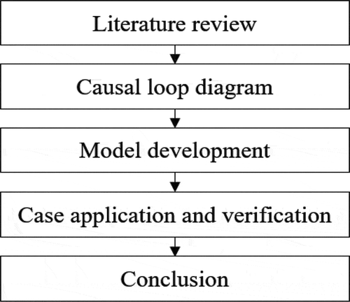
Second, the casual loop diagrams are created by analyzing causal relationships among the major risk factors defined above. Third, based on the created casual loop diagram, an income and cost simulation and an optimization model sequentially are constructed. Then, the Monte Carlo simulation is used to set the control limits for each factor. Finally, the simulation results are obtained through this support the decision-making of the owner in the studio-apartment development project.

3. Literature reviews

3.1. Analysis of factors that influence risk

There have been many studies on the factors affecting the building development business. However, most studies have shown that factors influencing the success or failure of a business are macro level factors, such as changes in political environment and government policy (Rachmawati et al. 2018; Shi Ming and Chee Hian 2005) and changes in market demand (Caldera and Johansson 2013; Michael, Vicky, and Michael 2002), and project-level factors, such as market level (Go et al. 2005) and appropriateness of business method and fundraising ability (Ferreira and Jalali 2015; Koo and Jung 2007), and listed only the effect of factors on business performance (Rachmawati et al. 2018; Shi Ming and Chee Hian 2005; Michael, Vicky, and Michael 2002; Go et al. 2005; Koo and Jung 2007). In other words, they failed to quantitatively and clearly calculate the relationship between these qualitative factors and profit as a business performance. Therefore, it is very difficult to use them for practical purposes. In order to solve this problem, we developed a model which is limited to factors that have a more direct effect on the profit of the project. As shown in Table 1, there are six main influencing factors (Jang et al. 2019; Sin 2012; Park 2018; Son 2018; El-Sayegh and Mansour 2015; Lee 2017).

Table 1. Previous studies about influence factors

Author	Risk influence factors
	Period	Sales ratio	Sales price	Building costs	Land costs	Finance costs
Jang (2019)		●	●			●
Sin (2012)	●	●	●	●	●	●
Park (2018)		●	●	●	●	●
Son (2018)	●	●	●	●	●	●
Sayegh (2015)				●	●	●
Lee (2017)	●	●	●	●	●	●

In terms of risk management, the qualitative factors mentioned above are reflected in the surrounding market prices, the nearby land prices, and the nearby prevalence rate, and as a result, they are expressed as sales price, land cost, construction cost, sales ratio, and so on (Sin 2012; Park 2018; Son 2018; Lee 2017). These studies are limited to the key factors that directly affect the project profit and define the variables used in the overall profitability and risk analysis of the project. Therefore, we consider s seven factors, which are direct selling price, presale rate, presale period, construction cost, land cost, and financial cost.

3.2. System dynamics

System dynamics is based on a causal-loop diagram (Sterman 2001), which is a structural reflection of the problems as shown in Table 2.

Table 2. Comparison between existing deterministic analysis and system dynamics methodology (Son 2007, 2018; Sterman 2001)

Characteristics	Traditional deterministic analysis	System dynamics
Object of analysis	Static form (point estimation)	Dynamic form type
(2)Inference method	Causal relationship of existing empirical data	Causal relationship of variables
(3)Analysis focus	The relationship between two variables	Circular relations between variables
(4)Goal of analysis	Pursuit of numerical accuracy	Pursuing structural accuracy
(5)Object of knowledge	Observable objective phenomena	Feedback structure
(6)Definitions of Understanding	Difficulty (numerical expression)	Easy (using graphs and diagrams)

Based on the causal-loop diagram, it is possible that forecast how a specific variable changes dynamically over time (Son 2007). In other words, unlike the existing deterministic method of deriving an estimated value of an event or a variable, system dynamics can identify the dynamic change of the variable over time (Son 2018). Therefore, we intend to develop a causal model for the analysis of the major balance-sheet items affecting studio-apartment development projects, and to develop a balance-sheet analysis model based on this

3.3. Monte Carlo simulation

Monte Carlo simulation is a probabilistic analysis method used to obtain the solution of the input variable by means of a probability model and random numbers (Lee 2017). The Monte Carlo technique allows precise simulation, because the distribution of input values is constant. In addition, for applying a probability distribution suitable for a given problem, an algorithm for generating a random number following the probability distribution is important (Jeon 2015). Therefore, Monte Carlo simulation can be used to study the prediction of the appropriate time and cost range considering the effects of risk (Lee 2017; Jeon 2015; Peleskei et al. 2015). We construct a range of variance and an optimization model based on major uncertainties arising from studio-apartment business balance analysis through Monte Carlo simulation.

4. Model development

The developed model in this study is divided into t₀-t₃ as shown in Figure 2. The t₀ proceeds the economic feasibility analysis of the project as the initial project review. In the t₀, if the feasibility is confirmed by the simulation model, the target land is purchased. The t₁ is the acquisition process regarding building permit. In this phase, the project contents such as the number of buildings, housing units, building heights, building coverage and volume can be changed unlike initial planning. As a result, the sales price should be reviewed again by the suggested simulation model in this phase since profit can be changed.

Figure 2. Simulation phases

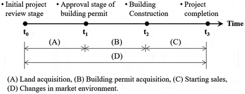
The t₂ is the phase of building construction and starting sales at the same time. The final sales price has to be decided in this phase after simulating the sales price by suggested model. If the feasibility is not good, the developer can be made decisions such as the return rate change and taking risks.

Therefore, the objective of the suggested model is to manage the profit by using stochastic method such dynamic simulation. The model can set the control range regarding influence factors and support the decision of the developer from the results of simulation model.

4.1. Casual-loop diagram

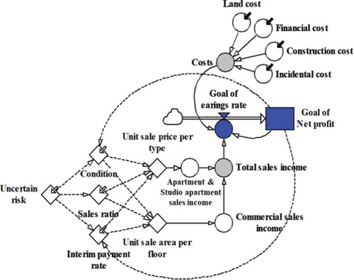
Using the system dynamics method, we analyzed the causal relationship based on the factors selected in Table 1. The causal-loop diagram of risk factors is shown in Figure 3.

Figure 3. Causal-loop diagram

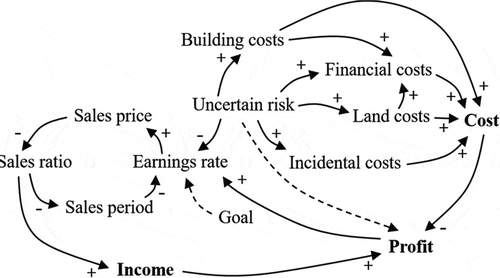
To explain the causal relationship in Figure 3, the business success of the studio-apartment development project is determined by the profit of the project. Business profits are determined by the level of income (income) and expenditure (cost). At this time, the level of income is determined by the sales price and the sales ratio, and the expenditure is determined by the level of building costs, land costs, and financial costs (Choi et al. 2017).

For income, there is a negative correlation with the subsequent variables in the process leading to the presale rate and presale income. This structure should adjust the selling price by adjusting the target rate of return when the presale rate is low and profit is decreased. Decreasing presale prices will increase the willingness of potential buyers to buy, which may lead to an increase in the presale rate, which means an increase in total presale revenue. For expenditure, there is a positive correlation with construction cost, land cost, and finance cost. In addition, since the construction cost and the land cost are expenditures in the financial cost, the two variables and the financial cost have a positive (+) relationship. In particular, if uncertain risks such as land costs and lending rates rise, land and finance costs will increase and the total business costs will increase. Increased business costs are directly linked to business profits, forming a feedback loop. In this way, it is the range of the various influencing factors (variables) related to these that determine the change in sales revenue or business expense. Therefore, we used the probabilistic estimation technique to simulate presale income and business expenditure within the range of influence variables and to confirm the business profit.

4.2. Income and cost simulation model

4.2.1. Income simulation model

The income simulation model consists of variables, such as sales income, sales ratio, and interim payment schedule, as shown in Figure 4.

Figure 4. Income simulation model

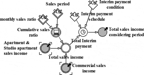
The import model in Figure 4 is described in more detail. First, the monthly sales ratio, the interim payment condition, and the interim payment condition are input. The total sales income is then calculated by automatically calculating the cumulative sales ratio, apartment and studio-apartment sales income, and commercial sales income, which reflects the ainterim payment schedule and the interim payment condition in the calculated total sale revenue. As a result, we can identify the structure of cash flows for income over time.

At this time, the apartment sales, studio-apartment sales, and commercial

sales income are modeled automatically, as shown in Figure 5. In Figure 5(a), the apartment and studio-apartment sales model is designed so that it can input equilibrium ($A_i$), household number ($N_i$), and unit sale price ($P_i$) for each type. Then, the total presale income of apartments and studio apartments is automatically calculated through Equation (1)(1) $I_s=\sum _i^l{P}_i\times N_i\times A_i$(1) . The calculated results are interrelated with the income simulation model in Figure 4.

(1) $I_s=\sum _i^l{P}_i\times N_i\times A_i$(1)

Figure 5. Sales income model

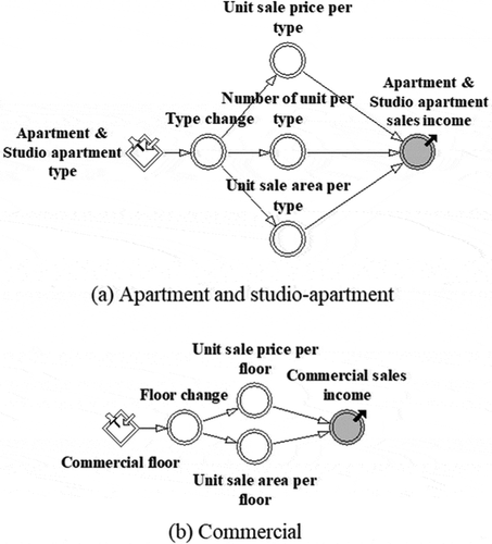
Here, $I_s$: apartment and studio-apartment sales income, $P_i$: unit sale price, $N_i$: the number of units, $A_i$: the sale area of each unit, i: the number of unit types.

Figure 5(b) shows the number of floors (j), balances ($A_j$), and units sold ($P_j$). Then, the total sales revenue of the shopping mall is automatically calculated through Equation (2)(2) $I_c=\sum _j^m{P}_j\times A_j$(2) . The calculated results are connected with the import simulation model in Figure 4.

(2) $I_c=\sum _j^m{P}_j\times A_j$(2)

Here, $I_c$: commercial sales income, $P_j$: the sales price per m² in each floor, $A_j$ sale area of each floor, j: the number of floors.

4.2.2. Cost simulation model

The cost simulation model of this study consists of financial costs, land costs, construction costs, and incidental costs, as shown in Figures 6 and 7. The core of these is the financial costs model in Figure 6, because, if the initial presale rate increases after the start of the sale, no trouble will arise if it is possible to obtain a smooth fund (Huh, Hwang, and Lee 2012). In other words, it is possible to increase the profits by repaying the initial costs for project finance and other financial costs. However, if not, it is difficult to predict the circulation of funds. A major cause of business failure is their not being able to redeem the financial expenses (Warszawski 2003). Most of the recent real-estate development business failures can be found in financial cost forecast failure (Lee, Lee, and Kim 2016; Warszawski 2003). Therefore, we constructed the simulation model by linking the financial cost generated during the project promotion with the import model.

Figure 6. Financial cost model

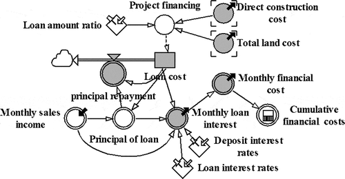
The financial cost model in Figure 6 consists of project financing cost ($F_{proj}$), loan amount ratio ($A_{loan}$), principal of loan ($L_{prin}$), and interest on loans ($I_{loan}$). The project financing cost ($F_{proj}$) is calculated as the product of land purchase cost ($C_{land}$), direct construction cost ($C_{dire}$), and loan interest rate ($R_{loan}$), as shown in Equation (3)(3) $F_{proj}=\left(C_{land}+C_{dire}\right)\times R_{loan}$(3) . The ratio of the loan ($A_{loan}$) can be obtained by subtracting the capital ratio ($R_{capi}$) from 1, as shown in Equation (4)(4) $A_{loan}=1-R_{capi}\times 100$(4) . Also, the project financing cost ($F_{proj}$) is a component of the subsequent variable, loan cost ($C_{loan}$), and the loan amount ($C_{loan}$) is a component of the principal repayment amount ($L_{prin}$). At this time, the principal repayment amount ($L_{prin}$) is found by comparing it with monthly sales income ($S_{mont}$), as shown in Equation (5)(5) $L_{prin}=if(C_{loan}<S_{mont},C_{loan},S_{mont})$(5) . The loan interest rate ($R_{loan}$) is applied to the period during which the project financing cost ($F_{proj}$) is repaid, as shown in Equation (6)(6) $I_{loan}=if\left(C_{loan}>L_{prin},C_{loan}\times R_{loan},S_{mont}\times R_{depo}\right)$(6) , and the deposit interest rate ($R_{depo}$) is applied to the sale income after the principal repayment is completed. Consequently, the financial-cost model of this study can estimate the financial cost over time by automatically calculating the principal repayment amount according to the presale income level.

(3) $F_{proj}=\left(C_{land}+C_{dire}\right)\times R_{loan}$(3)

(4) $A_{loan}=1-R_{capi}\times 100$(4)

(5) $L_{prin}=if(C_{loan}<S_{mont},C_{loan},S_{mont})$(5)

(6) $I_{loan}=if\left(C_{loan}>L_{prin},C_{loan}\times R_{loan},S_{mont}\times R_{depo}\right)$(6)

Here, $F_{proj}$: financial cost, $C_{land}$: land cost, $C_{dire}$: direct construction cost, $R_{loan}$: loan interest rate, $A_{loan}$: loan amount ratio, $R_{capi}$: capital ratio, $L_{prin}$: principal repayment amount, $C_{loan}$: loan cost, $S_{mont}$: monthly sales income, $I_{loan}$: loan interest.

The land cost, construction cost, and incidental cost models are shown in Figure 7. The land cost in Figure 7(a) is calculated by multiplying the land cost for each lot by the land area for each lot and the other land acquisition costs.

Figure 7. Land, construction, and incidental cost model

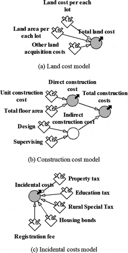
The construction cost in Figure 7(b) is calculated as the sum of direct construction cost and indirect construction cost. Direct construction costs consist of unit construction cost and total floor area. Indirect construction costs include design and supervising. The incidental costs of Figure 7(c) include property tax, education tax, rural special tax, housing bonds, and registration fees.

5. Profit simulation model

As seen in Figure 8, the optimization model of this study can feed back the presale revenue and business costs by uncertain risks.

Figure 8. Income and cost optimization model

In addition, this model can set a control limit for each factor to achieve the target return. The business entity can manage the business so as not to escape. Moreover, the business entity can select an optimal solution that is suitable for the situation and conditions among the alternatives through the simulation. In this case, the formula for calculating profit, income, and cost of the analytical model is Equations (7)(7) $Profit=\sum _k^m\left(Incom{e}_k-Cos{t}_k\right)\pm U{r}_k$(7) , (8(8) $Incom{e}_k=\sum _k^m\left(I_s+I_c\right)\times C_{interim}\times R_{interim}\pm U{r}_k$(8) ), (9(9) $Cos{t}_k=\sum _k^m\left(C_{land}+C_{cons}+C_{inde}+F_{proj}\right)\pm U{r}_k$(9) ). In order to simulate changes in funding over time, the number of months (k) from the start of the project to the end of the project is set as a variable.

(7) $Profit=\sum _k^m\left(Incom{e}_k-Cos{t}_k\right)\pm U{r}_k$(7)

(8) $Incom{e}_k=\sum _k^m\left(I_s+I_c\right)\times C_{interim}\times R_{interim}\pm U{r}_k$(8)

(9) $Cos{t}_k=\sum _k^m\left(C_{land}+C_{cons}+C_{inde}+F_{proj}\right)\pm U{r}_k$(9)

Here, $Incom{e}_k$: monthly sales income, $Cos{t}_k$: monthly project cost, $I_s$: apartment and studio-apartment sales income, $I_c$: commercial sales income, $C_{interim}$: intermediate payment schedule, $R_{interim}$: intermediate payment rate, $C_{land}$: land cost, $C_{cons}$: construction costs,$C_{inci}$: incidental costs, $F_{proj}$: financial costs, $U{r}_k$: uncertain risks, k: the number of months from project commencement to completion

As shown in Equation (7)(7) $Profit=\sum _k^m\left(Incom{e}_k-Cos{t}_k\right)\pm U{r}_k$(7) , profit is calculated as the difference between total business costs and income. The income of Equation (7)(7) $Profit=\sum _k^m\left(Incom{e}_k-Cos{t}_k\right)\pm U{r}_k$(7) is calculated as the sum of the sales income of each item (i.e., studio apartment, apartment, and shop), as shown in Equation (8)(8) $Incom{e}_k=\sum _k^m\left(I_s+I_c\right)\times C_{interim}\times R_{interim}\pm U{r}_k$(8) . At this time, the flow of funds is determined by the intermediate payment schedule ($C_{interim}$) and the intermediate payment rate ($R_{interim}$), and is changed by uncertain risks ($U{r}_k$) such as low presale rate, schedule change of intermediate payment rate, and ratio. In addition, the total project cost can be calculated as the sum of land costs ($C_{land}$), construction costs ($C_{cons}$), incidental costs ($C_{inci}$), and financial costs ($F_{proj}$), as shown in Equation (9)(9) $Cos{t}_k=\sum _k^m\left(C_{land}+C_{cons}+C_{inde}+F_{proj}\right)\pm U{r}_k$(9) . However, it is subject to uncertain risks ($U{r}_k$), such as land expense exceeding the projected amount, or excessive financial costs.

6. Case study

The case study is conducted in this section for the validation of the developed model. The model can be applied in each phase from t₀ to t₃. The developer sets the risk management limit regarding influential factors such as presale price, sale period, land cost, construction cost, finance cost, and other expenses to achieve the target profit. If the planned sales ratio is appropriate before t₃ phase, the target profit can be achieved. However, the sales ratio is not fit, the sales price can be changed by conducting the simulation of income and cost.

Table 3 shows the overview of a case project. The project consists of 298 households, 430 studio apartment, shopping malls of 28,050 m². The land was purchased by 1,460 USD/m² in the case project and households, studio apartment and shopping mall were sold by 3,291 USD/m², 2,278 USD/m², and 5,063 USD/m² respectively. The project was predictable that it is sold out within 6 months after selling starts. However, the return rate (10.3%) could not be achieved by low sales ratio.

Table 3. Overview of a case project

Description	Contents
Project title	DWC studio apartment development
Location	Goyang, Gyeonggi, Korea
Site area	12,919 m^2
Total floor are	172,240 m^2
Building area	6,699 m^2
Number of units	Apartment: 298 units (2 types) Studio apartment: 430 units (2 types) Shopping mall: 28,050 m^2 (area supplied)
Construction period	28 months

The conventional deterministic feasibility analysis cannot be predictable the dynamic variation due to the change of sales ratio and interests. In other words, it is difficult to response risks before identifying the results of the project. However, in the developed model, the profit can be predictable by simulating the influential factors according to the cash flow

6.1. Initial review phase

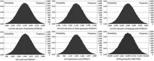
Table 4 shows the initial input value of influential factors in the initial project review stage. These values were applied in the developed model and 100,000 random numbers that follows the lognormal distribution were generated. These values were used to decide the range of the profit variation.

Table 4. Initial input values

Item	Unit	Initial value
Unit sale price 1. Apartment 2. Studio apartment 3. Shopping mall	USD/m^2	3,291 2,278 5,063
Land cost	USD/m^2	1,460
Construction cost	USD/m^2	1,316
Incidental cost	USD/m^2	222
Loan interest rates	%	4.3
Deposit interest rates	%	2.7
Project period	Months	28

KRW 1,197.00 = USD 1.00 as of 2019/10/06 (Bank of Korea)

As a result, as shown in Table 5 and Figure 9, the average of apartment was 3,291 USD/m², the maximum was 4,607 USD/m², the minimum was 1,810 USD/m². The average of studio apartment and shopping mall was 2,278 USD/m², and 5,063 USD/m², respectively. In addition, the average of land cost was 1,460 USD/m², the maximum was 2,044 USD/m², the minimum was 803 USD/m² and the average of construction cost was 1,316 USD/m². Finally, due to the variation of these influence factors, the profit variation was identified from −49,477,000 USD to 120,153,000 USD.

Table 5. Result of simulation

Item	Average	Maximum	Minimum
Unit sale price (USD/m^2) 1. Apartment 2. Studio apartment 3. Shopping mall	3,291 2,278 5,063	4,607 3,189 7,088	1,810 1,253 2,785
Land cost (USD/m^2)	1,460	2,044	803
Construction cost (USD/m^2)	1,316	1,842	724
Profit (1,000 USD)	34,042	120,153	−49,477

KRW 1,197.00 = USD 1.00 as of 2019/10/06 (Bank of Korea).

Figure 9. Random variable generation

As shown in Table 6, if the target return rate by the developer sets from 10% to 12%, the sales prices of apartment, studio apartment and shopping mall should be decided to the range such as 2,534–3077 USD/m³, 1,754–2,130 USD/m³, and 3,899–4,734 USD/m³ respectively. In addition, land cost and construction cost have to decide in the range such as 924–1,128 USD/m³, and 842–1,027 USD/m³. If the profit is out of the control limit, the new plan such the change of return rate should be established.

Table 6. Setting the control limit of risk factors

		Unit sale price (USD/m^2)
No. of trials	Earnings rate (%)	Apartment	Studio apartment	Shopping mall	Land cost (USD/m^2)	Construction cost (USD/m^2)
1	−29.70	1,810	1,253	2,785	2,044	1,842
2	−29.69	1,932	1,260	2,793	2,003	1,820
…	…	…	…	…	…	…
52,101	10.02	2,534	1,754	3,899	1,128	1,027
52,102	10.04	2,541	1,762	3,891	1,124	1,013
…	…	…	…	…	…	…
99,999	39.68	4,600	2,992	6,998	868	759
100,000	39.69	4,607	3,189	7,088	803	724

KRW 1,197.00 = USD 1.00 as of 2019/10/06 (Bank of Korea).

Therefore, the developed model can be predictable the return rate according to the change of influential factors. In addition, the upper and lower range limit can set by conducting simulation. In this respect, the developer can achieve the target profit if the factors can manage within the limit.

6.2. Review phase after identifying low sales ratio

If there is lower sale ratio than initial plan, the developer should make a decision regarding project progress. In the t₂ phase, the land cost and construction cost were determined. In this case, the key factors are residual sales ratio and financial cost.

For example, as shown in Table 3, the sales ratio of the case project was 20% (10%, 6%, and 4%) in early 3 months. This result is one-third level of the predicted rate of t₀(60%). Accordingly, the financial cost will be increased because of low sales ratio. As a result, it was failed to achieve the target return rate. In this respect, this study conducted the simulation the financial cost and the profit using the assumption deducting rate by 5% in the original sales price. The simulation result represents Figure 10 and Table 7.

Figure 10. Simulation results of financial cost and profit

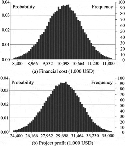
Table 7. Simulation results of financial cost and profit for changes in residual sales ratio

Unit: 1,000 USD
No. of trials	M + 3	M + 4	M + 5	M + 6	…	M + 11	M + 12	Total	Financial cost	Profit
1	12%	11%	10%	10%	…	3%	2%	100%	11,884	24,375
2	12%	10%	11%	8%	…	5%	5%	100%	10,456	25,287
…	…	…	…	…	…	…	…	…	…	…
999	24%	18%	17%	16%	…	0%	0%	100%	8,415	34,983
1000	25%	23%	17%	15%	…	0%	0%	100%	8,398	35,063

As shown in Table 7, the simulation repeated by 1,000 and average financial cost was 9,993,000 USD, maximum and minimum were 11,884,000 USD and 8,398,000 USD. In addition, the average profit was 30,783,000 USD, maximum and minimum were 35,063,000 USD and 24,375,000 USD. Therefore, to achieve the maximum profit, the developer has to sell them within 4 months. If the planned rate could not be achieved in next month, the developer should establish new plan by using the model. In this method, according to time flow, the developed model can be repeated.

7. Conclusion

In this study, the income and cost simulation, and profit model of studio-apartment development projects was developed. This allows a developer to control sales income and business costs within the range of variables that affect cost and income, so that the profits remain positive. In addition, the developed model proved its effectiveness through case study.

As a result, first, the simulation model can predict the range limit of influential factors by analyzing the causal loop diagram between project costs (financial costs, construction costs, land costs, and other costs) and factors influencing earnings (presale prices, presale period, presale rate). In the case project, the simulation result shows that the average of profit was 34,042,000 USD, maximum and minimum were 120,153,000 USD and 49,477,000 USD.

Second, it is possible to derive the management scope for each factor to achieve the target return rate by using simulation results. For the case project, if the target rate of return is 10% ~ 12%, the sales price of apartments, studio apartments, and shopping malls should be managed within 2,534–3,077 USD/m², 1,754 ~ 2,130 USD/m², and 3,899 ~ 4,734 USD/m², respectively.

Third, the developed model can support the developer’s decision when there is low sales ratio in early phase. For the case project, if the 5% deductible sales price is applied when the appropriate sales ratio cannot be achieved within 3 months after starting sales, the predicted profit can be changed from 24,375,000 USD to 35,063,000 USD.

Therefore, the developed model can be predictable the influential factors and conducted simulation results in advance. The findings of this study can be utilized the fundamental materials for developing optimization and risk management model to reduce economic losses in studio apartment project.

Disclosure statement

No potential conflict of interest was reported by the authors.

Additional information

Funding

This research was funded by Basic Science Research Program through the National Research Foundation of Korea (NRF) funded by the Ministry of Education (NRF-2019R1F1A1058800).

References

- Caldera, A., and Å. Johansson. 2013. “The Price Responsiveness of Housing Supply in OECD Countries.” Journal of Housing Economics 22 (3): 231–249. doi:https://doi.org/10.1016/j.jhe.2013.05.002.
- Cho, Y. C. 2015. “A Study on the Decision Making of Officetel Development Project.” PhD diss., Jeon-Ju University, Republic of Korea.
- Choi, M., M. Park, H. S. Lee, and S. Hwang. 2017. “Dynamic Modeling for Apartment Brand Management in the Housing Market.” International Journal of Strategic Property Management 21 (4): 357–370. doi:https://doi.org/10.3846/1648715X.2017.1315347.
- El-Sayegh, S. M., and M. H. Mansour. 2015. “Risk Assessment and Allocation in Highway Construction Projects in the UAE.” Journal of Management in Engineering 31 (6): 04015004-1-10. doi:https://doi.org/10.1061/(ASCE)ME.1943-5479.0000365.
- Ferreira, F. A., and M. S. Jalali. 2015. “Identifying Key Determinants of Housing Sales and Time-on-the-market (TOM) Using Fuzzy Cognitive Mapping.” International Journal of Strategic Property Management 19 (3): 235–244. doi:https://doi.org/10.3846/1648715X.2015.1052587.
- Go, S. S., J. H. Hong, H. Song, and H. K. Park. 2005. “A Study on the Trend of Apartment Brand and the Residents’ Preference.” Architectural Institute of Korea 25 (1): 19–22.
- Huh, Y. K., B. G. Hwang, and J. S. Lee. 2012. “Feasibility Analysis Model for Developer-proposed Housing Projects in the Republic of Korea.” Journal of Civil Engineering and Management 18 (3): 345–355. doi:https://doi.org/10.3846/13923730.2012.698911.
- Isaac, S., and R. Navon. 2009. “Modeling Building Projects as a Basis for Change Control.” Automation in Construction 18 (5): 656–664. doi:https://doi.org/10.1016/j.autcon.2009.01.001.
- Jang, J. H., S. G. Ha, K. R. Kim, K. Y. Son, S. H. Son, and T. O. Lee. 2018. “Feasibility Model Development by Applying System Dynamics Method in Residential Officetel.” Journal of the Korea Institute of Building Construction 18 (3): 285–294. doi:https://doi.org/10.5345/JKIBC.2018.18.3.285.
- Jang, J. H., S. G. Ha, K. Y. Son, and S. H. Son. 2019. “Financial Analysis Model Development by Applying Optimization Method in Residential Officetel.” Journal of the Korea Institute of Building Construction 19 (1): 67–76. doi:https://doi.org/10.5345/JKIBC.2019.19.1.067.
- Jeon, J. M. 2015. “A Study on the Price Determinants of Officetel: Focusing in Youngdeungpo-gu.” Masters diss., Yeonsei University, Republic of Korea.
- Koo, S. M., and M. W. Jung. 2007. “A Basic Study on the Current State and Problems of Feasibility Study-focused on the Evaluation Criteria of the Existing Relative Researches.” Architectural Institute of Korea 23 (9): 79–88.
- Lee, G. S. 2017. “An Study on Analysis of Risk Factor for Developing Officetel.” Masters diss., Hanyang University, Republic of Korea.
- Lee, Y. H., S. H. Lee, and J. J. Kim. 2016. “Development of the Housing Business Model to Minimize the Fluctuation Risk of the Housing Market.” Journal of the Korea Academia-Industrial Cooperation Society 17 (10): 635–646. doi:https://doi.org/10.5762/KAIS.2016.17.10.635.
- Michael, B., S. Vicky, and S. Michael. 2002. “Residential Real Estate Prices: A Room with a View.” Journal of Real Estate Research 23 (1–2): 129–138. doi:https://doi.org/10.5555/rees.23.1-2.m2252681kl24h0th.
- “Ministry of Land, Infrastructure and Transport, Republic of Korea.” http://rt.molit.go.kr/
- Park, J. B., Y. Cho, K. B. Kwon, and J. H. Paek. 2008. “Feasibility Analysis Model Study of Realestate Development - Focused on Construction Project Development of Apartment and Stores.” Journal of Architectural Institute of Korea 24 (3): 179–186.
- Park, J. Y. 2018. “A System Development for Risk Management of Apartment Building Projects Using System Dynamics.” PhD diss., Kyung Hee University, Republic of Korea.
- Park, K. Y., and S. D. Choi. 2013. “Analysis of Key Influential Variables and Their Impacts on Hotel Development Project Financial Feasibility Analysis Using Stochastic System Dynamics Method.” International Journal of Tourism Sciences 37 (9): 317–337.
- Peleskei, C. A., V. Dorca, R. A. Munteanu, and R. Munteanu. 2015. “Risk Consideration and Cost Estimation in Construction Projects Using Monte Carlo Simulation.” Management (18544223) 10 (2): 163–176.
- Rachmawati, F., R. A. A. Soemitro, T. J. W. Adi, and C. Susilawati. 2018. “Critical Success Factor for Partnership in Low-cost Apartments Project: Indonesia Perspective.” Pacific Rim Property Research Journal 1–12. doi:https://doi.org/10.1080/14445921.2018.1461769.
- Shi Ming, Y., and C. Chee Hian. 2005. “Obstruction of View and Its Impact on Residential Apartment Prices.” Pacific Rim Property Research Journal 11 (3): 299–315. doi:https://doi.org/10.1080/14445921.2005.11104189.
- Sin, D. H. 2012. “A Risk Analysis Model for Apartment Building Project.” PhD diss., Kyung Hee University, Republic of Korea.
- Son, K. Y. 2007. “A Model for Feasibility Analysis of Commercial Buildings.” Masters diss., Kyung Hee University, Republic of Korea.
- Son, S. H. 2018. “A Simulation Model for Feasibility Analysis of Apartment Building Projects Using System Dynamics” Masters diss., Kyung Hee University, Republic of Korea.
- Sterman, J. D. 2001. “System Dynamics Modeling: Tools for Learning in a Complex World.” California Management Review 43 (4): 8–25. doi:https://doi.org/10.2307/41166098.
- Warszawski, A. 2003. “Parametric Analysis of the Financing Cost in a Building Project.” Construction Management and Economics 21 (5): 447–459. doi:https://doi.org/10.1080/0144619032000049638.
- Yu, Y. J., K. Y. Son, T. H. Kim, and J. M. Kim. 2017. “A Risk Quantification Study for Accident Causes on Building Construction Site by Applying Probabilistic Forecast Concept.” Journal of the Korea Institute of Building Construction 17 (3): 287–294. doi:https://doi.org/10.5345/JKIBC.2017.17.3.287.
- Zavadskas, E. K., Z. Turskis, and J. Tamošaitiene. 2010. “Risk Assessment of Construction Projects.” Journal of Civil Engineering and Management 16 (1): 33–46. doi:https://doi.org/10.3846/jcem.2010.03.