AI-based Lagrange optimization for designing reinforced concrete columns

ABSTRACT

Structural engineers face several code-restricted design decisions. Codes impose many conditions and requirements to the designs of structural frames, such as columns and beams. However, it is difficult to intuitively find optimized solutions, while satisfying all code requirements simultaneously. Engineers commonly make design decisions based on empirical observations. Optimization techniques can be employed to make more rational engineering decisions, which result in designs that can meet various code restrictions simultaneously. Lagrange optimization techniques with constraints, not based on explicit parameterization, are implemented to make rational engineering decisions and find minimized or maximized design values by solving nonlinear optimization problems under strict constraints imposed by design codes. It is difficult to express objective functions analytically directly in terms of design variables to use derivative methods, such as Lagrange multipliers. This study proposes the use of neural network to approximate well-behaved objective functions and other output parameters into one universal function that can also give a generalizable solution for operating Jacobian and Hessian matrices to solve the Lagrangian function. The proposed method was applied successfully in optimizing a cost of a reinforced concrete column under various design requirements. An efficacy of optimal results was also proven by 5 million datasets.

Graphical Abstract

KEYWORDS:

• AI-based Lagrange optimization
• generalizable optimization algorithm
• AI-based KKT conditions
• ANN-based Hessian calculus

1. Introduction

Several studies, including (Aghaee, Yazdi, and Tsavdaridis 2014), (Fanaie, Aghajani, and Dizaj 2016), (Madadi et al. 2018), (Nasrollahi et al. 2018), and (Paknahad, Bazzaz, and Khorami 2018), have been conducted to optimize reinforced concrete (RC) structures. These studies mainly focused on minimizing the manufacturing and construction costs; only a few considered structural capabilities against external forces, which are influenced by design codes. Studies of the optimization of RC beams have been reported by (Shariati et al. 2010), (Fanaie, Aghajani, and Shamloo 2012), (Toghroli et al. 2014), (Awal, Shehu, and Ismail 2015), (Kaveh and Shokohi 2015), (Safa et al. 2016), (Shah et al. 2016), (Korouzhdeh, Eskandari-Naddaf, and Gharouni-Nik 2017), and (Heydari and Shariati 2018).

(Barros, Martins, and Barros 2005) presented stress–strain diagrams using the conventional Lagrangian multiplier method (LMM) to develop nominal moment strengths based on the optimal area of the upper and lower sections of steel for four classes of concrete. (Shariat et al. 2018) obtained analytical objective functions for the cost of frames as a function of the design parameters for structural systems in a limited circumstance; however, it is generally very difficult to derive analytical objective functions that represent the entire behavior of structural components such as columns and beams. (Villarrubia et al. 2018) employed artificial neural networks (ANNs) to approximate objective functions to optimized analytical objective functions. They approximated objective functions using nonlinear regression that can optimize problems and employing a multilayer perceptron when the use of linear programming or Lagrange multipliers was not feasible.

2. Significance of the study

There are numerous available computer-aided engineering tools, including CAD packages, FEM software, self-write calculation codes, that are used to study the performance of structures. Objective functions, however, could constitute a mixture of numerical simulations, analytical calculations, and catalog selections, which makes it difficult to apply differentiation to derivative optimization methods, such as the Lagrange multiplier. Some nonderivative optimization methods such as Genetic algorithms were applied in structural design problems (Rajeev and Krishnamoorthy 1998)(Camp, Pezeshk, and Hansson 2003) as they do not require any derivatives to find an optimal solution. However, computing times of nonderivative methods heavily rely on the computational speed of engineering tools because each trial requires one run of software. In this study, the use of artificial neural networks was adopted to universally approximate objective functions obtained from any computer-aided engineering tools. New objective functions, hence, not only enhance the computational speed compared to conventional software but also can be differentiated and implemented in Lagrange optimization.

Optimization and sensitivity analyses using computational LMM can be based on ANNs. The optimized results were verified using rectangular RC columns. The analysis was conducted to obtain the minimum design cost for reinforced concrete columns, as specified by the American Concrete Institute (ACI) regulations (2014) (ACI-318 2014). Moreover, a sensitivity analysis was performed on the cost with respect to the effective parameters, including the rebar ratios and failure criteria. Accordingly, various failure criteria were developed to be used in designing RC columns. Numerical examples were also presented to better illustrate the design steps. Complex but inaccurate analytical objective functions, such as describing the cost of structural frame and emissions of CO₂, were replaced by ANNs-based objective functions. The sensitivity analysis of the LMM revealed that the best optimal values based on constraints can be identified for specific situations. Optimization using artificial intelligence (AI)-based objective functions based on large datasets without the need for primary optimization knowledge can effectively aid the selection of design parameters for best practices.

The goodness of proposed method is that its performance would be less dependent on problem types such as column, beam, frame, seismic design, etc. but relies on characteristics of big datasets of considered problem. Once big data is good enough to generate approximation objective function as well as other parameters using ANN, an optimization solution is then generalizable by using AI-based Lagrange method. Therefore, applications of proposed method would not restrict to optimizing RC columns only but also can expand to other problems, such as optimizing beam-column connection (Ye et al. 2021), GFRP RC Columns (Sun et al. 2020), RC shear wall (Zhang et al. 2019)(Yazdani, Fakhimi, and Alitalesh 2018) subjected to lateral impact loading (Zhang, Gholipour, and Mousavi 2021), or even severe impulsive loading (Abedini and Zhang 2021), etc.

3. Lagrange procedures based on ANNs

Joseph–Louis LMM optimizes objective functions with constraints, identifying the saddle point of the Lagrange function, as mentioned by (Walsh 1975) and (Kalman 2009), which can be identified among local stationary points based on the Hessian matrix (which are differentiated twice) (Silberberg and Wing. 2001). To find the stationary (saddle) points of a Lagrangian function, the function must be formed as a function of the constraining input variables and the Lagrange multiplier $\lambda$ ((Protter and Morrey 1985)). This can be achieved by solving systems of nonlinear differential equations that lead to the identification of the maximum or minimum of the Lagrange function subjected to inequality and equality constraints (Hoffmann and Bradley 2004).

3.1. Optimization using LMM and Newton–Raphson method

LMM finds stationary points (saddle points; maximum or minimum of a Lagrange function) when a Lagrange function, $\mathcal{L}$, is considered as a function of the variables $\mathbf{x}=[{\mathbf{x}}_1,{\mathbf{x}}_2,...,{\mathbf{x}}_n{]}^T$ and the Lagrange multiplier for both equality and inequality constraints, ${\lambda }_c=[{\lambda }_{c_1},{\lambda }_{c_2},...,{\lambda }_{c_m}{]}^T$ and ${\lambda }_v={\left[{\lambda }_{v_1},{\lambda }_{v_2},\dots ,{\lambda }_{v_l}\right]}^T$, respectively, as shown in Eq. (1)(1) $\mathcal{L}\left(\mathbf{x},{\lambda }_c,{\lambda }_v\right)=f\left(\mathbf{x}\right)-{\lambda }_c^T\mathbf{c}\left(\mathbf{x}\right)-{\lambda }_v^T\mathbf{S}\mathbf{v}\left(\mathbf{x}\right)$(1) :

(1) $\mathcal{L}\left(\mathbf{x},{\lambda }_c,{\lambda }_v\right)=f\left(\mathbf{x}\right)-{\lambda }_c^T\mathbf{c}\left(\mathbf{x}\right)-{\lambda }_v^T\mathbf{S}\mathbf{v}\left(\mathbf{x}\right)$(1)

where $f\left(\mathbf{x}\right)$ is a multivariate objective function subjected to equality and inequality constraints, $\mathbf{c}\left(\mathbf{x}\right)={\left[c_1\left(\mathbf{x}\right),c_2\left(\mathbf{x}\right),\dots ,c_m\left(\mathbf{x}\right)\right]}^T=0$ and $\mathbf{v}\left(\mathbf{x}\right)={\left[v_1\left(\mathbf{x}\right),v_2\left(\mathbf{x}\right),\dots ,v_l\left(\mathbf{x}\right)\right]}^T\ge 0$, respectively. The diagonal matrix of the inequality, $\mathbf{S}$ (Eq. (2(2) $\mathbf{S}=\left[\begin{array}{ccc}{s}_1& \cdots & 0\\ ⋮& \ddots & ⋮\\ 0& \cdots & s_l\end{array}\right]$(2) )), activates the inequality to equality if the condition of inequality is not satisfied or deactivate it if considered parameters are within the range defined by inequality constraints.

(2) $\mathbf{S}=\left[\begin{array}{ccc}{s}_1& \cdots & 0\\ ⋮& \ddots & ⋮\\ 0& \cdots & s_l\end{array}\right]$(2)

where $s_i$ is the status of the inequality constraint $v_i$; $s_i=1$ when $v_i$ is active and $s_i=0$ when $v_i$ is inactive. The stationary points of Lagrange functions (Eq. (1(1) $\mathcal{L}\left(\mathbf{x},{\lambda }_c,{\lambda }_v\right)=f\left(\mathbf{x}\right)-{\lambda }_c^T\mathbf{c}\left(\mathbf{x}\right)-{\lambda }_v^T\mathbf{S}\mathbf{v}\left(\mathbf{x}\right)$(1) )) can then be identified by solving the partial differential equations with respect to $\mathbf{x}$, ${\lambda }_c$, and ${\lambda }_v$ (Eq. (3(3) $\mathrm{\nabla }\mathcal{L}\left(\mathbf{x},{\lambda }_c,{\lambda }_v\right)=\left[\begin{array}{c}\begin{array}{c}\mathrm{\nabla }f\left(\mathbf{x}\right)-{\text{b}J}_{\mathbf{c}}{\left(\mathbf{x}\right)}^T{\lambda }_c-{\text{b}J}_{\mathbf{v}}{\left(\mathbf{x}\right)}^T\mathbf{S}{\lambda }_v\\ -\mathbf{c}\left(\mathbf{x}\right)\end{array}\\ -\mathrm{S}\mathrm{v}\left(\mathbf{x}\right)\end{array}\right]$(3) )), finding slopes of the parallel tangential lines of the objective functions, $f\left(\mathbf{x}\right)$, and constraints, $\mathbf{c}\left(\mathbf{x}\right)$ and $\mathbf{v}\left(\mathbf{x}\right)$.

(3) $\mathrm{\nabla }\mathcal{L}\left(\mathbf{x},{\lambda }_c,{\lambda }_v\right)=\left[\begin{array}{c}\begin{array}{c}\mathrm{\nabla }f\left(\mathbf{x}\right)-{\text{b}J}_{\mathbf{c}}{\left(\mathbf{x}\right)}^T{\lambda }_c-{\text{b}J}_{\mathbf{v}}{\left(\mathbf{x}\right)}^T\mathbf{S}{\lambda }_v\\ -\mathbf{c}\left(\mathbf{x}\right)\end{array}\\ -\mathrm{S}\mathrm{v}\left(\mathbf{x}\right)\end{array}\right]$(3)

where

${\text{b}J}_{\mathbf{c}}\left(\mathbf{x}\right)=\left[\begin{array}{c}\mathrm{\nabla }{c}_1\left(\mathbf{x}\right)\\ \mathrm{\nabla }{c}_2\left(\mathbf{x}\right)\\ ⋮\\ \mathrm{\nabla }{c}_m\left(\mathbf{x}\right)\end{array}\right]$and

(4) ${\text{b}J}_{\mathbf{v}}\left(\mathbf{x}\right)=\left[\begin{array}{c}\mathrm{\nabla }{v}_1\left(\mathbf{x}\right)\\ \mathrm{\nabla }{v}_2\left(\mathbf{x}\right)\\ ⋮\\ \mathrm{\nabla }{v}_l\left(\mathbf{x}\right)\end{array}\right]$(4)

are the Jacobian of the constraint vectors $\mathbf{c}$ and $\mathbf{v}$, respectively, at $\mathbf{x}$. The main advantage of Lagrange multipliers is that they are added to constrained optimization problems to convert the problems into unconstrained optimization problems. Lagrangian functions are formulated based on the relationships between the gradients of objective functions and those of the constraints of the original problems (Beavis and Dobbs,1990) such that the derivative test for unconstrained problems can still be applied. Lagrange algorithms linearize restrictions and objective functions at a specific space point by employing derivatives and partial derivatives that are solved based on equality constraints, as shown in Eq. (3)(3) $\mathrm{\nabla }\mathcal{L}\left(\mathbf{x},{\lambda }_c,{\lambda }_v\right)=\left[\begin{array}{c}\begin{array}{c}\mathrm{\nabla }f\left(\mathbf{x}\right)-{\text{b}J}_{\mathbf{c}}{\left(\mathbf{x}\right)}^T{\lambda }_c-{\text{b}J}_{\mathbf{v}}{\left(\mathbf{x}\right)}^T\mathbf{S}{\lambda }_v\\ -\mathbf{c}\left(\mathbf{x}\right)\end{array}\\ -\mathrm{S}\mathrm{v}\left(\mathbf{x}\right)\end{array}\right]$(3) . The Newton–Raphson method is employed in solving a set of partial differential equations representing a tangential line of Lagrange functions (Eqs. (3)(3) $\mathrm{\nabla }\mathcal{L}\left(\mathbf{x},{\lambda }_c,{\lambda }_v\right)=\left[\begin{array}{c}\begin{array}{c}\mathrm{\nabla }f\left(\mathbf{x}\right)-{\text{b}J}_{\mathbf{c}}{\left(\mathbf{x}\right)}^T{\lambda }_c-{\text{b}J}_{\mathbf{v}}{\left(\mathbf{x}\right)}^T\mathbf{S}{\lambda }_v\\ -\mathbf{c}\left(\mathbf{x}\right)\end{array}\\ -\mathrm{S}\mathrm{v}\left(\mathbf{x}\right)\end{array}\right]$(3) and (5(5) $\mathrm{\nabla }\mathcal{L}\left({\mathbf{x}}^{\left(0\right)}+\mathrm{\Delta }\mathbf{x},{\lambda }_c^{\left(0\right)}+\mathrm{\Delta }{\lambda }_c,{\lambda }_v^{\left(0\right)}+\mathrm{\Delta }{\lambda }_v\right)\approx \mathrm{\nabla }\mathcal{L}\left({\mathbf{x}}^{\left(0\right)},{\lambda }_c^{\left(0\right)},{\lambda }_v^{\left(0\right)}\right)+\left[{\text{b}H}_{\mathcal{L}}\left({\mathbf{x}}^{\left(0\right)},{\lambda }_c^{\left(0\right)},{\lambda }_v^{\left(0\right)}\right)\right]\left[\begin{array}{c}\mathrm{\Delta }\mathbf{x}\\ \mathrm{\Delta }{\lambda }_c\\ \mathrm{\Delta }{\lambda }_v\end{array}\right]$(5) )), $\mathrm{\nabla }\mathcal{L}\left(\mathbf{x},{\lambda }_c,{\lambda }_v\right)$, which needs to be differentiated one more time to linearize the partial differential Lagrange functions with respect to $\mathbf{x}$, ${\lambda }_c$, and ${\lambda }_v$ (Eq. (5(5) $\mathrm{\nabla }\mathcal{L}\left({\mathbf{x}}^{\left(0\right)}+\mathrm{\Delta }\mathbf{x},{\lambda }_c^{\left(0\right)}+\mathrm{\Delta }{\lambda }_c,{\lambda }_v^{\left(0\right)}+\mathrm{\Delta }{\lambda }_v\right)\approx \mathrm{\nabla }\mathcal{L}\left({\mathbf{x}}^{\left(0\right)},{\lambda }_c^{\left(0\right)},{\lambda }_v^{\left(0\right)}\right)+\left[{\text{b}H}_{\mathcal{L}}\left({\mathbf{x}}^{\left(0\right)},{\lambda }_c^{\left(0\right)},{\lambda }_v^{\left(0\right)}\right)\right]\left[\begin{array}{c}\mathrm{\Delta }\mathbf{x}\\ \mathrm{\Delta }{\lambda }_c\\ \mathrm{\Delta }{\lambda }_v\end{array}\right]$(5) )), leading to finding the stationary points of the Lagrange function, $\mathcal{L}\left(\mathbf{x},{\lambda }_c,{\lambda }_v\right)$. Linear approximation of tangential line of Lagrange functions can be predicted as ${\mathbf{x}}^0+\mathrm{\Delta }\mathbf{x}$, which is very close to ${\mathbf{x}}^0$, as shown in Eq. (5(5) $\mathrm{\nabla }\mathcal{L}\left({\mathbf{x}}^{\left(0\right)}+\mathrm{\Delta }\mathbf{x},{\lambda }_c^{\left(0\right)}+\mathrm{\Delta }{\lambda }_c,{\lambda }_v^{\left(0\right)}+\mathrm{\Delta }{\lambda }_v\right)\approx \mathrm{\nabla }\mathcal{L}\left({\mathbf{x}}^{\left(0\right)},{\lambda }_c^{\left(0\right)},{\lambda }_v^{\left(0\right)}\right)+\left[{\text{b}H}_{\mathcal{L}}\left({\mathbf{x}}^{\left(0\right)},{\lambda }_c^{\left(0\right)},{\lambda }_v^{\left(0\right)}\right)\right]\left[\begin{array}{c}\mathrm{\Delta }\mathbf{x}\\ \mathrm{\Delta }{\lambda }_c\\ \mathrm{\Delta }{\lambda }_v\end{array}\right]$(5) ), where partial differential equations$,\mathrm{\nabla }\mathcal{L}\left(\mathbf{x},{\lambda }_c,{\lambda }_v\right)$, is differentiable at ${\mathbf{x}}^0$. The Newton–Raphson method is based on first-order approximation, which works for any system of equations whose functions are differentiable in the considered region.

(5) $\mathrm{\nabla }\mathcal{L}\left({\mathbf{x}}^{\left(0\right)}+\mathrm{\Delta }\mathbf{x},{\lambda }_c^{\left(0\right)}+\mathrm{\Delta }{\lambda }_c,{\lambda }_v^{\left(0\right)}+\mathrm{\Delta }{\lambda }_v\right)\approx \mathrm{\nabla }\mathcal{L}\left({\mathbf{x}}^{\left(0\right)},{\lambda }_c^{\left(0\right)},{\lambda }_v^{\left(0\right)}\right)+\left[{\text{b}H}_{\mathcal{L}}\left({\mathbf{x}}^{\left(0\right)},{\lambda }_c^{\left(0\right)},{\lambda }_v^{\left(0\right)}\right)\right]\left[\begin{array}{c}\mathrm{\Delta }\mathbf{x}\\ \mathrm{\Delta }{\lambda }_c\\ \mathrm{\Delta }{\lambda }_v\end{array}\right]$(5)

where $\left[{\text{b}H}_{\mathcal{L}}\left({\mathbf{x}}^{\left(0\right)},{\lambda }_c^{\left(0\right)},{\lambda }_v^{\left(0\right)}\right)\right]$ is the Hessian matrix of Lagrangian $\mathcal{L}$ at ${\mathbf{x}}^{\left(0\right)},{\lambda }_c^{\left(0\right)},{\lambda }_v^{\left(0\right)}$. Since seeking $\mathrm{\nabla }\mathcal{L}\left({\mathbf{x}}^{\left(0\right)}+\mathrm{\Delta }\mathbf{x},{\lambda }_c^{\left(0\right)}+\mathrm{\Delta }{\lambda }_c,{\lambda }_v^{\left(0\right)}+\mathrm{\Delta }{\lambda }_v\right)=0$, ${\left[\begin{array}{ccc}\mathrm{\Delta }\mathbf{x}& \mathrm{\Delta }{\lambda }_c& \mathrm{\Delta }{\lambda }_v\end{array}\right]}^T$ can be computed from Eq. (6)(6) $\left[\begin{array}{c}\mathrm{\Delta }\mathbf{x}\\ \mathrm{\Delta }{\lambda }_c\\ \mathrm{\Delta }{\lambda }_v\end{array}\right]\approx -{\left[{\text{b}H}_{\mathcal{L}}\left({\mathbf{x}}^{\left(0\right)},{\lambda }_c^{\left(0\right)},{\lambda }_v^{\left(0\right)}\right)\right]}^{-1}\mathrm{\nabla }\mathcal{L}\left({\mathbf{x}}^{\left(0\right)},{\lambda }_c^{\left(0\right)},{\lambda }_v^{\left(0\right)}\right)$(6) . Generally, the variable $\mathbf{x}$ and Lagrange multipliers $\lambda$ can be updated after every iteration as Eq. (7)(7) $\left[\begin{array}{c}{\mathbf{x}}^{\left(\mathrm{k}+1\right)}\\ {\lambda }_c^{\left(k+1\right)}\\ {\lambda }_v^{\left(k+1\right)}\end{array}\right]=\left[\begin{array}{c}{\mathbf{x}}^{\left(\mathrm{k}\right)}\\ {\lambda }_c^{\left(k\right)}\\ {\lambda }_v^{\left(k\right)}\end{array}\right]-{\left[{\text{b}H}_{\mathcal{L}}\left({\mathbf{x}}^{\left(\mathrm{k}\right)},{\lambda }_c^{\left(\mathrm{k}\right)},{\lambda }_v^{\left(\mathrm{k}\right)}\right)\right]}^{-1}\mathrm{\nabla }\mathcal{L}\left({\mathbf{x}}^{\left(\mathrm{k}\right)},{\lambda }_c^{\left(\mathrm{k}\right)},{\lambda }_v^{\left(\mathrm{k}\right)}\right)$(7) .

(6) $\left[\begin{array}{c}\mathrm{\Delta }\mathbf{x}\\ \mathrm{\Delta }{\lambda }_c\\ \mathrm{\Delta }{\lambda }_v\end{array}\right]\approx -{\left[{\text{b}H}_{\mathcal{L}}\left({\mathbf{x}}^{\left(0\right)},{\lambda }_c^{\left(0\right)},{\lambda }_v^{\left(0\right)}\right)\right]}^{-1}\mathrm{\nabla }\mathcal{L}\left({\mathbf{x}}^{\left(0\right)},{\lambda }_c^{\left(0\right)},{\lambda }_v^{\left(0\right)}\right)$(6)

(7) $\left[\begin{array}{c}{\mathbf{x}}^{\left(\mathrm{k}+1\right)}\\ {\lambda }_c^{\left(k+1\right)}\\ {\lambda }_v^{\left(k+1\right)}\end{array}\right]=\left[\begin{array}{c}{\mathbf{x}}^{\left(\mathrm{k}\right)}\\ {\lambda }_c^{\left(k\right)}\\ {\lambda }_v^{\left(k\right)}\end{array}\right]-{\left[{\text{b}H}_{\mathcal{L}}\left({\mathbf{x}}^{\left(\mathrm{k}\right)},{\lambda }_c^{\left(\mathrm{k}\right)},{\lambda }_v^{\left(\mathrm{k}\right)}\right)\right]}^{-1}\mathrm{\nabla }\mathcal{L}\left({\mathbf{x}}^{\left(\mathrm{k}\right)},{\lambda }_c^{\left(\mathrm{k}\right)},{\lambda }_v^{\left(\mathrm{k}\right)}\right)$(7)

The first derivative, $\mathrm{\nabla }\mathcal{L}\left({\mathbf{x}}^{\left(\mathrm{k}\right)},{\lambda }_c^{\left(\mathrm{k}\right)},{\lambda }_v^{\left(\mathrm{k}\right)}\right)$, can be obtained from Eq. (3(3) $\mathrm{\nabla }\mathcal{L}\left(\mathbf{x},{\lambda }_c,{\lambda }_v\right)=\left[\begin{array}{c}\begin{array}{c}\mathrm{\nabla }f\left(\mathbf{x}\right)-{\text{b}J}_{\mathbf{c}}{\left(\mathbf{x}\right)}^T{\lambda }_c-{\text{b}J}_{\mathbf{v}}{\left(\mathbf{x}\right)}^T\mathbf{S}{\lambda }_v\\ -\mathbf{c}\left(\mathbf{x}\right)\end{array}\\ -\mathrm{S}\mathrm{v}\left(\mathbf{x}\right)\end{array}\right]$(3) ), while the Hessian matrix,$\text{b}\hspace{0.17em}\left[{\text{b}H}_{\mathcal{L}}\left({\mathbf{x}}^{\left(\mathrm{k}\right)},{\lambda }_c^{\left(\mathrm{k}\right)},{\lambda }_v^{\left(\mathrm{k}\right)}\right)\right]$, of second-order partial derivative of Lagrange function, $\mathcal{L}\left(\mathbf{x},{\lambda }_c,{\lambda }_v\right)=f\left(\mathbf{x}\right)-{\lambda }_c^T\mathbf{c}\left(\mathbf{x}\right)-{\lambda }_v^T\mathbf{S}\mathbf{v}\left(\mathbf{x}\right)$ (Eq. (1(1) $\mathcal{L}\left(\mathbf{x},{\lambda }_c,{\lambda }_v\right)=f\left(\mathbf{x}\right)-{\lambda }_c^T\mathbf{c}\left(\mathbf{x}\right)-{\lambda }_v^T\mathbf{S}\mathbf{v}\left(\mathbf{x}\right)$(1) )), is derived as followed:

(8) $\left[{\text{b}H}_{\mathcal{L}}\left({\mathbf{x}}^{\left(\mathrm{k}\right)},{\lambda }_c^{\left(\mathrm{k}\right)},{\lambda }_v^{\left(\mathrm{k}\right)}\right)\right]=\text{break}\left[\begin{array}{ccc}{\text{b}H}_{\mathcal{L}}\left({\mathbf{x}}^{\left(k\right)}\right)& -{\text{b}J}_{\mathbf{c}}{\left({\mathbf{x}}^{\left(k\right)}\right)}^T& -{\left(\mathbf{S}{\text{b}J}_{\mathbf{v}}\left({\mathbf{x}}^{\left(k\right)}\right)\right)}^T\\ -{\text{b}J}_{\mathbf{c}}\left({\mathbf{x}}^{\left(k\right)}\right)& 0& 0\\ -\mathbf{S}{\text{b}J}_{\mathbf{v}}\left({\mathbf{x}}^{\left(k\right)}\right)& 0& 0\end{array}\right]$(8)

(9) ${\text{b}H}_{\mathcal{L}}\left(\text{b}x\right)={\text{b}H}_f\left(\mathbf{x}\right)-\sum _{i=1}^m{\lambda }_{c_i}{\text{b}H}_{c_i}\left(\mathbf{x}\right)-\sum _{i=1}^l{s}_i{\lambda }_{v_i}{\text{b}H}_{v_i}\left(\mathbf{x}\right)$(9)

where ${\text{b}H}_f\left(\mathbf{x}\right)$, ${\text{b}H}_{c_i}\left(\mathbf{x}\right)$, and ${\text{b}H}_{v_i}\left(\mathbf{x}\right)$ are Hessian matrices of the objective function ($f\left(\mathbf{x}\right)$), equality constraint ($c_i$), and inequality constraint ($v_i$), respectively, with respect to the variable vector ($\mathbf{x}$). The procedure for Newton–Raphson approximation is repeated until convergence is achieved.

3.2. Generalization of objective functions and their derivatives using neural network

3.2.1. Formulation of universal approximation function using neural network

One problem in Lagrange optimization is that the objective function, $f\left(\mathbf{x}\right)$, and/or the output parameters that appear in constraints, $\mathbf{c}\left(\mathbf{x}\right)$ and $\mathbf{v}\left(\mathbf{x}\right)$, are sometimes complex or impossible to derive into twice-differentiable functions in order to employ the Lagrange optimization method. Even when it is possible, deriving the Jacobian and Hessian matrices of the objective function, as well as the constraints, is not only difficult and expensive, but also a nongeneralizable solution for any optimization problems (e.g. optimizing columns, beams, and/or any structural systems).

In this study, an artificial neural network was employed to approximate any well-behaved objective functions and other parameters into one universal function, as shown in Eq. (10(10) $\begin{array}{rl}& f\left(\mathbf{x}\right)=g^{\left(D\right)}\\ & \left({f_{lin}}^{\left(L\right)}\left({\mathbf{W}}^{\left(L\right)}{f}_t^{\left(L-1\right)}\left(\begin{array}{c}{\mathbf{W}}^{\left(L-1\right)}\dots f_t^{\left(1\right)}\\ \left({\mathbf{W}}^{\left(1\right)}{g}^{\left(N\right)}\left(\mathbf{x}\right)+{\mathbf{b}}^{\left(1\right)}\right)\dots +{\mathbf{b}}^{\left(L-1\right)}\end{array}\right)+b^{\left(L\right)}\right)\right)\end{array}$(10) ), which can also give a generalizable solution for the Jacobian and Hessian matrices.

3.2.2. Neural network-based universal approximation function

(10) $\begin{array}{rl}& f\left(\mathbf{x}\right)=g^{\left(D\right)}\\ & \left({f_{lin}}^{\left(L\right)}\left({\mathbf{W}}^{\left(L\right)}{f}_t^{\left(L-1\right)}\left(\begin{array}{c}{\mathbf{W}}^{\left(L-1\right)}\dots f_t^{\left(1\right)}\\ \left({\mathbf{W}}^{\left(1\right)}{g}^{\left(N\right)}\left(\mathbf{x}\right)+{\mathbf{b}}^{\left(1\right)}\right)\dots +{\mathbf{b}}^{\left(L-1\right)}\end{array}\right)+b^{\left(L\right)}\right)\right)\end{array}$(10)

where $\mathbf{x}$ is the input (vector of features); $L$ the number of layers, including hidden and output layers; ${\mathbf{W}}^{\left(l\right)}$ the weight matrix between layer $l-1$ and layer $l$; ${\mathbf{b}}^{\left(l\right)}$ the bias matrix of layer $l$; and $g^{\left(N\right)}$and $g^{\left(D\right)}$ the normalization and denormalization functions, respectively. Min-max normalization function as shown in Equation (10b)(10b) $\bar{x}=g^{\left(N\right)}\left(x\right)={\alpha }_x\left(x-x_{min}\right)+{\bar{x}}_{min}$(10b) is conducted in this study.

(10b) $\bar{x}=g^{\left(N\right)}\left(x\right)={\alpha }_x\left(x-x_{min}\right)+{\bar{x}}_{min}$(10b)

(10c) ${\alpha }_x=\frac{{\bar{x}}_{max}-{\bar{x}}_{min}}{x_{max}-x_{min}}$(10c)

where $\bar{x}$ is a normalization of $x$ between the minimum and maximum value of ${\bar{x}}_{min}=-1$ and ${\bar{x}}_{max}=1$, respectively. A coefficient ${\alpha }_x$ is the ratio of normalization data range (${\bar{x}}_{max}-{\bar{x}}_{min}$) to original data range ($x_{max}-x_{min}$) as shown in Eq. (10c)(10c) ${\alpha }_x=\frac{{\bar{x}}_{max}-{\bar{x}}_{min}}{x_{max}-x_{min}}$(10c) . Similarly, a denormalization function is expressed in Eq. (10d)(10d) $x=g^D\left(\bar{x}\right)=\frac{1}{{\alpha }_x}\left(x-{\bar{x}}_{min}\right)+x_{min}$(10d) .

(10d) $x=g^D\left(\bar{x}\right)=\frac{1}{{\alpha }_x}\left(x-{\bar{x}}_{min}\right)+x_{min}$(10d)

The activation functions (tansig, tanh) shown in Figure 1, $f_t^l$ at layer $l$, were implemented to formulate nonlinear relationships between the networks. As mentioned by Goodfellow (Bengio, Goodfellow, and Courville 2017), the hyperbolic tangent activation function (tansig, tanh) generally performs better than a sigmoid activation function. The function takes any real value as input and outputs values in the range −1 to 1. The bigger the input, the closer the output value to 1.0, whereas the smaller the input the closer the output to −1.0. Figure 1 also illustrates first and second derivatives of tansig/tanh activation function, which are needed for Jacobian and Hessian calculations. A linear activation function, $f_{lin}^{\left(L\right)}$, was selected for the output layer because the output values are unbounded. For example, an output of safety factor ($SF$) varies from 0.5 (normalized as −1) to 2 (normalized as 1) in training datasets, however, $SF$ could be either greater than 2 (normalized as 1) or small than 0.5 (normalized as −1) depending on design values. sigmoid or reLu activation functions for an output layer are even worse for this case because their lower bounds are 0 for any normalized safety factor smaller than 0 (denormalized as 1.25), which means they may have vanishing problems in these ranges. Linear activation at the output layer, on the other hand, predicts output values which is not influenced by activation functions.

Figure 1. Tansig activation function and its derivatives.

3.2.3. Formulation of Jacobian matrix for universal approximation function

In neural networks, universal approximation functions can also be expressed as a series of composite mathematical operations, as shown in Eq. (11a)(11a) $y=f\left(\mathbf{x}\right)={\mathbf{z}}^{\left(D\right)}\circ {\mathbf{z}}^{\left(L\right)}\circ {\mathbf{z}}^{\left(L-1\right)}\circ \dots \circ {\mathbf{z}}^{\left(1\right)}\circ {\mathbf{z}}^{\left(N\right)}$(11a) :

(11a) $y=f\left(\mathbf{x}\right)={\mathbf{z}}^{\left(D\right)}\circ {\mathbf{z}}^{\left(L\right)}\circ {\mathbf{z}}^{\left(L-1\right)}\circ \dots \circ {\mathbf{z}}^{\left(1\right)}\circ {\mathbf{z}}^{\left(N\right)}$(11a)

where ${\mathbf{z}}^l$ is the output vector at layer $l$, which can be calculated using Eq. (11b)(11b) $y={\mathbf{z}}^{\left(D\right)}=g^{\left(D\right)}\left(y\right)=\frac{1}{{\alpha }_y}\left({\mathbf{z}}^{\left(L\right)}-{\bar{y}}_{min}\right)+y_{min}$(11b) :

${\mathbf{z}}^{\left(N\right)}=g^{\left(N\right)}\left(\mathbf{x}\right)={\alpha }_{\mathbf{x}}\odot \left(\mathbf{x}-{\mathbf{x}}_{min}\right)+{\bar{\mathbf{x}}}_{min}$

${\mathbf{z}}^{\left(1\right)}=f_t^{\left(1\right)}\left({\mathbf{W}}^{\left(1\right)}{\mathbf{z}}^{\left(N\right)}+{\mathbf{b}}^{\left(1\right)}\right)$

${\mathbf{z}}^{\left(l\right)}=f_t^{\left(l\right)}\left({\mathbf{W}}^{\left(l\right)}{\mathbf{z}}^{\left(l-1\right)}+{\mathbf{b}}^{\left(l\right)}\right)$

$\cdots$

${\mathbf{z}}^{\left(L-1\right)}=f_t^{\left(L-1\right)}\left({\mathbf{W}}^{\left(L-1\right)}{\mathbf{z}}^{\left(L-2\right)}+{\mathbf{b}}^{\left(L-1\right)}\right)$

${\mathbf{z}}^{\left(L\right)}=f_{lin}^{\left(L\right)}\left({\mathbf{W}}^{\left(L\right)}{\mathbf{z}}^{\left(L-1\right)}+b^{\left(L\right)}\right)$

(11b) $y={\mathbf{z}}^{\left(D\right)}=g^{\left(D\right)}\left(y\right)=\frac{1}{{\alpha }_y}\left({\mathbf{z}}^{\left(L\right)}-{\bar{y}}_{min}\right)+y_{min}$(11b)

where $\odot$ denotes the Hadamard (element-wise) product operation. ${\alpha }_y$, ${\bar{y}}_{min}$, and $y_{min}$ are normalization parameters of output $y$; whereas ${\alpha }_{\mathbf{x}}={\left[{\alpha }_{x_1},{\alpha }_{x_2},\dots ,{\alpha }_{x_n}\right]}^T$, ${\mathbf{x}}_{min}={\left[x_{1,min},x_{2,min},\dots ,x_{n,min}\right]}^T$, ${\bar{\mathbf{x}}}_{min}={\left[{\bar{x}}_{1,min},{\bar{x}}_{2,min},\dots ,{\bar{x}}_{n,min}\right]}^T$ are vectors contained normalization parameters of input vectors $\mathbf{x}$.

In calculus, a chain rule is employed to calculate derivatives of such composite functions, as shown in Eq. (11). Formally, the Jacobian matrix of ${\mathbf{z}}^{\left(l\right)}$ with respect to $\mathbf{x}$ can be derived as the Jacobian matrix of ${\mathbf{z}}^{\left(l\right)}$ with respect to ${\mathbf{z}}^{\left(l-1\right)}$ multiplied by that of ${\mathbf{z}}^{\left(l-1\right)}$ with respect to $\mathbf{x}$ (Eq. (12(12) ${\mathbf{J}}^{\left(l\right)}=\frac{\mathrm{\partial }{\mathbf{z}}^{\left(l\right)}}{\mathrm{\partial }\mathbf{x}}=\frac{\mathrm{\partial }{\mathbf{z}}^{\left(l\right)}}{\mathrm{\partial }{\mathbf{z}}^{\left(l-1\right)}}\frac{\mathrm{\partial }{\mathbf{z}}^{\left(l-1\right)}}{\mathrm{\partial }\mathbf{x}}=\frac{\mathrm{\partial }{\mathbf{z}}^{\left(l\right)}}{\mathrm{\partial }{\mathbf{z}}^{\left(l-1\right)}}{\mathbf{J}}^{\left(l-1\right)}$(12) ))

(12) ${\mathbf{J}}^{\left(l\right)}=\frac{\mathrm{\partial }{\mathbf{z}}^{\left(l\right)}}{\mathrm{\partial }\mathbf{x}}=\frac{\mathrm{\partial }{\mathbf{z}}^{\left(l\right)}}{\mathrm{\partial }{\mathbf{z}}^{\left(l-1\right)}}\frac{\mathrm{\partial }{\mathbf{z}}^{\left(l-1\right)}}{\mathrm{\partial }\mathbf{x}}=\frac{\mathrm{\partial }{\mathbf{z}}^{\left(l\right)}}{\mathrm{\partial }{\mathbf{z}}^{\left(l-1\right)}}{\mathbf{J}}^{\left(l-1\right)}$(12)

The Jacobian matrix for universal approximation, ${\mathbf{J}}^{\left(L\right)}$, is then computed by forward propagation as follows:

${\mathbf{J}}^{\left(N\right)}=\frac{\mathrm{\partial }{\mathbf{z}}^{\left(N\right)}}{\mathrm{\partial }\mathbf{x}}=\frac{\mathrm{\partial }\left({\alpha }_{\mathbf{x}}\odot \left(\mathbf{x}-{\mathbf{x}}_{min}\right)+{\bar{\mathbf{x}}}_{min}\right)}{\mathrm{\partial }\mathbf{x}}=I_n\odot {\alpha }_{\mathbf{x}}$

${\mathbf{J}}^{\left(1\right)}=\left(1-{\left({\mathbf{z}}^{\left(1\right)}\right)}^2\right)\odot {\mathbf{W}}^{\left(1\right)}{\mathbf{J}}^{\left(N\right)}$

$\cdots$

${\mathbf{J}}^{\left(L-1\right)}=\left(1-{\left({\mathbf{z}}^{\left(l-1\right)}\right)}^2\right)\odot {\mathbf{W}}^{\left(L-1\right)}{\mathbf{J}}^{\left(L-2\right)}$

${\mathbf{J}}^{\left(L\right)}={\mathbf{W}}^{\left(L\right)}{\mathbf{J}}^{\left(L-1\right)}$

(13) ${\mathbf{J}}^{\left(D\right)}=\frac{1}{{\alpha }_y}{\mathbf{J}}^{\left(L\right)}$(13)

3.2.4. Formulation of Hessian matrix for universal approximation function

This section summaries derivations of AI based Hessian matrix which was developed by MathWorks Technical Support Department ((MATLAB 2020b). The Jacobian matrix of the hidden layer $l$ and $m^{\left(l\right)}$ neurons with respect to $n$ input variables ($\mathbf{x}={\left[x_1,x_2,\dots ,x_n\right]}^T$) is a matrix of size $m^{\left(l\right)}\times n$. Then, the corresponding Hessian is a third-order tensor as illustrated in Figure 2, which could be an expensive operation. A convenient method is to calculate explicitly the slices of the Hessian of the second derivative and then obtain the full Hessian by accurately reshaping the slices ((MATLAB 2020b)). A slice of the Hessian, ${\mathbf{H}}_i^{\left(l\right)}$, is a derivative of Jacobian ${\mathbf{J}}^{\left(l\right)}$ with respect to one of the input elements, $x_i$ (Eq. (14)(14) ${\mathbf{H}}_i^{\left(l\right)}=\frac{{\mathrm{\partial }}^2{\mathbf{z}}^{\left(l\right)}}{\mathrm{\partial }{x}_i\mathrm{\partial }{\mathbf{z}}^{\left(l-1\right)}}{\mathbf{J}}^{\left(l-1\right)}+\frac{\mathrm{\partial }{\mathbf{z}}^{\left(l\right)}}{\mathrm{\partial }{\mathbf{z}}^{\left(l-1\right)}}{\mathbf{H}}_i^{\left(l-1\right)}$(14) ).

(14) ${\mathbf{H}}_i^{\left(l\right)}=\frac{{\mathrm{\partial }}^2{\mathbf{z}}^{\left(l\right)}}{\mathrm{\partial }{x}_i\mathrm{\partial }{\mathbf{z}}^{\left(l-1\right)}}{\mathbf{J}}^{\left(l-1\right)}+\frac{\mathrm{\partial }{\mathbf{z}}^{\left(l\right)}}{\mathrm{\partial }{\mathbf{z}}^{\left(l-1\right)}}{\mathbf{H}}_i^{\left(l-1\right)}$(14)

Figure 2. Size configuration of output vector, Jacobian, and Hessian of hidden layer l.

where ${\mathrm{\partial }}^2{\mathbf{z}}^{\left(l\right)}/\mathrm{\partial }{x}_i\mathrm{\partial }{\mathbf{z}}^{\left(l-1\right)}$ can be obtained by applying the chain rule as:

(15) $\frac{{\mathrm{\partial }}^2{\mathbf{z}}^{\left(l\right)}}{\mathrm{\partial }{x}_i\mathrm{\partial }{\mathbf{z}}^{\left(l-1\right)}}=\frac{{\mathrm{\partial }}^2{\mathbf{z}}^{\left(l\right)}}{{\mathrm{\partial }}^2{\mathbf{z}}^{\left(l-1\right)}}\odot \frac{\mathrm{\partial }{\mathbf{z}}^{\left(l-1\right)}}{\mathrm{\partial }{x}_i}$(15)

The expression $\mathrm{\partial }{\mathbf{z}}^{\left(l-1\right)}/\mathrm{\partial }{x}_i$ can be written as ${\mathbf{i}}_i^{\left(l-1\right)}$, which is the i-th column of Jacobian ${\mathbf{J}}^{\left(l-1\right)}$. Substituting Eq. (15)(15) $\frac{{\mathrm{\partial }}^2{\mathbf{z}}^{\left(l\right)}}{\mathrm{\partial }{x}_i\mathrm{\partial }{\mathbf{z}}^{\left(l-1\right)}}=\frac{{\mathrm{\partial }}^2{\mathbf{z}}^{\left(l\right)}}{{\mathrm{\partial }}^2{\mathbf{z}}^{\left(l-1\right)}}\odot \frac{\mathrm{\partial }{\mathbf{z}}^{\left(l-1\right)}}{\mathrm{\partial }{x}_i}$(15) to Eq. (14(14) ${\mathbf{H}}_i^{\left(l\right)}=\frac{{\mathrm{\partial }}^2{\mathbf{z}}^{\left(l\right)}}{\mathrm{\partial }{x}_i\mathrm{\partial }{\mathbf{z}}^{\left(l-1\right)}}{\mathbf{J}}^{\left(l-1\right)}+\frac{\mathrm{\partial }{\mathbf{z}}^{\left(l\right)}}{\mathrm{\partial }{\mathbf{z}}^{\left(l-1\right)}}{\mathbf{H}}_i^{\left(l-1\right)}$(14) ), we obtain

(16) ${\mathbf{H}}_i^{\left(l\right)}=\frac{\mathrm{\partial }{\mathbf{z}}^{\left(l\right)}}{\mathrm{\partial }{\mathbf{z}}^{\left(l-1\right)}}{\mathbf{H}}_i^{\left(l-1\right)}+\frac{{\mathrm{\partial }}^2{\mathbf{z}}^{\left(l\right)}}{\mathrm{\partial }{\left({\mathbf{z}}^{\left(l-1\right)}\right)}^2}\odot {\mathbf{i}}_i^{\left(l-1\right)}\odot {\mathbf{J}}^{\left(l-1\right)}$(16)

Applying forward propagation in Eq. (16(16) ${\mathbf{H}}_i^{\left(l\right)}=\frac{\mathrm{\partial }{\mathbf{z}}^{\left(l\right)}}{\mathrm{\partial }{\mathbf{z}}^{\left(l-1\right)}}{\mathbf{H}}_i^{\left(l-1\right)}+\frac{{\mathrm{\partial }}^2{\mathbf{z}}^{\left(l\right)}}{\mathrm{\partial }{\left({\mathbf{z}}^{\left(l-1\right)}\right)}^2}\odot {\mathbf{i}}_i^{\left(l-1\right)}\odot {\mathbf{J}}^{\left(l-1\right)}$(16) ), the slice of Hessian at the final layer, $L$, can be obtained as:

${\mathbf{H}}_i^{\left(N\right)}=\frac{{\mathrm{\partial }}^2{\mathbf{z}}^{\left(N\right)}}{\mathrm{\partial }{x}_i\mathrm{\partial }\mathbf{x}}=0$

${\mathbf{H}}_i^1=-2{\mathbf{z}}^{\left(1\right)}\odot \left(1-{\left({\mathbf{z}}^{\left(1\right)}\right)}^2\right)\odot {\mathbf{i}}_i^{\left(N\right)}\odot {\left({\mathbf{W}}^{\left(1\right)}\right)}^2{\mathbf{J}}^{\left(N\right)}$

$\cdots$

${\mathbf{H}}_i^{\left(L-1\right)}=\left(1-{\left({\mathbf{z}}^{\left(L-1\right)}\right)}^2\right)\odot {\mathbf{W}}^{\left(L-1\right)}{\mathbf{H}}_i^{\left(L-2\right)}-2{\mathbf{z}}^{\left(L-1\right)}\odot \left(1-{\left({\mathbf{z}}^{\left(L-1\right)}\right)}^2\right)\odot {\mathbf{i}}_i^{\left(L-2\right)}\odot {\left({\mathbf{W}}^{\left(L-1\right)}\right)}^2{\mathbf{J}}^{\left(L-2\right)}$

${\mathbf{H}}_i^{\left(L\right)}={\mathbf{W}}^{\left(L\right)}{\mathbf{H}}_i^{\left(L-1\right)}$

(17) ${\mathbf{H}}_i^{\left(D\right)}=\frac{1}{{\alpha }_y}{\mathbf{H}}_i^{\left(L\right)}$(17)

Finally, a Hessian matrix at the output layer, $L$, is obtained by reshaping $n$ Hessian slices of ${\mathbf{H}}_i^{\left(D\right)}$, which are row vectors of size $1\times n$, into an $\mathrm{n}\times n$ matrix, as expressed in Eq. (18)(18) ${\mathit{H}}^{\left(\mathit{D}\right)}={\left[\begin{array}{c}{\mathbf{H}}_1^{\left(\mathit{D}\right)}\\ ⋮\\ {\mathbf{H}}_n^{\left(\mathit{D}\right)}\end{array}\right]}_{\left(n\times n\right)}$(18) :

(18) ${\mathit{H}}^{\left(\mathit{D}\right)}={\left[\begin{array}{c}{\mathbf{H}}_1^{\left(\mathit{D}\right)}\\ ⋮\\ {\mathbf{H}}_n^{\left(\mathit{D}\right)}\end{array}\right]}_{\left(n\times n\right)}$(18)

The Lagrange optimization problem presented in Section 3.1 can then be solved in a generalizable way using a neural network to generate AI-based objective functions, Jacobian, and Hessian matrices, as shown in Eqs. (10)(10) $\begin{array}{rl}& f\left(\mathbf{x}\right)=g^{\left(D\right)}\\ & \left({f_{lin}}^{\left(L\right)}\left({\mathbf{W}}^{\left(L\right)}{f}_t^{\left(L-1\right)}\left(\begin{array}{c}{\mathbf{W}}^{\left(L-1\right)}\dots f_t^{\left(1\right)}\\ \left({\mathbf{W}}^{\left(1\right)}{g}^{\left(N\right)}\left(\mathbf{x}\right)+{\mathbf{b}}^{\left(1\right)}\right)\dots +{\mathbf{b}}^{\left(L-1\right)}\end{array}\right)+b^{\left(L\right)}\right)\right)\end{array}$(10) , (13(13) ${\mathbf{J}}^{\left(D\right)}=\frac{1}{{\alpha }_y}{\mathbf{J}}^{\left(L\right)}$(13) ), and (18(18) ${\mathit{H}}^{\left(\mathit{D}\right)}={\left[\begin{array}{c}{\mathbf{H}}_1^{\left(\mathit{D}\right)}\\ ⋮\\ {\mathbf{H}}_n^{\left(\mathit{D}\right)}\end{array}\right]}_{\left(n\times n\right)}$(18) ), respectively.

The concept of AI-based Lagrange Optimization method is explained following three steps as shown in Figure 3.

Figure 3. AI-based LaGrange optimization flowchart.

- Step 1: Structural big datasets are generated from conventional design software, such as AutoCol. A proper number of big datasets needed for training should be selected carefully based on level of complexity of considered problem.

- Step 2: AI-based objective functions are achieved based on neural networks trained on big datasets obtained from Step 1. Accuracies of AI-based model are considerably affected by not only number of big datasets but also neural network parameters, such as number of hidden layers, neurons, and required epochs, etc. Therefore, a proper framework of neural network should be employed to get good training results.

- Step 3: Lagrange multiplier method is applied to optimize AI-based objective functions. The aim of AI-based objective functions is to approximate any well-behaved objective functions and generalize calculation procedure of Jacobian and Hessian matrices, which are needed to solve KKT conditions based on Newton–Raphson method.

4. Application of AI-based Lagrange method on optimizing RC columns

In this study, a conventional structural software (AutoCol) is employed to generate big datasets for neural network training. Column configuration ($b\times h$), rebar ratio (${\rho }_s$), and material properties are conducted to evaluate structural performance of RC column, such as design axial force ($\varphi P_n$), design bending moment ($\varphi M_n$), and rebar strain (${\epsilon }_s$), etc., against factored load pair ($P_u$-$M_u$). Figure 4 and Table 1 describe seven inputs $\left(b,h,{\rho }_s,f_c^{\mathrm{\prime }},f_y,P_u,M_u\right)$ needed to calculate nine corresponding output parameters $\left(\varphi P_n,\varphi M_n,SF,b/h,{\epsilon }_s,C{I}_c,C{O}_2,W_c,{\alpha }_{e/h}\right)$.

Table 1. Summary of RC column parameters.

RC COLUMN PARAMETERS
Seven inputs for engineering mechanic	$b$	- Column section width
	$h$	- Column section height
	${\rho }_s$	- Geometric rebar ratio
	$f_c^{\mathrm{\prime }}$	- Concrete strength
	$f_y$	- Rebar yield strength
	$P_u$	- Factored axial force
	$M_u$	- Factored bending moment
Nine corresponding outputs	$\varphi P_n$	- Design axial force
	$\varphi M_n$	- Design moment
	$SF$	- Safety factor ($\varphi M_n/M_u$)
	$b/h$	- Aspect ratio of column section
	${\epsilon }_s$	- Rebar strain
	$C{I}_c$	- Cost index of column per height
	$C{O}_2$	- CO2 emission per column height
	$W_c$	- Weight of column per column height
	${\alpha }_{e/h}$	- Angular eccentricity of applied load

Figure 4. RC column.

4.1. Formulation of objective function and other parameters based on ANNs

The nine output parameters, including the objective function ($C{I}_c$), are functions of seven variables that are complex and difficult to not only implement analytically but also find their Jacobian and Hessian matrices for solving the Lagrange function (Eq. (7)(7) $\left[\begin{array}{c}{\mathbf{x}}^{\left(\mathrm{k}+1\right)}\\ {\lambda }_c^{\left(k+1\right)}\\ {\lambda }_v^{\left(k+1\right)}\end{array}\right]=\left[\begin{array}{c}{\mathbf{x}}^{\left(\mathrm{k}\right)}\\ {\lambda }_c^{\left(k\right)}\\ {\lambda }_v^{\left(k\right)}\end{array}\right]-{\left[{\text{b}H}_{\mathcal{L}}\left({\mathbf{x}}^{\left(\mathrm{k}\right)},{\lambda }_c^{\left(\mathrm{k}\right)},{\lambda }_v^{\left(\mathrm{k}\right)}\right)\right]}^{-1}\mathrm{\nabla }\mathcal{L}\left({\mathbf{x}}^{\left(\mathrm{k}\right)},{\lambda }_c^{\left(\mathrm{k}\right)},{\lambda }_v^{\left(\mathrm{k}\right)}\right)$(7) ). AI-based neural networks are developed to universally approximate all the output parameters, as expressed in Eq. (10(10) $\begin{array}{rl}& f\left(\mathbf{x}\right)=g^{\left(D\right)}\\ & \left({f_{lin}}^{\left(L\right)}\left({\mathbf{W}}^{\left(L\right)}{f}_t^{\left(L-1\right)}\left(\begin{array}{c}{\mathbf{W}}^{\left(L-1\right)}\dots f_t^{\left(1\right)}\\ \left({\mathbf{W}}^{\left(1\right)}{g}^{\left(N\right)}\left(\mathbf{x}\right)+{\mathbf{b}}^{\left(1\right)}\right)\dots +{\mathbf{b}}^{\left(L-1\right)}\end{array}\right)+b^{\left(L\right)}\right)\right)\end{array}$(10) ), and hence, a unique process of finding their Jacobian and Hessian matrices can be applied. For example, the objective function of column cost index (CI_c) is obtained using Eq. (19)(19) $\underset{\left[1\times 1\right]}{\underbrace{C{I}_c}}=g_{C{I}_c}^{\left(D\right)}\left(f_l^{\left(L\right)}\left(\underset{\left[1\times 80\right]}{\underbrace{{\mathbf{W}}_{C{I}_c}^{\left(L\right)}}}{f}_t^{\left(L-1\right)}\left(\underset{\left[80\times 80\right]}{\underbrace{{\mathbf{W}}_{C{I}_c}^{\left(L-1\right)}}}\text{break}\dots f_t^{\left(1\right)}\left(\underset{\left[80\times 7\right]}{\underbrace{{\mathbf{W}}_{C{I}_c}^{\left(1\right)}}}\underset{\left[7\times 1\right]}{\underbrace{g_{C{I}_c}^{\left(N\right)}\left(\mathbf{x}\right)}}+\underset{\left[80\times 1\right]}{\underbrace{{\mathbf{b}}_{C{I}_c}^{\left(1\right)}}}\right)\dots +\underset{\left[80\times 1\right]}{\underbrace{{\mathbf{b}}_{C{I}_c}^{\left(L-1\right)}}}\right)+\underset{\left[1\times 1\right]}{\underbrace{{\mathbf{b}}_{C{I}_c}^{\left(L\right)}}}\right)\right)$(19) based on the given input parameters $\left(b,h,{\rho }_s,f_c^{\mathrm{\prime }},f_y,P_u,M_u\right)$. The equation is forward-network-based weight-bias functions with $L$ layers and 80 neurons, which are linked using weighted interconnections and bias through an activation function, thereby performing nonlinear numerical computations. An activation function (tansig, tanh), as shown in Figure 4, is used in Eq. (19)(19) $\underset{\left[1\times 1\right]}{\underbrace{C{I}_c}}=g_{C{I}_c}^{\left(D\right)}\left(f_l^{\left(L\right)}\left(\underset{\left[1\times 80\right]}{\underbrace{{\mathbf{W}}_{C{I}_c}^{\left(L\right)}}}{f}_t^{\left(L-1\right)}\left(\underset{\left[80\times 80\right]}{\underbrace{{\mathbf{W}}_{C{I}_c}^{\left(L-1\right)}}}\text{break}\dots f_t^{\left(1\right)}\left(\underset{\left[80\times 7\right]}{\underbrace{{\mathbf{W}}_{C{I}_c}^{\left(1\right)}}}\underset{\left[7\times 1\right]}{\underbrace{g_{C{I}_c}^{\left(N\right)}\left(\mathbf{x}\right)}}+\underset{\left[80\times 1\right]}{\underbrace{{\mathbf{b}}_{C{I}_c}^{\left(1\right)}}}\right)\dots +\underset{\left[80\times 1\right]}{\underbrace{{\mathbf{b}}_{C{I}_c}^{\left(L-1\right)}}}\right)+\underset{\left[1\times 1\right]}{\underbrace{{\mathbf{b}}_{C{I}_c}^{\left(L\right)}}}\right)\right)$(19) .

The input, $\mathbf{x}={\left[b,h,{\rho }_s,f_c^{\mathrm{\prime }},f_y,P_u,M_u\right]}^T$, for networks is related to neurons of fully connected successive layers using weights at each neuron and bias in each hidden layer. The layers are then summed up for the outputs, such as CI_c, and CO₂ emissions, and W_c ((Hong 2019)). The neural networks are formulated to be able to generalize trends (recognized as machine learning) between inputs and outputs to obtain objective functions rather than being based on analytical engineering mechanics or knowledge (Berrais 1999).

(19) $\underset{\left[1\times 1\right]}{\underbrace{C{I}_c}}=g_{C{I}_c}^{\left(D\right)}\left(f_l^{\left(L\right)}\left(\underset{\left[1\times 80\right]}{\underbrace{{\mathbf{W}}_{C{I}_c}^{\left(L\right)}}}{f}_t^{\left(L-1\right)}\left(\underset{\left[80\times 80\right]}{\underbrace{{\mathbf{W}}_{C{I}_c}^{\left(L-1\right)}}}\text{break}\dots f_t^{\left(1\right)}\left(\underset{\left[80\times 7\right]}{\underbrace{{\mathbf{W}}_{C{I}_c}^{\left(1\right)}}}\underset{\left[7\times 1\right]}{\underbrace{g_{C{I}_c}^{\left(N\right)}\left(\mathbf{x}\right)}}+\underset{\left[80\times 1\right]}{\underbrace{{\mathbf{b}}_{C{I}_c}^{\left(1\right)}}}\right)\dots +\underset{\left[80\times 1\right]}{\underbrace{{\mathbf{b}}_{C{I}_c}^{\left(L-1\right)}}}\right)+\underset{\left[1\times 1\right]}{\underbrace{{\mathbf{b}}_{C{I}_c}^{\left(L\right)}}}\right)\right)$(19)

Similarly, the rest of the outputs $\left(\varphi P_n,\varphi M_n,SF,b/h,{\epsilon }_s,C{O}_2,W_c,{\alpha }_{e/h}\right)$ can also be formulated as functions of seven inputs based on forward ANNs, as shown in Table 2. Table 2 present training results of forward networks, in which three types of hidden layer (1, 2, and 5) with 80 neurons are implemented. Structural datasets of 100,000 are randomly divided into three small subsets: training set, validation set, and test set. According to Brian Ripley (Ripley 1996), a training set (70% of big datasets) is a set of examples used for learning, that is to fit parameters, whereas a validation set is used to tune a neural network to avoid overfitting. A test subset, on the other hand, is independent of the training dataset, which does not affect training procedure. It is, therefore, used only to access the performance of a fully specified classifier. Hence, in Table 2, a MSE of test set (MSE T. Perf) is suitable for evaluating the goodness of designs, indicating capability of training model against unseen datasets.

Table 2. Training accuracies based on PTM.

Training table: Forward – Lagrange 7 Inputs ($b$, $h$, ${\rho }_s$, $f_c^{\mathrm{\prime }}$, $f_y$, $P_u$, $M_u$) – 9 Outputs ($\varphi P_n$, $\varphi M_n$, $SF$, $b/h$, ${\epsilon }_s$, $C{I}_c$, $C{O}_2$, $W_c$, ${\alpha }_{e/h}$)
No.	Data	Layers	Neu-rons	Best Epoch	MSE T. Perf	R at Best Epoch
7 Inputs ($b$, $h$, ${\rho }_s$, $f_c^{\prime }$, $f_y$, $P_u$, $M_u$) – 1 Output ($\varphi P_n$) – PTM
1a	100,000	1	80	53,763	2.9.E-5	0.998
1b	100,000	2	80	74,692	2.3.E-6	1.000
1 c	100,000	5	80	57,688	7.7.E-7	1.000
7 Inputs ($b$, $h$, ${\rho }_s$, $f_c^{\prime }$, $f_y$, $P_u$, $M_u$) – 1 Output ($\varphi M_n$) – PTM
2a	100,000	1	80	40,253	5.8.E-5	0.998
2b	100,000	2	80	38,900	4.6.E-6	1.000
2 c	100,000	5	80	34,897	2.2.E-6	1.000
7 Inputs ($b$, $h$, ${\rho }_s$, $f_c^{\prime }$, $f_y$, $P_u$, $M_u$) – 1 Output ($SF$) – PTM
3	100,000	1	80	73,206	4.1.E-3	0.975
3a	100,000	2	80	86,964	4.5.E-4	0.999
3b	100,000	5	80	117,296	1.3.E-4	0.999
7 Inputs ($b$, $h$, ${\rho }_s$, $f_c^{\prime }$, $f_y$, $P_u$, $M_u$) – 1 Output ($b/h$) – PTM
4a	100,000	1	80	100,000	1.8.E-7	1.000
4b	100,000	2	80	52,526	4.8.E-9	1.000
4 c	100,000	5	80	160,349	2.2.E-9	1.000
7 Inputs ($b$, $h$, ${\rho }_s$, $f_c^{\prime }$, $f_y$, $P_u$, $M_u$) – 1 Output (${\epsilon }_s$) – PTM
5a	100,000	1	80	47,339	2.0.E-4	0.992
5b	100,000	2	80	150,505	3.7.E-5	0.999
5 c	100,000	5	80	45,505	2.4.E-5	0.999
7 Inputs ($b$, $h$, ${\rho }_s$, $f_c^{\prime }$, $f_y$, $P_u$, $M_u$) – 1 Output ($C{I}_c$) – PTM
6a	100,000	1	80	100,000	1.3.E-7	1.000
6b	100,000	2	80	105,702	4.3.E-8	1.000
6 c	100,000	5	80	48,163	5.4.E-7	1.000
7 Inputs ($b$, $h$, ${\rho }_s$, $f_c^{\prime }$, $f_y$, $P_u$, $M_u$) – 1 Output ($C{O}_2$) – PTM
7a	100,000	1	80	45,900	3.5.E-7	1.000
7b	100,000	2	80	19,721	5.4.E-7	1.000
7 c	100,000	5	80	26,948	1.3.E-6	1.000
7 Inputs ($b$, $h$, ${\rho }_s$, $f_c^{\prime }$, $f_y$, $P_u$, $M_u$) – 1 Output ($W_c$) – PTM
8a	100,000	1	80	100,000	3.8.E-8	1.000
8b	100,000	2	80	48,972	6.6.E-8	1.000
8 c	100,000	5	80	21,920	6.7.E-7	1.000
7 Inputs ($b$, $h$, ${\rho }_s$, $f_c^{\prime }$, $f_y$, $P_u$, $M_u$) – 1 Output (${\alpha }_{e/h}$) – PTM
9a	100,000	1	80	53,951	6.3.E-4	0.996
9b	100,000	2	80	178,258	4.2.E-6	1.000
9 c	100,000	5	80	168,078	1.9.E-7	1.000

4.2. Optimization of RC column using AI-based Lagrange method

The neural network models of RC column presented in Table 2 are used to minimize cost index (CI_c) of a RC column under several design requirements as shown in Table 3. All design requirements can be expressed in term of equality constraints $\mathbf{c}\left(\mathbf{x}\right)={\left[c_1\left(\mathbf{x}\right),\dots ,c_6\left(\mathbf{x}\right)\right]}^{\text{b}T}$ as stated in Table 4. Besides, the rebar ratio, ${\rho }_s$, should only be constrained following the ACI-318 code requirements (${\rho }_{s,min}\le {\rho }_s\le {\rho }_{s,max}$), which are expressed in terms of two inequality constraints: $v_1\left(\mathbf{x}\right)={\rho }_s-{\rho }_{s,min}\ge 0$ and$v_2\left(\mathbf{x}\right)=-{\rho }_s+{\rho }_{s,max}\ge 0$ (Table 4).

Table 3. Column design scenarios for optimization.

COLUMN DESIGN SCENARIO
Column configuration	Squared column: $b=h$
Material properties	Concrete: $f_{c^{\prime }}$= 40 MPa Rebar: $f_y$ = 500 MPa
Factored load	Axial force: $P_u$ = 1000 kN Bending moment $M_u$ = 3000 kN⋅m
Safety factor	$SF$ = 1
Design target	Minimized $\text{b}C{\text{b}I}_{\text{b}c}$ (KRW/m)

Table 4. Summary of equality and inequality constraints.

Equality constraint$\mathbf{c}\left(\mathbf{x}\right)={\left[{\text{b}c}_1\left(\mathbf{x}\right),\dots ,{\text{b}c}_6\left(\mathbf{x}\right)\right]}^{\text{b}T}$	Inequality constraints$\mathbf{v}\left(\mathbf{x}\right)={\left[{\text{b}v}_1\left(\mathbf{x}\right),{\text{b}v}_2\left(\mathbf{x}\right)\right]}^{\text{b}T}$
${\text{b}c}_1\left(\mathbf{x}\right)=\text{b}b-\text{b}h=0$	$v_1\left(\mathbf{x}\right)={\rho }_s-0.01\ge 0$
${\text{b}c}_2\left(\mathbf{x}\right)={\text{b}f}_{\text{b}c}^{\text{b}\prime }-40=0$	$v_2\left(\mathbf{x}\right)=-{\rho }_s+0.08\ge 0$
${\text{b}c}_3\left(\mathbf{x}\right)={\text{b}f}_{\text{b}y}^{\text{b}\hspace{0.17em}}-500=0$
${\text{b}c}_4\left(\mathbf{x}\right)={\text{b}P}_{\text{b}u}^{\text{b}\hspace{0.17em}}-1000=0$
${\text{b}c}_5\left(\mathbf{x}\right)={\text{b}M}_{\text{b}u}^{\text{b}\hspace{0.17em}}-3000=0$
${\text{b}c}_6\left(\mathbf{x}\right)=\text{b}SF-1=0$

In Eq. (19(19) $\underset{\left[1\times 1\right]}{\underbrace{C{I}_c}}=g_{C{I}_c}^{\left(D\right)}\left(f_l^{\left(L\right)}\left(\underset{\left[1\times 80\right]}{\underbrace{{\mathbf{W}}_{C{I}_c}^{\left(L\right)}}}{f}_t^{\left(L-1\right)}\left(\underset{\left[80\times 80\right]}{\underbrace{{\mathbf{W}}_{C{I}_c}^{\left(L-1\right)}}}\text{break}\dots f_t^{\left(1\right)}\left(\underset{\left[80\times 7\right]}{\underbrace{{\mathbf{W}}_{C{I}_c}^{\left(1\right)}}}\underset{\left[7\times 1\right]}{\underbrace{g_{C{I}_c}^{\left(N\right)}\left(\mathbf{x}\right)}}+\underset{\left[80\times 1\right]}{\underbrace{{\mathbf{b}}_{C{I}_c}^{\left(1\right)}}}\right)\dots +\underset{\left[80\times 1\right]}{\underbrace{{\mathbf{b}}_{C{I}_c}^{\left(L-1\right)}}}\right)+\underset{\left[1\times 1\right]}{\underbrace{{\mathbf{b}}_{C{I}_c}^{\left(L\right)}}}\right)\right)$(19) ), the CI_c function for forward optimization is defined as $C{I}_c=f_{C{I}_c}^{FW}\left(\mathbf{x}\right)$, as a function of seven input parameters. According to Eqs. (1)(1) $\mathcal{L}\left(\mathbf{x},{\lambda }_c,{\lambda }_v\right)=f\left(\mathbf{x}\right)-{\lambda }_c^T\mathbf{c}\left(\mathbf{x}\right)-{\lambda }_v^T\mathbf{S}\mathbf{v}\left(\mathbf{x}\right)$(1) and (3(3) $\mathrm{\nabla }\mathcal{L}\left(\mathbf{x},{\lambda }_c,{\lambda }_v\right)=\left[\begin{array}{c}\begin{array}{c}\mathrm{\nabla }f\left(\mathbf{x}\right)-{\text{b}J}_{\mathbf{c}}{\left(\mathbf{x}\right)}^T{\lambda }_c-{\text{b}J}_{\mathbf{v}}{\left(\mathbf{x}\right)}^T\mathbf{S}{\lambda }_v\\ -\mathbf{c}\left(\mathbf{x}\right)\end{array}\\ -\mathrm{S}\mathrm{v}\left(\mathbf{x}\right)\end{array}\right]$(3) ), the Lagrange optimization function of cost index, ${\mathcal{L}}_{C{I}_c}^{FW}$, and its KKT conditions are then, expressed as functions of the input variables $\mathbf{x}={\left[b,h,{\rho }_s,f_{c^{\prime }},f_y,P_u,M_u\right]}^T$ and Lagrange multiplier of equality and inequality constraints, ${\lambda }_c={\left[{\lambda }_{c_1},{\lambda }_{c_2},\dots ,{\lambda }_{c_6}\right]}^T$ and ${\lambda }_v={\left[{\lambda }_{v_1},{\lambda }_{v_2}\right]}^T$, respectively, as shown in Eqs. (20(20) ${\mathcal{L}}_{C{I}_c}^{FW}\left(\mathbf{x},{\lambda }_{\text{b}c},{\lambda }_{\text{b}v}\right)=f_{C{I}_c}^{FW}\left(\mathbf{x}\right)-{\lambda }_c^T\mathbf{c}\left(\mathbf{x}\right)-{\lambda }_v^T\mathbf{S}\mathbf{v}\left(\mathbf{x}\right)$(20) ) and (21(21) $\mathrm{\nabla }{\mathcal{L}}_{C{I}_c}^{FW}\left(\mathbf{x},{\lambda }_c,{\lambda }_v\right)=\left[\begin{array}{c}\begin{array}{c}\mathrm{\nabla }{f}_{C{I}_c}^{FW}\left(\mathbf{x}\right)-{\text{b}J}_{\mathbf{c}}{\left(\mathbf{x}\right)}^T{\lambda }_c-{\text{b}J}_{\mathbf{v}}{\left(\mathbf{x}\right)}^T\mathbf{S}{\lambda }_v\\ -\mathbf{c}\left(\mathbf{x}\right)\end{array}\\ -Sv\left(\mathbf{x}\right)\end{array}\right]$(21) ).

CI_c Lagrangian function:

(20) ${\mathcal{L}}_{C{I}_c}^{FW}\left(\mathbf{x},{\lambda }_{\text{b}c},{\lambda }_{\text{b}v}\right)=f_{C{I}_c}^{FW}\left(\mathbf{x}\right)-{\lambda }_c^T\mathbf{c}\left(\mathbf{x}\right)-{\lambda }_v^T\mathbf{S}\mathbf{v}\left(\mathbf{x}\right)$(20)

KKT condition:

(21) $\mathrm{\nabla }{\mathcal{L}}_{C{I}_c}^{FW}\left(\mathbf{x},{\lambda }_c,{\lambda }_v\right)=\left[\begin{array}{c}\begin{array}{c}\mathrm{\nabla }{f}_{C{I}_c}^{FW}\left(\mathbf{x}\right)-{\text{b}J}_{\mathbf{c}}{\left(\mathbf{x}\right)}^T{\lambda }_c-{\text{b}J}_{\mathbf{v}}{\left(\mathbf{x}\right)}^T\mathbf{S}{\lambda }_v\\ -\mathbf{c}\left(\mathbf{x}\right)\end{array}\\ -Sv\left(\mathbf{x}\right)\end{array}\right]$(21)

It is well-known that the Newton–Raphson method relies heavily on a good initial vector assumed as ${\mathbf{x}}^{\left(0\right)}={\left[b,h,{\rho }_s,f_{c^{\prime }},f_y,P_u,M_u\right]}^T$ to expedite the run progress as well as enhance accuracy. A good initial vector is predetermined based on simple equality and active inequality; $c_2\left(\mathbf{x}\right)$, $c_3\left(\mathbf{x}\right),c_4\left(\mathbf{x}\right),c_5\left(\mathbf{x}\right)$ and $v_1\left(\mathbf{x}\right),v_2\left(\mathbf{x}\right)$ (Table 4).

Inequality constraint (${\text{b}v}_1$) is activated

Initial vector when $v_1$ is activated is obtained from

(22) ${\mathbf{x}}^{\left(0\right)}={\left[b,h,{\rho }_s,f_{c^{\prime }},f_y,P_u,M_u\right]}^T={\left[b,h,0.01,40,500,1000,3000\right]}^T$(22)

where five input variables (${\rho }_s$, $f_{c^{\prime }}$, $f_y$, $P_u$, $M_u$) are predetermined based on simple equality constraints $c_2\left(\mathbf{x}\right)$, $c_3\left(\mathbf{x}\right)$, $c_4\left(\mathbf{x}\right)$, and $c_5\left(\mathbf{x}\right)$ and active inequality $v_1\left(\mathbf{x}\right)$. The initial vector ${\mathbf{x}}^{\left(0\right)}={\left[b,h,0.01,40,500,1000,3000\right]}^T$ is used to find the saddle point of the Lagrange optimization function, as expressed in Eq. (20(20) ${\mathcal{L}}_{C{I}_c}^{FW}\left(\mathbf{x},{\lambda }_{\text{b}c},{\lambda }_{\text{b}v}\right)=f_{C{I}_c}^{FW}\left(\mathbf{x}\right)-{\lambda }_c^T\mathbf{c}\left(\mathbf{x}\right)-{\lambda }_v^T\mathbf{S}\mathbf{v}\left(\mathbf{x}\right)$(20) ), based on the Newton–Raphson method. Unknown input parameters (b, h) for the initial vector are random in large datasets which are to be determined during optimization.

The Newton–Raphson method is implemented to solve partially differentiated Eq. (21)(21) $\mathrm{\nabla }{\mathcal{L}}_{C{I}_c}^{FW}\left(\mathbf{x},{\lambda }_c,{\lambda }_v\right)=\left[\begin{array}{c}\begin{array}{c}\mathrm{\nabla }{f}_{C{I}_c}^{FW}\left(\mathbf{x}\right)-{\text{b}J}_{\mathbf{c}}{\left(\mathbf{x}\right)}^T{\lambda }_c-{\text{b}J}_{\mathbf{v}}{\left(\mathbf{x}\right)}^T\mathbf{S}{\lambda }_v\\ -\mathbf{c}\left(\mathbf{x}\right)\end{array}\\ -Sv\left(\mathbf{x}\right)\end{array}\right]$(21) using one initial Lagrange multiplier vector, $\left[{\lambda }_{c1},{\lambda }_{c2}\right]=\left[0,0\right]$, and 5² initial vectors of ${\mathbf{x}}^{\left(0\right)}={\left[b,h,0.01,40,500,\text{break}1000,3000\right]}^T$, in which b and h are randomly distributed within a training data range. The initial values of 0 for the Lagrange multipliers are used because they do not have boundaries; they can be any number while the Newton–Raphson model calculates the exact Lagrange multipliers. $\left[b,h\right]=\left[1070.1,1070.1\right]$ is the best value among 25 trials based on the network with five hidden layers and 80 neurons, producing an optimal value of 202,275.4 when inequality ($v_1$) is activated, as shown in Table 5(c). The optimized results based on one and two hidden layers and 80 neurons are also shown in Table 5(a) and (b) with optimal values of $C{I}_c=$185,069.2, and 201,942.3, respectively. Similarly, the optimized results of case 2 (Inequality constraint ($v_2$) is activated) and case 3 (none is activated) are obtained (Table 5).

Table 5. Lowest cost index of columns (CI_c) for given constraints based on forward networks

(a) Based on forward training with 1 layer – 80 neurons.
AI-based Lagrange Optimization (1 layer – 80 neurons)
Parameters		Case 1	Case 2	Case 3
1	b (mm)	1022.1	629.1	980.1
2	h (mm)	1022.1	629.1	980.1
3	ρs	0.0100	0.0800	0.0118
4	fc’ (MPa)	40	40	40
5	fy (MPa)	500	500	500
6	Pu (kN)	1000	1000	1000
7	Mu (kN·m)	3000	3000	3000
Objective: $C{I}_c$ (KRW/m)		185,069.2	299,994.8	184,684.6
(b) Based on forward training with 2 layers – 80 neurons AI-based Lagrange Optimization (2 layers – 80 neurons)
Parameters		Case 1	Case 2	Case 3
1	$b$ (mm)	1068.5	615.5	924.8
2	$h$ (mm)	1068.5	615.5	924.8
3	${\rho }_s$	0.0100	0.0800	0.0162
4	fc’ (MPa)	40	40	40
5	$f_y$ (MPa)	500	500	500
6	$P_u$ (kN)	1000	1000	1000
7	$M_u$ kN·m)	3000	3000	3000
Objective: $C{I}_c$ (KRW/m)		201,942.3	286,645.1	195,507.9
(c) Based on forward training with 5 layers – 80 neurons AI-based Lagrange Optimization (5 layers – 80 neurons)
Parameters		Case 1	Case 2	Case 3
1	$b$ (mm)	1070.1	619.1	919.8
2	$h$ (mm)	1070.1	619.1	919.8
3	${\rho }_s$	0.0100	0.0800	0.0166
4	fc’ (MPa)	40	40	40
5	$f_y$ (MPa)	500	500	500
6	$P_u$ (kN)	1000	1000	1000
7	$M_u$ kN·m)	3000	3000	3000
Objective: $C{I}_c$(KRW /m)		202,275.4	289,955.2	195,671.1

Note:Case 1 – Inequality $v_1\left(\mathbf{x}\right)$ is active

Case 2 – Inequality $v_2\left(\mathbf{x}\right)$ is active

Case 3 – None of inequalities are active

The optimized design results obtained using the Lagrange multipliers based on forward networks trained with one, two, and five layers and 80 neurons are listed in Table 5(a), (b), and (c), respectively, and are compared with those obtained using a structural software (AutoCol) (Table 6(a), (b), and (c)). In Table 6(a), the largest error of 11.79% of SF was demonstrated with one layer and 80 neurons. With two and five layers and 80 neurons (Table 6(b) and (c)), reduced errors of 1.55% and 2.7% for the design moment ($\varphi M_n$) and design axial force ($\varphi P_n$) were obtained, respectively, by LMM based on forward networks.

Table 6. Accuracies of optimized CI_c based on forward Lagrange optimizations (a) Based on forward training with 1 layer – 80 neurons.

OPTIMIMAL CIc DESIGN (based on 1 layer with 80 neurons)
Parameter		AI results	Check (AutoCol)	Error
1	$b$ (mm)	980.09	980.09	0.00%
2	$h$ (mm)	980.09	980.09	0.00%
3	${\rho }_s$	0.0118	0.0118	0.00%
4	$f_{c^{\prime }}$ (MPa)	40	40	0.00%
5	$f_y$ (MPa)	500	500	0.00%
6	$P_u$ (kN)	1000	1000	0.00%
7	$M_u$ (kN·m)	3000	3000	0.00%
8	$\varphi P_n$ (kN)	940.0	882.1	6.2%
9	$\varphi M_n$ (kN·m)	2922.1	2646.3	9.44%
10	$SF$	1.00	0.88	11.79%
11	$b/h$	1.00	1.00	0.00%
12	${\epsilon }_s$	0.0268	0.0270	−0.53%
13	$C{I}_c$ (KRW/m)	184,684.6	184,268.8	0.23%
14	$C{O}_2$ (t-CO2/m)	0.384	0.385	−0.21%
15	$W_c$ (kN/m)	2.263	2.263	−0.01%
16	${\alpha }_{e/h}$	0.344	0.316	8.09%
(b) Based on forward training with 2 layers – 80 neurons
OPTIMIMAL CIc DESIGN (based on 2 layers with 80 neurons)
Parameter		AI results	Check (AutoCol)	Error
1	$b$ (mm)	924.81	924.81	0.00%
2	$h$ (mm)	924.81	924.81	0.00%
3	${\rho }_s$	0.0162	0.0162	0.00%
4	$f_{c^{\prime }}$ (MPa)	40	40	0.00%
5	$f_y$ (MPa)	500	500	0.00%
6	$P_u$ (kN)	1000	1000	0.00%
7	$M_u$ (kN·m)	3000	3000	0.00%
8	$\varphi P_n$ (kN)	982.9	994.4	−1.2%
9	$\varphi M_n$ (kN·m)	3030.2	2983.1	1.55%
10	$SF$	1.00	0.99	0.56%
11	$b/h$	1.00	1.00	0.00%
12	${\epsilon }_s$	0.0220	0.0216	1.45%
13	$C{I}_c$ (KRW/m)	195,507.9	195,451.0	0.03%
14	$C{O}_2$ (t-CO2/m)	0.416	0.417	−0.35%
15	$W_c$ (kN/m)	2.015	2.015	−0.01%
16	${\alpha }_{e/h}$	0.299	0.299	−0.09%
(c) Based on forward training with 5 layers – 80 neurons
OPTIMIMAL CIc DESIGN (based on 2 layers with 80 neurons)
Parameter		AI results	Check (AutoCol)	Error
1	$b$ (mm)	919.75	919.75	0.00%
2	$h$ (mm)	919.75	919.75	0.00%
3	${\rho }_s$	0.0166	0.0166	0.00%
4	$f_{c^{\prime }}$ (MPa)	40	40	0.00%
5	$f_y$ (MPa)	500	500	0.00%
6	$P_u$ (kN)	1000	1000	0.00%
7	$M_u$ (kN·m)	3000	3000	0.00%
8	$\varphi P_n$ (kN)	1025.4	997.3	2.7%
9	$\varphi M_n$ (kN·m)	2998.7	2992.0	0.22%
10	$SF$	1.00	1.00	0.27%
11	$b/h$	1.00	1.00	0.00%
12	${\epsilon }_s$	0.0217	0.0213	1.93%
13	$C{I}_c$ (KRW/m)	195,671.1	195,792.1	−0.06%
14	$C{O}_2$ (t-CO2/m)	0.418	0.419	−0.15%
15	$W_c$ (kN/m)	19.924	19.930	−0.03%
16	${\alpha }_{e/h}$	0.297	0.297	−0.01%

Note: Seven inputs for AI design

Seven inputs for software check (AutoCol)

4.3. Verification of CI_c by large datasets

The goodness of optimal designs presented in Table 5 is evaluated by large datasets as shown in Figure 5. The lowest CI_c for large datasets is 195,716, where five million datasets are filtered through $f_{c^{\prime }}=40$MPa, $f_y=500$MPa, $SF=1$, and $b/h=1$. The accuracy is demonstrated with CI_c of 184,684.6 (−5.64%; one layer, Table 6(a)), 195,507.9 (−0.11%; two layers, Table 6(b)), and 195,671.1 (−0.02%; five layers, Table 6(c)) based on AI-based network compared with the optimal CI_c (195,716) of large datasets. The CI_c obtained by the AI-based Lagrange method with two and five layers and that obtained in large datasets are in good agreement.

Figure 5. Verification of CI_c based on large datasets.

4.4. P–M diagram

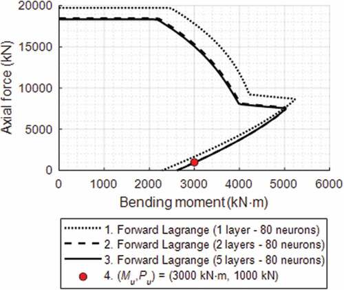
The optimal CI_c-based P–M interaction diagrams for RC columns that satisfy various design criteria (Table 4.1(b) and Table 4.2) are plotted on the basis of forward networks, as shown in Figure 6. The P–M diagrams pass through P_u and M_u, as indicated by a solid point. In Figure 6, the P–M diagrams indicated by Legends 1, 2, and 3 were constructed with the parameters shown in the dashed black box in Table 6(a), (b), and (c), respectively, which were obtained by AI-based Lagrange optimization. These were used to construct P–M diagrams since the accuracies of the parameters obtained by ANN are acceptable. The P–M diagrams were plotted using AutoCol with appropriate input parameters. The interaction diagrams shown in Figure 6 meet the minimum CI_c, as listed in Table 6. CI_c was optimized by Lagrange multiplier-based forward neural networks with one, two, and five layers and 80 neurons. The dotted curve cannot pass through P_u and M_u (solid point), indicating that the training accuracy of a model with one layer is not sufficient. All three optimized P–M diagrams (Legends 1, 2, and 3) shown in Figure 6 would converge, passing through one P–M diagram when the training accuracies are sufficient.

Figure 6. Axial force–moment (P–M) interaction diagrams for optimal CI_c.

5. Conclusions

This study presents hybrid optimization techniques, with which objective functions are proposed based on ANNs. Lagrange optimization techniques with constraints were implemented to achieve rational engineering decisions and find minimized or maximized design values by solving nonlinear optimization problems under strict constraints, conditions, and requirements imposed by design codes for the design of structural frames such as columns and beams. This study helps engineers make the final design decisions, not on the engineers’ empirical observations but on more rational designs, to meet various design requirements, including code restrictions and/or architectural criteria while the objective parameters, such as cost index (CI_c), CO₂ emissions, and structural weight (W_c), are optimized. The conclusions drawn from the study are as follows:

(1) Constructing objective functions and their derivatives, which is a challenge in the Lagrange multiplier method, can now be generalized to any structural design optimization by using ANN to generate universal AI-based objective functions, Jacobian, and Hessian matrices.

(2) Automatic designs of structural frames are proposed for realistic engineering applications to identify design solutions that optimize all design requirements simultaneously, thereby achieving design decisions not based on engineers’ intuition. The results of the sensitivity analysis of LMM show that the best optimal values based on constraints can be identified for specific situations such as official design codes.

(3) Analytical objective functions were difficult to obtain. This study developed the objective functions for CI_c, CO₂ emissions, and W_c based on AI-based networks to be implemented for LMM to find the optimized solutions.

(4) The Karush–Kuhn–Tucker conditions were considered to account for inequality constraints, leading to automatic designs of structural frames that meet various code restrictions simultaneously.

(5) Optimization process for CI_c was performed, and negligible errors were obtained, which were verified using large structural datasets. Engineering calculations also validated the design accuracies when the optimized CI_c was implemented in the designs.

(6) P–M diagrams were are uniquely designed to optimize columns. The proposed optimization will offer generic designs for many types of structures, including machinery and structural frames.

(7) The AI-based objective functions developed in this study can be implemented in broad areas, including engineering, general science, and economics.

A generalizable optimization method proposed herein can be applied to any optimization problem once a sufficient number of data can be collected for establishing approximated objective functions and other parameters to formulate ANN. New objective functions not only enhance the computational speed compared to conventional software but also produce a generalizable calculation method for Jacobian and Hessian matrices for Lagrange optimization. In future work, comprehensive design optimization of a dynamic design of tall buildings would be performed based on AI-based Lagrange optimization. One concerning problem is that computational time of Lagrange optimization is heavily dependent on quantity of inequality constraints because a number of running case (active inequality) corresponds to combinations of inequality constraints. Likewise, a building design is composed of many design requirements considered as inequality constraints, such as lateral displacement, story drift, design strength of each component, and required total base shears, etc.

Acknowledgments

This work was supported by the National Research Foundation of Korea (NRF) grant funded by the Korean government (MSIT 2019R1A2C2004965).

Disclosure statement

No potential conflict of interest was reported by the author.

Additional information

Funding

This work was supported by the National Research Foundation of Korea (NRF) grant funded by the Korean government [MSIT 2019R1A2C2004965].

Notes on contributors

Won-Kee Hong

Dr. Won-Kee Hong is a Professor of Architectural Engineering at Kyung Hee University. Dr. Hong received his Masters and Ph.D. degrees from UCLA, and he worked for Englelkirk and Hart, Inc. (USA), Nihhon Sekkei (Japan) and Samsung Engineering and Construction Company (Korea) before joining Kyung Hee University (Korea). He also has professional engineering licenses from both Korea and the USA. Dr. Hong has more than 30 years of professional experience in structural engineering. His research interests include new approaches to construction technologies based on value engineering with hybrid composite structures. He has provided many useful solutions to issues in current structural design and construction technologies as a result of his research combining structural engineering with construction technologies. He is the author of numerous papers and patents, both in Korea and the USA. Currently, Dr. Hong is developing new connections that can be used with various types of frames, including hybrid steel–concrete precast composite frames, precast frames and steel frames. These connections would contribute to the modular construction of heavy plant structures and buildings as well. He recently published a book titled as ”Hybrid Composite Precast Systems: Numerical Investigation to Construction„ (Elsevier).

Manh Cuong Nguyen

Manh Cuong Nguyen is currently enrolled as a Combined Master & Ph.D. candidate in the Department of Architectural Engineering at Kyung Hee University, Republic of Korea. His research interest includes precast structures. is currently enrolled as a Combined Master & Ph.D. candidate in the Department of Architectural Engineering at Kyung Hee University, Republic of Korea. His research interest includes precast structures.

References

- Abedini, M., and C. Zhang. 2021. “Dynamic Vulnerability Assessment and Damage Prediction of RC Columns Subjected to Severe Impulsive Loading.” Structural Engineering and Mechanics 77 (4): 441–461. doi:10.12989/sem.2021.77.4.441.
- ACI-318. “Building Code Requirements for Reinforced.” 2014.
- Aghaee, K., M. A. Yazdi, and K. D. Tsavdaridis. 2014. “Mechanical Properties of Structural Lightweight Concrete Reinforced with Waste Steel Wires.” Magazine of Concrete Research 66 (1): 1–9. doi:10.1680/macr.14.00232.
- Awal, A. A., I. A. Shehu, and M. Ismail. 2015. “Effect of Cooling Regime on the Residual Performance of High-volume Palm Oil Fuel Ash Concrete Exposed to High Temperatures.” Construction and Building Materials 98: 875–883. doi:10.1016/j.conbuildmat.2015.09.001.
- Barros, M. H. F. M., R. A. F. Martins, and A. F. M. Barros. 2005. “Cost Optimization of Singly and Doubly Reinforced Concrete Beams with EC2-2001.” Structural and Multidisciplinary Optimization 30 (3): 236–242. doi:10.1007/s00158-005-0516-2.
- Beavis, B., and I. Dobbs. 1990. Optimisation and stability theory for economic analysis .Cambridge University press.
- Bengio, Y., I. Goodfellow, and A. Courville. 2017. Deep Learning. Vol. 1. Massachusetts, USA: MIT press.
- Berrais, A. 1999. “Artificial Neural Networks in Structural Engineering: Concept and Applications.” Engineering Sciences 12: 1.
- Camp, C. V., S. Pezeshk, and H. Hansson. 2003. “Flexural Design of Reinforced Concrete Frames Using a Genetic Algorithm.” Journal of Structural Engineering 129 (1): 105–115. doi:10.1061/(ASCE)0733-9445(2003)129:1(105).
- Fanaie, N., S. Aghajani, and S. Shamloo. 2012. “Theoretical Assessment of Wire Rope Bracing System with Soft Central Cylinder”. Proceedings of the 15th World Conference on Earthquake Engineering. Advances in Structural Engineering
- Fanaie, N., S. Aghajani, and E. A. Dizaj. 2016. “Theoretical Assessment of the Behavior of Cable Bracing System with Central Steel Cylinder.” Advances in Structural Engineering 19 (3): 463–472. doi:10.1177/1369433216630052.
- Heydari, A., and M. Shariati. 2018. “Buckling Analysis of Tapered BDFGM Nano-beam under Variable Axial Compression Resting on Elastic Medium.” Structural Engineering & Mechanics 66 (6): 737–748. doi:10.12989/sem.2018.66.6.737.
- Hoffmann, L. D., and G. L. Bradley. 2004. Calculus for Business, Economics, and the Social and Life Sciences.8th. 575–588. ISBN 0-07-242432–X. New York: McGraw Hill Education
- Hong, W. K. 2019. Hybrid Composite Precast Systems: Numerical Investigation to Construction, 427–478. Kidlington, OX5 1GB, United Kingdom: Woodhead Publishing, Elsevier
- Kalman, D. 2009. “Leveling with Lagrange: An Alternate View of Constrained Optimization.” Mathematics Magazine 82 (3): 186–196. doi:10.1080/0025570X.2009.11953617.
- Kaveh, A., and F. Shokohi. 2015. “Optimum Design of Laterally Supported Castellated Beams Using CBO Algorithm.” Steel & Composite Structures 18 (2): 305–324. doi:10.12989/scs.2015.18.2.305.
- Korouzhdeh, T., H. Eskandari-Naddaf, and M. Gharouni-Nik. 2017. “An Improved Ant Colony Model for Cost Optimization of Composite Beams.” Applied Artificial Intelligence 31 (1): 44–63. doi:10.1080/08839514.2017.1296681.
- Madadi, A., H. Eskandari-Naddaf, R. Shadnia, and L. Zhang. 2018. “Characterization of Ferrocement Slab Panels Containing Lightweight Expanded Clay Aggregate Using Digital Image Correlation Technique.” Construction and Building Materials 180: 464–476. doi:10.1016/j.conbuildmat.2018.06.024.
- MATLAB. 2020b. Version 9.9.0 (R2020b). Natick, Massachusetts: MathWorks .
- Nasrollahi, S., S. Maleki, M. Shariati, A. Marto, and M. Khorami. 2018. “Investigation of Pipe Shear Connectors Using Push Out Test.” Steel & Composite Structures 27 (5): 537–543. doi:10.12989/scs.2018.27.5.537.
- Paknahad, M., M. Bazzaz, and M. Khorami. 2018. “Shear Capacity Equation for Channel Shear Connectors in Steel-concrete Composite Beams.” Steel & Composite Structures 28 (4): 483–494. doi:10.12989/scs.2018.28.4.483.
- Protter, M. H., and C. B. Morrey Jr. 1985. Intermediate Calculus. 2nd. 267. New York: Springer.ISBN 0-387-96058-9.
- Rajeev, S., and C. S. Krishnamoorthy. 1998. “Genetic Algorithm–based Methodology for Design Optimization of Reinforced Concrete Frames.” Computer-Aided Civil and Infrastructure Engineering 13 (1): 63–74. doi:10.1111/0885-9507.00086.
- Ripley, B. D. “Pattern Classification and Neural Networks.” 1996.
- Safa, M., M. Shariati, Z. Ibrahim, A. Toghroli, S. B. Baharom, N. M. Nor, and D. Petkovic. 2016. “Potential of Adaptive Neuro Fuzzy Inference System for Evaluating the Factors Affecting Steel-concrete Composite Beam’s Shear Strength.” Steel & Composite Structures 21 (3): 679–688. doi:10.12989/scs.2016.21.3.679.
- Shah, S. N. R., N. R. Sulong, R. Khan, M. Z. Jumaat, and M. Shariati. 2016. “Behavior of Industrial Steel Rack Connections.” Mechanical Systems and Signal Processing 70-71: 25–740. doi:10.12989/scs.2016.21.3.679.
- Shariat, M., M. Shariati, A. Madadi, and K. Wakil. 2018. “Computational Lagrangian Multiplier Method by Using for Optimization and Sensitivity Analysis of Rectangular Reinforced Concrete Beams.” Steel & Composite Structures 29 (2): 243–256. doi:10.12989/scs.2018.29.2.243.
- Shariati, M., S. N. H. Ramli, S. Maleki, and K. M. M. Arabnejad “Experimental and Analytical Study on Channel Shear Connectors in Light Weight Aggregate Concrete.” Proceedings of the 4th International Conference on Steel & Composite Structures. Sydney, Autralia. 2010; 21–23. 1 0.3 850/978-981-08-6218-3_CC-Fr031.
- Silberberg, E., and S. Wing. 2001. The Structure of Economics: A Mathematical Analysis. Third. 134–141. Boston: Irwin McGraw-Hill.ISBN 0-07-234352-4
- Sun, L., Z. Yang, Q. Jin, and W. Yan. 2020. “Effect of Axial Compression Ratio on Seismic Behavior of GFRP Reinforced Concrete Columns.” International Journal of Structural Stability and Dynamics 20 (6): 2040004. doi:10.1142/S0219455420400040.
- Toghroli, A., M. Mohammadhassani, M. Suhatril, M. Shariati, and Z. Ibrahim. 2014. “Prediction of Shear Capacity of Channel Shear Connectors Using the ANFIS Model.” Steel & Composite Structures 17 (5): 623–639. doi:10.12989/scs.2014.17.5.623.
- Villarrubia, G., J. F. De Paz, P. Chamoso, and F. De la Prieta. 2018. “Artificial Neural Networks Used in Optimization Problems.” Neurocomputing 272: 10–16. doi:10.1016/j.neucom.2017.04.075.
- Walsh, G. R. 1975. Saddle-point Property of Lagrangian Function. Methods of Optimization. 39–44. New York:John Wiley & Sons. ISBN 0-471-91922-5.
- Yazdani, M., A. Fakhimi, and M. Alitalesh (2018). “Numerical Analysis of Effective Parameters in Direct Shear Test by Hybrid Discrete–finite Element Method.”
- Ye, M., J. Jiang, H. M. Chen, H. Y. Zhou, and D. D. Song. 2021. “Seismic Behavior of an Innovative Hybrid Beam-column Connection for Precast Concrete Structures.” Engineering Structures 227: 111436. doi:10.1016/j.engstruct.2020.111436.
- Zhang, C., G. Gholipour, and A. A. Mousavi. 2021. “State-of-the-Art Review on Responses of RC Structures Subjected to Lateral Impact Loads.” Arch Computat Methods Eng 28: 2477–2507. doi:10.1007/s11831-020-09467-5.
- Zhang, C., Z. Alam, L. Sun, Z. Su, and B. Samali. 2019. “Fibre Bragg Grating Sensor‐based Damage Response Monitoring of an Asymmetric Reinforced Concrete Shear Wall Structure Subjected to Progressive Seismic Loads.” Structural Control & Health Monitoring 26 (3): e2307. doi:10.1002/stc.2307.