A study of the dynamic seismic performance index of building in Indonesia

ABSTRACT

Recent earthquakes have exposed the vulnerability of buildings in Indonesia. An evaluation is needed to confirm the seismic performance of the structures. A seismic index is a method to determine building performance. This research aims to evaluate the performance using a dynamic seismic performance index _dI_s by considering Indonesia’s seismic hazard. The nonlinear incremental dynamic analysis with a bilinear hysteretic model was used in the analysis. The estimation method using the equivalent linearization and using the characteristic displacement response is proposed to estimate a dynamic ductility index _dF. The dynamic seismic performance index tends to increase with an increase in the critical ductility factor. The dynamic ductility index _dF represents a modification factor (R) that also increases with an increase in the critical ductility. The accuracy of the equivalent linearization is more accurate in the lower period, but the characteristic displacement method gives the closest estimate in the higher period.

KEYWORDS:

• Earthquake
• nonlinear analysis
• dynamic seismic index
• ductility

1. Introduction

Indonesia is an earthquake-prone country that often experiences earthquakes. The main cause is that it is located on the interface of three tectonic plates: Eurasian, Pacific, and Indo-Australian. These plates continue to move and collide with each other. A series of earthquake events have occurred in Indonesia, such as the 1797 collision of the Sumatran-Andaman plate, with a magnitude of 8.9. In 2004, a huge earthquake occurred in Simeulue Island, Banda Aceh, with a magnitude of 9.1 and was followed by a devastating tsunami. There was an earthquake of magnitude 8.5 in Mentawai island in September 2007, and an earthquake of magnitude 7.6 hit Padang in 2009 due to the subducting plate and caused considerable damage to the city. Again on Mentawai island, an earthquake of magnitude 7.8 occurred in 2010, which caused a tsunami on the west coast of those islands (Kurniawandy et al. 2017; Kurniawandy and Nakazawa 2019).

A standard for the seismic evaluation of an existing building was published by The Japan Building Disaster Prevention Association (JBDPA) (Building Research Institute 2017; Kassem, Mohamed Nazri, and Noroozinejad Farsangi 2020). From this, an index to determine buildings’ performance due to earthquake loads, known as the seismic index, was created and is widely used in Japan. Nakazawa et al. (Nakazawa, Yanagisawa, and Kato 2013; Nakazawa and Maeda 2017) proposed a seismic performance evaluation method for steel gymnasiums using a dynamic structural seismic index corresponding to the critical deformation of a member based on the nonlinear seismic response analysis. This method has a more complex analysis in determining the performance index than the seismic index of the JBDPA (Kurniawandy and Nakazawa 2019, 2020), which determined their index without performing dynamic analysis.

So far, there have been no guidelines that can be used to evaluate the performance of an existing structure in Indonesia, although regulations regarding the design of earthquake-resistant structures continue to be updated (Irsyam et al. 2017; Kencanawati, Agustawijaya, and Taruna 2020). This paper proposes a method to obtain the performance of an existing structure with the dynamic seismic index dIs considering Indonesia’s seismic hazard and the dynamic ductility index _dF that represents a modification factor (R). To estimate the dynamic ductility factor, dF, two methods are proposed. The first is the average energy principle with a constant value of 1.0, and the average energy and displacement principle. The second is the equivalent linearization method by considering Indonesia’s response spectrum design.

2. Methodology

In the past, a lot of buildings collapsed during an earthquake, with the ground floor being destroyed while the above floor still existed. This kind of collapse is known as a soft-story phenomenon. In a multi-story building where the upper level is more rigid than the first floor, plastic hinges will occur at the top column, as shown in Figure 1.a. A lumped mass method may be used to model the 3D structures in which the mass is concentrated in the center of mass. The collapse and inter-story drift mechanism of the MDOF system that is dominant in the first mode can be presented in an SDOF system. In this study, the soft-story phenomenon where the adjacent floor is stiffer than the first floor is modeled as an SDOF system for simplification as shown in Figure 1.b. The effective weight and the stiffness of the SDOF system can vary by setting the parameters of the fundamental period T₀, which are selected from 0.1 to 2.0. The yield shear force coefficient C_y varies from 0.1 to 0.5. The critical ductility factor μ_cr is taken from low ductility until high ductility with μ_cr of 1.0 until 10. In order to get nonlinear conditions, seismic intensity λ_E increases step by step from 1.0 until 10 or more, in increments of 1.0. Nonlinear behavior is modeled as a bilinear hysteretic model, which assumes a second stiffness ratio k₂ of 0.05.

Figure 1. SDOF system with bilinear hysteretic model.

The dynamic response characteristic of inelastic systems with respect to earthquake ground motion is one of the fundamental themes in the earthquake-resistant structure design. The nonlinear analysis was carried out, varying the magnitude of the maximum input ground motion by certain increments to measure the continuous response from elastic to yield until nonlinear conditions were reached. This method, known as incremental dynamic analysis, has been used in the previous research (Chomchuen and Boonyapiny 2017; Javanpour and Zarfam 2017; Farzampour, Mansouri, and Dehghani 2019). The dynamic seismic index is obtained from an incremental dynamic analysis that shows the response of a structure as performance due to earthquake load.

In this study, the first step was carried out by a simulated ground motion that fit into Indonesia’s seismic condition and conformed to Indonesia’s seismic code (Indonesian code 2012, 2019). Then, the dynamic analysis was performed using these simulated ground motions. A shear force coefficient at elastic condition (C₀) was calculated by linear dynamic analysis at a seismic intensity (λ_E) of 1.0. In the next stage, the nonlinear dynamic analysis was carried out by increasing the maximum ground acceleration (A_max) by amplifying λ_E with an increment of 1.0 for each step. This was conducted 20 times or more until each model reached a nonlinear condition. Afterward, a linear interpolation was calculated to get the response for each critical ductility (μ_cr) to obtain the result of the dynamic seismic index (_dI_s) and the ductility index (_dF). Each of the above calculations was carried out on each earthquake ground motions.

A total of 1500 combination analyses were carried out by nonlinear dynamic methods, as tabulated in Table 1. The value of the fundamental period (T₀) depends on the stiffness and mass. In general, the low rise and high rise buildings except the base isolation structure will have a period in the range of 0.1 to 2.0 seconds. Earthquake resistant buildings have inelastic state design that generally uses response modification coefficient (R) values ranging from 2.0 to 8.0 based on code. The shear force coefficient at the initial yield (C_y) is the ratio of the maximum shear coefficient at the elastic condition (C_e) and the response modification. It can be expressed as C_y = C_e/R. The value of the shear coefficient can be calculated from the elastic response spectrum based on code. If the structure is at the elastic condition with C_e equal to 1.0 and R = 2.0, so C_y will be 0.5. The C_y value will be less than 0.5 for R = 8.0. When the structure is designed at the inelastic condition, then the value of C_e will be smaller, so the C_y value will be smaller as well. In this study, the C_y value is taken in the range of 0.1 to 0.5.

Table 1. Selected ductility factor when varying T₀ and C_y.

Cy T0	0.1	0.2	0.3	0.4	0.5
0.1	1, 2, 3, ⋯, 10	1, 2, 3, ⋯, 10	1, 2, 3, ⋯, 10	1, 2, 3, ⋯, 10	1, 2, 3, ⋯, 10
0.2	1, 2, 3, ⋯, 10	1, 2, 3, ⋯, 10	1, 2, 3, ⋯, 10	1, 2, 3, ⋯, 10	1, 2, 3, ⋯, 10
⋮	1, 2, 3, ⋯, 10	1, 2, 3, ⋯, 10	1, 2, 3, ⋯, 10	1, 2, 3, ⋯, 10	1, 2, 3, ⋯, 10
1.0	1, 2, 3, ⋯, 10	1, 2, 3, ⋯, 10	1, 2, 3, ⋯, 10	1, 2, 3, ⋯, 10	1, 2, 3, ⋯, 10
1.2	1, 2, 3, ⋯, 10	1, 2, 3, ⋯, 10	1, 2, 3, ⋯, 10	1, 2, 3, ⋯, 10	1, 2, 3, ⋯, 10
⋮	1, 2, 3, ⋯, 10	1, 2, 3, ⋯, 10	1, 2, 3, ⋯, 10	1, 2, 3, ⋯, 10	1, 2, 3, ⋯, 10
2.0	1, 2, 3, ⋯, 10	1, 2, 3, ⋯, 10	1, 2, 3, ⋯, 10	1, 2, 3, ⋯, 10	1, 2, 3, ⋯, 10

Note: 1, 2, 3, ⋯, 10 are μ_cr

2.1. Input earthquake motions

The objective buildings were assumed to be located in Padang city, Indonesia. The demand acceleration spectrum SA at the ground surface is determined by the Indonesian code and is considered as:

(1) $S_A\left(T,h,{\lambda }_E\right)={\lambda }_E\times S_{A0}\left(T\right)\times F_h\left(h\right)$(1)

in which T was the natural period of the structure, h was the damping factor, λE was seismic intensity. This gave an index representing the strength of an earthquake’s ground motion. λE = 1.0 represents a design basis earthquake (DBE) level and corresponds to an extremely rare earthquake with a return period interval of 500 years, while λE = 1.5 represents a risk-targeted maximum considered earthquake (MCER) level and corresponds to the largest possible earthquake expected to occur in the next 2,500 years.

F_h(h) is a numerical coefficient of the response spectrum reduction corresponding to the damping factor h of a structure. Various equations have been proposed for F_h(h). The building standard law (BSL) of Japan (Yenidogan 2016; Yu et al. 2016), adopted the following equation:

(2) $F_h\left(h\right)=\frac{1.5}{1+10.h}$(2)

The Architectural Institute of Japan (AIJ) (Nakazawa and Maeda 2017) recommends the following equation, where a is 75 and h₀ is 5% as initial elastic damping:

(3) $F_h\left(h\right)=\sqrt{\frac{1+a.h_0}{1+a.h_{eq}}}$(3)

The International Building Code (IBC) (Mayes and Naem 2001; ASCE 7-16 2017) proposed a very close approximation to the reduction coefficient related to the damping ratio (h) in the following equation:

(4) $F_h\left(h\right)=0.25\left(1-lnh\right)$(4)

S_A0(T) is a demand acceleration response spectrum with λE = 1.0 and damping factor h = 5% at the ground surface and takes into account the amplification of the surface soil layer.

(5) $S_{A0}\left(T\right)=\left\{\begin{array}{cc}{S}_{DS}\left(0.4+0.6\frac{T}{T_0}\right)& ,T\le T_0\\ S_{DS}& ,T_0<T\le \\ \frac{S_{D1}}{T}& ,T>T_s\end{array}\right.T_s$(5)

; $T_0=0.2\frac{S_{D1}}{S_{DS}}$,$T_S=\frac{S_{D1}}{S_{DS}}$

Here, SD1 is the design spectral response acceleration parameter at 1.0 second, and SDS is the design spectral response acceleration parameter at short periods. Figure 2 shows the design response spectrum as it conforms to SNI 1726 (Indonesian code).

Figure 2. The response spectrum design of Indonesian code.

In order to carry out the time history nonlinear seismic response analysis, the ground motions were simulated to fit the target design of the response spectrum by referring to Equation (5)(5) $S_{A0}\left(T\right)=\left\{\begin{array}{cc}{S}_{DS}\left(0.4+0.6\frac{T}{T_0}\right)& ,T\le T_0\\ S_{DS}& ,T_0<T\le \\ \frac{S_{D1}}{T}& ,T>T_s\end{array}\right.T_s$(5) .

2.2. Simulated ground motions

A nonlinear dynamic method performs analysis with subjected to earthquake ground motions to obtain the result on forces and displacements. The calculation response can be sensitive to the characteristics of single ground motion, so more than ground motion was required (Bybordiani 2018; Mulchandani et al. 2018; Cavdar, Ozdemir, and Bayhan 2019). In the Indonesian code, it is specified that the dynamic analysts must use at least three ground motion data. Indonesia has no recorded the ground acceleration time history for the strong earthquakes that ever occurred. The ground acceleration record can be selected from events of magnitudes that comply with the maximum considered earthquake of Indonesian code. Six ground motion consisting of El-Centro, Kobe, and Taft waves in both directions were used as input ground motion in this analysis. The average of these six data must be close to the response spectrum target.

In order to meet the target of peak ground acceleration (PGA) conforming to the code, a simulated ground motion method was used for scaling the PGA of earthquake data to be equal with PGA in a certain location in Indonesia. The results of the simulated earthquake ground motions were used as the input of seismic loads for dynamic analysis. One target of a response spectrum for simulation is Padang city, located in the west part of Indonesia, because this is the most earthquake-prone city in Indonesia. The risk-targeted maximum considered earthquake (MCER) had an acceleration of 1.39 over a short period (Ss) and 0.6 at the 1.0 second period of period (S₁). The site soil properties were soft soil, and the site coefficients were 0.9 in the short period and 2.4 at the 1.0 second period. Therefore, in the DBE level, the response spectra design at the short period (S_DS) became 0.834 second and 0.96 at the 1.0 second period (S_D1). Results of the simulated peak ground motion can be seen in Table 2.

Table 2. Simulated earthquake ground motions.

Type of Ground Motion	Year	PGA [cm/s^2]	Simulated PGA [cm/s^2]
El Centro – NS	1940	341.6	309.2
El Centro – EW		210.1	259.9
Kobe – NS	1995	817.8	403.0
Kobe – EW		617.1	418.3
Taft – NS	1952	152.7	362.9
Taft – EW		175.9	310.5

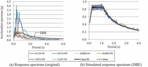
The simulated ground motions of El Centro, Kobe, and Taft earthquakes were scaled into the Indonesia response spectrum, as shown in Figure 3. Figure 3(a) shows the acceleration response spectrum based on the original earthquake motions, and Figure 3(b) shows the acceleration response spectrum based on the simulated earthquake motions at the design basis earthquake (DBE) level. The simulated earthquake motions will be used in every dynamic analysis in this study.

Figure 3. Simulation of the acceleration response spectrum.

2.3. Dynamic seismic index and ductility index

Seismic intensity λ_E is represented as an index identifying the magnitude of the seismic input wave to the objective structure. The maximum input ground acceleration A_max is defined as an index representing the magnitude of the input seismic motion to the objective structure. Nonlinear response analyses were performed while gradually increasing the seismic intensity, and the maximum deformation of the objective structure for each input level was calculated. Figure 4 shows the concept of a dynamic ductility index and dynamic seismic performance index. The relationship between shear force Q (shear force coefficient C) and maximum deformation δ_max (ductility factor μ) is shown.

Figure 4. Relationship between shear force coefficient C and ductility factor μ.

As illustrated in Figure 4, the critical deformation is defined in order to evaluate the limit state of structures. The critical seismic intensity λ_E^cr is obtained when the maximum deformation reaches the critical deformation by nonlinear analysis method. A shear force coefficient at elastic condition C₀ is obtained with respect to λ_E^cr = 1.0. The maximum of shear force coefficient at elastic condition C_e, as expressed as a dynamic seismic performance index _dI_s, corresponding to λ_E^cr, when the structure is elastic, can be expressed as

(6) $C_e={\hspace{0.17em}}_d^{\hspace{0.17em}}{I}_s={\lambda }_E^{cr}{C}_0$(6)

The response modification factor (R) of a structure can be estimated not only from the code of a building’s seismic design but also from dynamic analysis. The dynamic ductility index _dF represents the R-value, which explains the initial yield’s margin to the limit state. The value of _dF is determined by the dynamic seismic index _dI_s dividing the yielding shear coefficient C_y.

(7) ${\hspace{0.17em}}_d^{\hspace{0.17em}}F=\frac{{\hspace{0.17em}}_d^{\hspace{0.17em}}{I}_s}{C_y}=\frac{{\lambda }_E^{cr}\cdot C_0}{C_y}$(7)

In general, the value of C_y is a shear force coefficient corresponding to the ultimate shearing force of a structure.

2.4. Estimation method of ductility index

The dynamic ductility index can be estimated without conducting a dynamic analysis. Two methods were investigated in this paper. The first method was based on the characteristic of maximum displacement, and the second on the equivalent linearization of nonlinear response.

2.4.1. The characteristic displacement response method

The value of the dynamic ductility index can be estimated based on the characteristic of maximum displacement response. The values of _dF are highly dependent on the critical deformation or critical ductility factor μ_cr. In previous studies, Newmark & Hall (Patel and Vyas 2017; Thuat, Van, Chuong, and Duong 2020) proposed rules concerning the relation of maximum displacement and yield strength on the inelastic earthquake response of bilinear systems, as shown in Figure 5. Over a relatively short period, the maximum potential energy of an elastic system (area OAD in Figure 5(a)) and the inelastic potential energy for a system with the same initial period (area OBCE in Figure 5(a)), are almost the same irrespective of the yield strength. This is called the constant energy principle. The relationship of ductility index is closer to:

(8) $F=\frac{Q_e}{Q_y}=\sqrt{2\mu -1}$(8)

Over a relatively long period, the maximum displacement of inelastic systems and the maximum displacement of elastic systems in the same initial period are almost the same if the yield strength is larger than a certain limiting value. This is called the constant displacement principle or property of displacement conservation. The ductility index equation as follows:

(9) $F=\frac{Q_e}{Q_y}=\mu$(9)

For a structure with a very short period, the maximum displacement of systems is an elastic condition. The ductility is ineffective in reducing the required elastic seismic force. The ductility index is a constant of 1.0.

Figure 5. Characteristics of maximum displacement.

This study proposes a transition estimation formula that has a period in between the very short period and short period range. The transition estimation forecasts an average value of the constant energy principle and constant ductility index of 1.0 as follows:

(10) $F=\frac{Q_e}{Q_y}=\left(1+\sqrt{2{\mu }_{cr}-1}\right)/2$(10)

The transition estimation of the ductility index is also proposed for the period range in between a short period and long period. The forecast formula is an average value of the constant energy principle and constant displacement principle as follows:

(11) $F=\frac{Q_e}{Q_y}=\left({\mu }_{cr}+\sqrt{2{\mu }_{cr}-1}\right)/2$(11)

2.4.2. The equivalent linearization method

In 2017, Nakazawa et al. (Nakazawa and Maeda 2017), investigated an estimation method to obtain a seismic performance index for a steel gymnasium structure using the Japanese seismic code. The implementation of this method needed adjustment for the Indonesian seismic code. In this study, the equivalent linearization method proposed by changes the response spectrum parameter by using Indonesia response spectrum design as described in Eq. (5)(5) $S_{A0}\left(T\right)=\left\{\begin{array}{cc}{S}_{DS}\left(0.4+0.6\frac{T}{T_0}\right)& ,T\le T_0\\ S_{DS}& ,T_0<T\le \\ \frac{S_{D1}}{T}& ,T>T_s\end{array}\right.T_s$(5) .

The maximum deformation δmax base on the equivalent linearization method, considering the seismic intensity λ_E can be expressed as:

(12) ${\delta }_{max}=\mu \cdot {\delta }_y=S_D\left({\lambda }_E,T_{eq},h_{eq}\right)=\frac{{T_{eq}}^2}{4^2}{\lambda }_E\times S_{AG0}(T_{eq})\times F_h\left(h_{eq}\right)$(12)

Therefore, the equivalent damping factor h_eq and equivalent period T_eq for the bilinear restoring force can be obtained as follows.

$h_{eq}=h_0+\frac{2}{\pi \mu \kappa }ln\left(\frac{1-\kappa +\mu \kappa }{{\mu }^{\kappa }}\right)$,

(13) $T_{eq}=T_{0\cdot }\sqrt{\frac{\mu }{1+\kappa \left(\mu -1\right)}}$(13)

The critical seismic intensity λ_E^cr corresponding to the critical ductility factor μ_cr is given as

(14) ${\lambda }_E^{cr}=\frac{g{C}_y{T_0}^2}{S_{AG0}\left(T_{eq}\right)\times F_h\left(h_{eq}\right){T_{eq}}^2}\cdot {\mu }_{cr}$(14)

Also, the base shear coefficient C₀ of the elastic system at the damage limit level (λ_E = 1.0) can be obtained from the following equation using the response spectrum:

(15) $C_0=\frac{S_{AG0}\left(T_0\right)\times F_h\left(h_0\right)}{g}$(15)

Substituting Eq. (14)(14) ${\lambda }_E^{cr}=\frac{g{C}_y{T_0}^2}{S_{AG0}\left(T_{eq}\right)\times F_h\left(h_{eq}\right){T_{eq}}^2}\cdot {\mu }_{cr}$(14) and (15(15) $C_0=\frac{S_{AG0}\left(T_0\right)\times F_h\left(h_0\right)}{g}$(15) ) into the definition of _dF in Eq.(7(7) ${\hspace{0.17em}}_d^{\hspace{0.17em}}F=\frac{{\hspace{0.17em}}_d^{\hspace{0.17em}}{I}_s}{C_y}=\frac{{\lambda }_E^{cr}\cdot C_0}{C_y}$(7) ), the estimated value _dF^est of the dynamic ductility index obtained by the equation as follows

(16) ${\hspace{0.17em}}_d^{\hspace{0.17em}}{F}^{est}=\left(\frac{S_{AG0}\left(T_0\right)}{S_{AG0}\left(T_{eq}\right)}\right)\cdot \left(\frac{F_h\left(h_0\right)}{F_h\left(h_{eq}\right)}\right)\cdot \left(1+\kappa \left({\mu }_{cr}-1\right)\right)$(16)

Here, S_AG0 with respect to T₀ and T_eq is determined based on the acceleration response spectrum design conforming to Indonesia’s seismic code. Several reduction factors for this acceleration, as explained in Eq (2)(2) $F_h\left(h\right)=\frac{1.5}{1+10.h}$(2) ,(3(3) $F_h\left(h\right)=\sqrt{\frac{1+a.h_0}{1+a.h_{eq}}}$(3) ), and (4(4) $F_h\left(h\right)=0.25\left(1-lnh\right)$(4) ), are investigated in this study.

3. Analysis result

3.1. Dynamic seismic index

Dynamic linear analysis with a seismic intensity λE of 1.0 was carried out to obtain the elastic shear force coefficient of C0. C0 is the shear force at λE of 1.0 over the weight of the structure (W) as in the following equation:

(17) $C_0=Q\left({\lambda }_E=1.0\right)/W$(17)

_{The result of C0 is presented in Table 3}.

_{Table 3. The shear coefficient of C0.}

T0	δ max	Q max	C0
(s)	(cm)	(kN)
0.10	0.01	4352.50	0.453
0.20	0.06	5686.83	0.592
0.30	0.13	5642.17	0.587
0.40	0.24	5777.83	0.602
0.50	0.39	6025.17	0.627
0.60	0.59	6301.67	0.656
0.70	0.78	6150.83	0.640
0.80	1.07	6463.00	0.673
0.90	1.28	6124.33	0.638
1.00	1.66	6404.83	0.667
1.20	2.24	6028.67	0.628
1.40	2.43	4790.33	0.499
1.60	2.80	4224.67	0.440
1.80	3.18	3797.83	0.395
2.00	3.54	3420.00	0.356

Figure 6 shows the spectrum of the dynamic seismic index varies in the yield shear force coefficients from 0.1 to 0.5, which is the relationship between natural periods and the dynamic seismic index (dIs) in three range of critical ductility (μcr). Linear interpolation was done to estimate the dIs index at each incremental of μcr.

Figure 6. The spectrum of the dynamic seismic index (_dI_s).

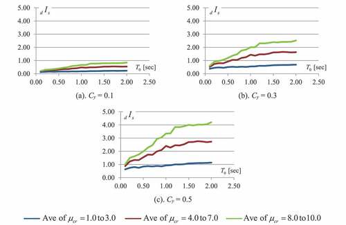
In Figure 6, the values of _dI_s tend to increase with an increasing μ_cr. At low μ_cr, the increase of _dI_s value is not too significant with increasing periods, but it is at higher μ_cr. The yield shear force coefficient C_y will have a significant effect on large of the critical ductility μ_cr.

3.2. Dynamic ductility index

The dynamic ductility index is defined as the ratio between the elastic shear coefficient at the initial yielding C_y and the maximum shear coefficient at elastic condition C_e. Figure 7 shows the relationship between the dynamic ductility index (_dF) and critical ductility (μ_cr) in period of 0.1 to 2.0 second. The periods are divided into three levels: 0.1 to 0.7, 0.8 to 1.4, and 1.5 to 2.0 seconds. The average value represents each level of the period.

Figure 7. Relationship dynamic ductility index (_dF) and critical ductility (μ_cr).

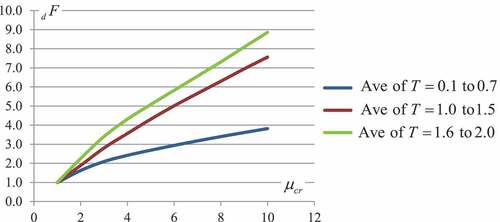
As shown in Figure 7, the value of _dF increases with an increase μ_cr value. The other of C_y’s dynamic ductility index is also generating, and the results show the graph is typical for every C_y value. This indicates that the value of _dF is independent of C_y.

Figure 8. The spectrum of dynamic ductility index (_dF).

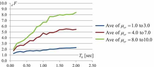
Figure 8 shows the dynamic ductility index spectrum in three range of critical ductility, which data in each range is the average value. These three data show the three levels of critical ductility from the first structure with low critical ductility, then a structure with middle ductility and finally a structure with high critical ductility. The spectrum of _dF for C_y of 0.1, 0.2 0.3, 0.4, and 0.5 are similar to each other due to _dF being independent of C_y. In Figure 8, the structure with high ductility produces greater _dF at a high natural period. On the other hand, a structure with low ductility produces small _dF values over an increasing period.

3.3. Estimation of ductility index

Dynamic analysis was done using a simulated earthquake load based on the Indonesian response spectrum.

3.3.1. Characteristic displacement estimation method

The dynamic ductility index (_dF) for several critical ductility factors (μ_cr) from low to high was calculated. The ductility index was estimated based on the proposal equation (8)(8) $F=\frac{Q_e}{Q_y}=\sqrt{2\mu -1}$(8) ,(9(9) $F=\frac{Q_e}{Q_y}=\mu$(9) ),(10(10) $F=\frac{Q_e}{Q_y}=\left(1+\sqrt{2{\mu }_{cr}-1}\right)/2$(10) ), and (11(11) $F=\frac{Q_e}{Q_y}=\left({\mu }_{cr}+\sqrt{2{\mu }_{cr}-1}\right)/2$(11) ) as follows:

${\hspace{0.17em}}_d^{\hspace{0.17em}}{F}_{est\mathrm{\_}1}=\sqrt{2{\mu }_{cr}-1}$

${\hspace{0.17em}}_d^{\hspace{0.17em}}{F}_{est\mathrm{\_}2}=\mu { }_{cr}$

${\hspace{0.17em}}_d^{\hspace{0.17em}}{F}_{est\mathrm{\_}3}=\left(1+\sqrt{2{\mu }_{cr}-1}\right)/2$

(18) ${\hspace{0.17em}}_d^{\hspace{0.17em}}{F}_{est\mathrm{\_}4}=\left({ }_{cr}+\sqrt{2{\mu }_{cr}-1}\right)/2$(18)

The ratio of dynamic ductility index (_dF) and estimated ductility index (_dF_est) was obtained in order to observe the accuracy of the estimation. When the ratio of _dF/_dF_est was close to 1.0, it meant that the estimation was more accurate from being greater or lower than one. A horizontal line marker, which has a constant gradient of 1.0, was plotted to mark the accuracy of the ratio.

Figure 9. The reliability of the ductility index estimation method with increasing the critical ductility factor.

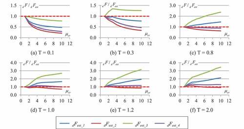
Figure 9 shows the relationship between the critical ductility factor (μ_cr) and the ratio of _dF/_dF_est . As shown in Figure 9.a, at a period of 0.1, the chart of _dF_{est_3} is close to the horizontal line of 1.0 compared to the other charts. However, the estimation method changed at period 0.3, and the chart of _dF_{est_1} was closer than the others (Figure 9.b). In Figure 9.c, the estimation of _dF_{est_4} was closer to the horizontal line. The estimation of _dF_{est_2} was closer from 1.2 up to 2.0 (Figure 9.e and 9.f).

The accuracy of all estimation methods, as shown in Figure 9, is summarised in Table 4. An average error for the whole critical ductility (μ_cr) was calculated for each period. The accurate estimation method was selected based on minimum error. Table 4 shows the minimum error for each estimation method.

Table 4. The percentage of error estimation for each _dF estimation.

T0	% Error					dFest_#
	dFest_1	dFest_2	dFest_3	dFest_4	Min
0.1	38.7%	58.7%	13.8%	51.6%	13.8%	dFest_3
0.2	19.1%	47.4%	16.0%	37.4%	16.0%	dFest_3
0.3	12.9%	43.6%	25.3%	32.8%	12.9%	dFest_1
0.4	12.8%	44.3%	26.0%	33.2%	12.8%	dFest_1
0.5	1.0%	37.2%	43.5%	24.5%	1.0%	dFest_1
0.6	9.1%	31.7%	59.1%	17.4%	9.1%	dFest_1
0.7	10.4%	31.5%	61.6%	16.9%	10.4%	dFest_1
0.8	24.8%	23.7%	83.9%	6.9%	6.9%	dFest_4
0.9	28.1%	22.3%	89.3%	4.9%	4.9%	dFest_4
1.0	42.4%	14.1%	111.0%	5.5%	5.5%	dFest_4
1.1	39.6%	15.7%	106.8%	3.4%	3.4%	dFest_4
1.2	53.2%	8.1%	127.6%	13.1%	8.1%	dFest_2
1.3	52.5%	8.7%	126.5%	12.4%	8.7%	dFest_2
1.4	56.6%	6.2%	132.7%	15.5%	6.2%	dFest_2
1.5	64.1%	1.6%	143.8%	21.1%	1.6%	dFest_2
1.6	63.9%	1.6%	143.5%	21.1%	1.6%	dFest_2
1.7	66.7%	0.0%	147.7%	23.1%	0.0%	dFest_2
1.8	66.1%	0.3%	146.7%	22.7%	0.3%	dFest_2
1.9	65.7%	0.5%	146.2%	22.4%	0.5%	dFest_2
2.0	69.5%	1.5%	151.9%	25.0%	1.5%	dFest_2

From Table 4, the estimation of the ductility index, _dF_est, can be formulated with respect to the range of period shown in this following equation:

(19) ${\hspace{0.17em}}_d^{\hspace{0.17em}}{F}^{est}=\left\{\begin{array}{cc}1& ,T<0.1\\ \left(1+\sqrt{2{\mu }_{cr}-1}\right)/2& ,0.1\le T<0.3\\ \sqrt{2{\mu }_{cr}-1}& ,0.3\le T<0.8\\ \left({\mu }_{cr}+\sqrt{2{\mu }_{cr}-1}\right)/2& ,0.8\le T<1.2\\ {\mu }_{cr}& ,1.2\le T<2.0\end{array}\right.$(19)

Equation (19)(19) ${\hspace{0.17em}}_d^{\hspace{0.17em}}{F}^{est}=\left\{\begin{array}{cc}1& ,T<0.1\\ \left(1+\sqrt{2{\mu }_{cr}-1}\right)/2& ,0.1\le T<0.3\\ \sqrt{2{\mu }_{cr}-1}& ,0.3\le T<0.8\\ \left({\mu }_{cr}+\sqrt{2{\mu }_{cr}-1}\right)/2& ,0.8\le T<1.2\\ {\mu }_{cr}& ,1.2\le T<2.0\end{array}\right.$(19) consists of 5 groups covering different periods. The first group is for a period of less than 0.1. The ductility index can be estimated with a constant value of 0.1. In the second group, for a period between 0.1 and 0.3, the ductility index can be estimated with the average of energy principle and constant ductility index of 1.0, Eq. (10)(10) $F=\frac{Q_e}{Q_y}=\left(1+\sqrt{2{\mu }_{cr}-1}\right)/2$(10) . The energy principle can estimate the ductility index in the range of 0.3 to 0.8 in the third group. The average of the energy and displacement principle, Eq. (11(11) $F=\frac{Q_e}{Q_y}=\left({\mu }_{cr}+\sqrt{2{\mu }_{cr}-1}\right)/2$(11) ), can estimate the ductility index at 0.8 until less than 1.2 in the fourth group. In the last group, at a period greater than 1.2, the ductility index is close to the critical ductility value, which corresponds to the displacement principle.

3.3.2. Equivalent linearization estimation method

The equivalent linearization method has a numerical coefficient to reduce the response spectrum associated with the structure’s damping factor. This research investigates three methods in determining the reduction factor, Eq.(2(2) $F_h\left(h\right)=\frac{1.5}{1+10.h}$(2) ), Eq.(3(3) $F_h\left(h\right)=\sqrt{\frac{1+a.h_0}{1+a.h_{eq}}}$(3) ), and Eq.(4(4) $F_h\left(h\right)=0.25\left(1-lnh\right)$(4) ), which are compared with the dynamic analysis results. The reliability of the displacement estimation method, Eq.(19)(19) ${\hspace{0.17em}}_d^{\hspace{0.17em}}{F}^{est}=\left\{\begin{array}{cc}1& ,T<0.1\\ \left(1+\sqrt{2{\mu }_{cr}-1}\right)/2& ,0.1\le T<0.3\\ \sqrt{2{\mu }_{cr}-1}& ,0.3\le T<0.8\\ \left({\mu }_{cr}+\sqrt{2{\mu }_{cr}-1}\right)/2& ,0.8\le T<1.2\\ {\mu }_{cr}& ,1.2\le T<2.0\end{array}\right.$(19) is also investigated by comparing it to the linearization method. Figure 10 shows the relationship between the critical ductility factor and the dynamic ductility index at any given period using several estimation methods.

Figure 10. Relationship critical ductility factor and dynamic ductility index on several estimation methods.

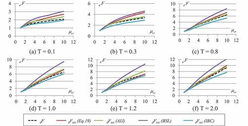
In Figure 10, it can be seen, the estimation method using BSL reduction is at the top of the graph of the dynamic analysis result, which means the estimation is larger than the dynamic ductility index (_dF). Any other way, the estimation using the IBC reduction factor is slightly smaller than _dF. The estimation method using the AIJ reduction factor gives the closest estimate to the dynamic ductility index. To facilitate observation, the estimation error percentage using the AIJ reduction factor by excluding BSL and IBC is compared head-to-head with the characteristic displacement method as per Eq.(19)(19) ${\hspace{0.17em}}_d^{\hspace{0.17em}}{F}^{est}=\left\{\begin{array}{cc}1& ,T<0.1\\ \left(1+\sqrt{2{\mu }_{cr}-1}\right)/2& ,0.1\le T<0.3\\ \sqrt{2{\mu }_{cr}-1}& ,0.3\le T<0.8\\ \left({\mu }_{cr}+\sqrt{2{\mu }_{cr}-1}\right)/2& ,0.8\le T<1.2\\ {\mu }_{cr}& ,1.2\le T<2.0\end{array}\right.$(19) in Table 5.

Table 5. The percentage of error comparison for both estimation method.

T0	% Error		Min error
	dF_est_AIJ	dF_eq(19)	estimation
0.1	9.6%	13.8%	dF_est_AIJ
0.2	3.2%	16.0%	dF_est_AIJ
0.3	3.1%	12.9%	dF_est_AIJ
0.4	2.7%	12.8%	dF_est_AIJ
0.5	7.3%	1.0%	dF_eq(19)
0.6	8.0%	9.1%	dF_est_AIJ
0.7	1.9%	10.4%	dF_est_AIJ
0.8	0.9%	6.9%	dF_est_AIJ
0.9	8.5%	4.9%	dF_eq(19)
1.0	7.9%	5.5%	dF_eq(19)
1.1	16.9%	3.4%	dF_eq(19)
1.2	12.8%	8.1%	dF_eq(19)
1.3	13.3%	8.7%	dF_eq(19)
1.4	11.0%	6.2%	dF_eq(19)
1.5	6.8%	1.6%	dF_eq(19)
1.6	6.9%	1.6%	dF_eq(19)
1.7	5.4%	0.0%	dF_eq(19)
1.8	5.7%	0.3%	dF_eq(19)
1.9	5.8%	0.5%	dF_eq(19)
2.0	3.9%	1.5%	dF_eq(19)

As shown in Table 5, the accuracy using the equivalent linearization method is more accurate for the lower period in the range of 0.1 to 0.8. The average error percentage is about 4.6%, which lower than the displacement estimation method of 10.4%. However, the characteristic displacement estimation method gives the closest estimation for the higher period in the range of 0.9 to 2.0. The average error percentage is about 3.5%, which lower than the equivalent linearization method of 8.7%. Both estimation methods can be used as alternatives to estimate the dynamic ductility index and dynamic seismic index of a structure without carrying out a nonlinear dynamic analysis, which is very complex and takes a long time.

4. Conclusion

This study dealt analytically with the dynamic seismic index _dI_s and the dynamic ductility index _dF with increasing the maximum ground acceleration A_max by amplifying the seismic intensity λ_E in order to evaluate the seismic performance of a structure. The response analysis is performed using simulated earthquake motions that fit the design response spectrum. The paper shows the peak ground acceleration (PGA) of the simulated earthquake motions fit into the design response spectrum conformed to Indonesia’s seismic code as the target. A collection of simulated ground motions was used in linear and nonlinear dynamic analysis. The values of _dI_s and _dF were analyzed for a structure that had critical ductility factor μ_cr at a low ductility and at high ductility.

The relationship between _dI_s and critical ductility factor μ_cr showed that the values of _dI_s tended to increase with increasing μ_cr. Similar to _dI_s, the _dF value increases with an increase in the value of μ_cr, but the _dF is independent of C_y. A structure with a high natural period and high ductility will produce a greater _dF value.

The ductility index can be estimated by the estimation method without conducting the dynamic analysis. Two estimation methods were introduced in this paper. The first was the characteristic displacement response method, formulated from the relationship of the critical ductility factor μ_cr and the ductility index, as shown in equation (19)(19) ${\hspace{0.17em}}_d^{\hspace{0.17em}}{F}^{est}=\left\{\begin{array}{cc}1& ,T<0.1\\ \left(1+\sqrt{2{\mu }_{cr}-1}\right)/2& ,0.1\le T<0.3\\ \sqrt{2{\mu }_{cr}-1}& ,0.3\le T<0.8\\ \left({\mu }_{cr}+\sqrt{2{\mu }_{cr}-1}\right)/2& ,0.8\le T<1.2\\ {\mu }_{cr}& ,1.2\le T<2.0\end{array}\right.$(19) . The second was the equivalent linearization method.

The accuracy of the estimation method using equivalent linearization is more accurate in the lower period. The average error percentage is about 4.6%, which lower than the characteristic displacement estimation method of 10.4%. However, the proposed method using the characteristic displacement estimation response gave the closest estimate in the higher period. The average error percentage is about 3.5%, which lower than the equivalent linearization method of 8.7%.

Disclosure statement

No potential conflict of interest was reported by the author(s).

References

- ASCE 7-16. 2017. Minimum Design Loads and Associated Criteria for Buildings and Other Structures. American Society of Civil Engineers, USA.
- Building Research Institute. 2017. Standard for Seismic Evaluation of Existing Reinforced Concrete Buildings (English Version). Tokyo, Japan: Japan Building Disaster Prevention Association (JBDPA).
- Bybordiani, M. 2018. “Effectiveness of Motion Scaling Procedures for the Seismic Assessment of Concrete Gravity Dams for near Field Motions.” Structure and Infrastructure Engineering 14 (10): 1339–1354. doi:10.1080/15732479.2018.1434210.
- Cavdar, E., G. Ozdemir, and B. Bayhan. 2019. “Significance of Ground Motion Scaling Parameters on Amplitude of Scale Factors and Seismic Response of Short and Long-Period Structures.” Earthquake Spectra 35 (4): 1663–1688. doi:10.1193/081718EQS204M.
- Chomchuen, P., and V. Boonyapiny. 2017. “Incremental Dynamic Analysis with Multi-modes for Seismic Performance Evaluation of RC Bridges.” Engineering Structures 132: 29–43. doi:10.1016/j.engstruct.2016.11.026.
- Farzampour, A., I. Mansouri, and H. Dehghani. 2019. “Incremental Dynamic Analysis for Estimating Seismic Performance of Multi-story Buildings with Butterfly-shaped Structural Dampers.” Buildings 9 (4): 1–10. doi:10.3390/buildings9040078.
- Indonesian code. 2012. SNI 1726: 2012Earthquake Resistant Design Code for Building and non-Building of Indonesia (In Indonesian). Jakarta: Standardization Agency of Indonesia (BSN).
- Indonesian code. 2019. SNI 1726: 2019Earthquake Resistant Design Code for Building and non-Building of Indonesia (In Indonesian). Jakarta: Standardization Agency of Indonesia (BSN).
- Irsyam, M., P. R. Cummins, M. Asrurifak, L. Faizal, D. H. Natawidjaja, S. Widiyantoro, I. Meilano, W. Triyoso, A. Rudiyanto, S. Hidayati, M. Ridwan, N. R. Hanifa, and A. J. Syahbana. 2017. “Development of New Seismic Hazard Maps of Indonesia 2017.” In: Proceedings of the 19th International Conference on Soil Mechanics and Geotechnical Engineering. 1525–1528. Seoul, Korea. doi: 10.1177/8755293020951206.
- Javanpour, M., and P. Zarfam. 2017. “Application of Incremental Dynamic Analysis (IDA) Method for Studying the Dynamic Behavior of Structures during Earthquakes.” Engineering, Technology & Applied Science Research 7 (1): 1338–1344. doi:10.48084/etasr.902.
- Kassem, M. M., F. Mohamed Nazri, and E. Noroozinejad Farsangi. 2020. “The Seismic Vulnerability Assessment Methodologies: A State-of-the-art Review.” Ain Shams Engineering Journal 11 (4): 849–864. doi:10.1016/j.asej.2020.04.001.
- Kencanawati, N. N., D. S. Agustawijaya, and R. M. Taruna. 2020. “An Investigation of Building Seismic Design Parameters in Mataram City Using Lombok Earthquake 2018 Ground Motion.” Journal of Engineering and Technological Sciences 52 (5): 651–664. doi:10.5614/j.eng.technol.sci.2020.52.5.4.
- Kurniawandy, A., S. Nakazawa, A. Hendry, and R. Firdaus. 2017. “Structural Building Screening and Evaluation.” In: International Conference on Civil Engineering, AIP Conference Proceedings 1892. Penang, Malaysia. doi: 10.1063/1.5005662.
- Kurniawandy, A., and S. Nakazawa, 2019. “Seismic Performance Evaluation of Existing Building Using Seismic Index Method”. In: International Conference on Advances in Civil and Environmental Engineering (ICAnCEE 2018). Bali, Indonesia. doi: 10.1051/matecconf/201927601015.
- Kurniawandy, A., and S. Nakazawa. 2020. “A Proposal of Seismic Index for Existing Buildings in Indonesia Using Pushover Analysis.” Journal of Engineering and Technological Sciences 52 (3): 310–330. doi:10.5614/j.eng.technol.sci.2020.52.3.2.
- Mayes,R.L., and F.Naem. 2001. “Design of Structures with Seismic Isolation”. In The Seismic Design Handbook, edited by F. Naeim. US: Springer. doi:10.1007/978-1-4615-1693-4_14.
- Mulchandani, H. K., G. Muthukamar, and S. Bansal. 2018. “Ground Motion Selection and Scaling Using ASCE 7-16, Case Study on Town Alipur in Delhi Region”. In: The 16th Symposium on Earthquake Engineering. India, 1–9.
- Nakazawa, S., and H. Maeda, 2017. “Estimation Method for Dynamic Ductility Index of Steel Structures by Using Equivalent Linearization Method.” In: International Conference on Civil Engineering, AIP Conference Proceedings 1892. Penang, Malaysia. doi: 10.1063/1.5005637.
- Nakazawa, S., T. Yanagisawa, and S. Kato. 2013. “Evaluation of Dynamic Ductility Index of Steel Gymnasiums Based on Pushover Analysis.” Journal of Structural and Construction Engineering (Transaction of AIJ) 78 (683): 111–118. doi:10.3130/aijs.78.11.
- Patel, N. K., and P. Vyas, 2017. “Evaluation of Response Modification Factor for Moment Resisting Frames.” In: International Conference on Research and Innovations in Science, Engineering and Technology ICRISET2017. India, 118–111.
- Thuat, D., H. V. Van, Chuong, and B. Duong. 2020. “Relationship of Strength Reduction Factor and Maximum Ductility Factor for Seismic Design of One‑storey Industrial Steel Frames.” Asian Journal of Civil Engineering 21 (5): 841–856. doi:10.1007/s42107-020-00244-0.
- Yenidogan, C. 2016. “A Comparative Evaluation of Design Provisions for Seismically Isolated Buildings.” Soil Dynamics and Earthquake Engineering 90: 265–286. doi:10.1016/j.soildyn.2016.08.016.
- Yu, G., M. Asce, G. Y. K. Chock, and F. Asce, 2016. “Comparison of the USA, China and Japan Seismic Design Procedures.” In: CECAR7 Civil Engineering Conference in the Asia Region. 1–16. Waikiki, Oahu, Hawaii, USA.