Response modification factor and displacement amplification factor of K-shaped eccentrically braced high-strength steel frames

ABSTRACT

A K-shaped eccentrically braced high-strength steel frame is a novel structure. For such structures to exhibit good plastic deformation under severe earthquakes, the links are made of ordinary steel (fy≤345 MPa), whereas high-strength steel (fy≥460 MPa) is used in the frame beams and columns to reduce the cross section while ensuring the elasticity of the nonenergy consuming components. The response modification factor R is crucial to the performance-based seismic design. For an appropriate and economical seismic design, the R value and displacement amplification factor Cd should be reasonably selected. In China’s code for Seismic Design of Buildings R is uniform without considering high-strength steel, which is unreasonable. It is important to study R and Cd of K-shaped eccentrically braced high-strength steel frame. Therefore, structures with different stories (5, 10, 15, and 20 stories) and link lengths (900, 1000, 1100, and 1200 mm) were designed via the performance-based seismic design method. A static nonlinear pushover analysis and an increment dynamic analysis (IDA) were conducted. The R and Cd of each prototype were calculated using the capacity spectrum method. The effects of various factors in terms of the number of stories and link length were evaluated.

KEYWORDS:

• K-shaped eccentrically braced frame
• high-strength steel frame
• pushover analysis
• increment dynamic analysis
• response modification factor
• displacement amplification factor

1. Introduction

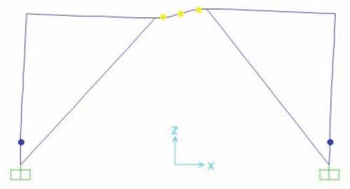
K-shaped eccentrically braced frames (EBFs) made of high-strength steel are a new type of structure, in which an ordinary steel (f_y ≤ 345 MPa) is utilized for the links and braces, whereas a high-strength steel (f_y ≥ 460 MPa) is used for the frame beams and columns, as shown in Figure 1. This type of structure not only reduces the cross-sectional size of the beam and column members, but also promotes the application of high-strength steel in seismic fortification areas. This significantly improves the performance of eccentrically braced steel frames and reduces the cost. The structure relies on the plastic shear deformation of the links to consume the seismic energy under severe earthquake loading, while the beams and columns remain in the elastic state (Li, Su, and Sui 2019).

Conventional design methods lead to structural over-strength, the large section size limits the engineering application of the structure, and the calculation accuracy cannot be ensured (Li, Su, and Lian et al. 2015). Therefore, the design concept of structural energy dissipation proposed by Japanese experts has been widely accepted (Tong and Zhao 2008). Based on the ductility and over-strength of structures, the energy consumption capacity of the structure in the ductile state is fully utilized to allow the structure to enter the elastoplastic range under severe earthquake loading. The response spectrum and displacement are adjusted on the basis of the response modification factor R and displacement amplification factor C_d; thus, the seismic performance of the structure under earthquake loading can be improved (Yang, Gu, and He 2010). Based on the analytically predicted dynamic responses of four actual building frames subjected to a set of eight historical earthquake records, some conclusions were obtained regarding the ratio of the seismic deflection amplification factor to the force reduction factor (Uang and Maarouf 1994). Twelve EBFs of different heights (3, 9, and 18 stories) and strengths were designed, and two types of analyses were performed: a static elastic analysis under the design base shear and a nonlinear dynamic analysis under ten design-level earthquakes. The correlation between the two types of analyses was found to be poor. Calibrated amplification factors were developed to better estimate the link inelastic rotation. Amplifying only the shear component of the elastic story deformations can help obtain more reasonable estimates (Richards and Thompson 2009). Based on the results of a numerical study, a new set of displacement amplification factors was established. With the proposed modifications, the EBFs were redesigned and analyzed using an inelastic time-history analysis. The proposed modifications helped improve the calculation procedures for the displacement amplification factor and link rotation angle (Kuşyılmaz and Topkaya 2014). The response modification factor and displacement amplification factor are vital to the design of steel and concrete structures. In seismic design, the response modification factor is typically used to reduce the structural strength under seismic fortification and to further calculate its seismic response (Yang et al., 2012). The displacement amplification factor is used to amplify the displacement in the elastic range so that the plastic displacement and deformation capacity of the structure can be estimated. Therefore, the response modification factor and displacement amplification factor are key considerations in the seismic design. The values of the two factors are directly related to the safety and performance of the structure during an earthquake. In recent years, some countries have proposed specifications for the response modification factor and displacement amplification factor; however, the values under these specifications are different. Because of empirical differences, the R and C_d values are not uniform. Any modification to the C_d value makes the link sections to experience a lower degree of link rotation angle during seismic events and exhibit stiffening, which increase the cumulative link rotation angle capacity, whereas any modification to the R factor can result in inadequate stiffening of the link beams (Kuşyılmaz and Topkaya 2016). R takes a uniform value of 2.8125 as specified in the Code for Seismic Design of Buildings (GB50011-2010 2010). This setting does not distinguish between specific structural forms and yields different R factors. This leads to poor reliability of specific structures and makes some structures unsafe.

Figure 1. Eccentrically braced frame made of a high strength steel.

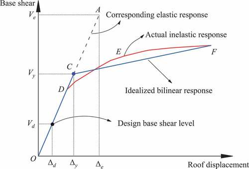
Figure 2. Performance curve of the structure.

The response modification factor is the ratio of the base shear in the fully elastic state under moderate earthquake to the design base shear in the inelastic state under the same seismic level. In the current seismic design code of China, the concept of response modification factor refers to reducing the elastic response spectrum of a single-degree-of-freedom (SDOF) system under moderate earthquakes (Li and Su 2014). Later, scholars have studied and investigated the deflection amplification of buckling-restrained braced frames (BRBFs). The results revealed that the deflection amplification is nonuniform along the building height. Inelastic drifts were found to accumulate in the lower stories, and the deflection amplification factor (C_d) exceeded the recommended value of 5.0 in the ASCE 7 standard. A C_d profile that varies along the building height was proposed, enabling cost-optimized solutions when compared with the use of a single-valued deflection amplification factor (Özkılıç, Bozkurt, and Opkaya 2018). The displacement amplification factor C_d is the ratio of the maximum elastoplastic displacement to the design displacement of the structure at a certain seismic level. In the seismic design of structures, the displacement amplification factor is used to estimate the maximum plastic displacement and to predict their maximum deformation capacity (Su and Li 2014). Researchers have conducted a significant amount of work on the response modification factor and displacement amplification factor of structures such as moment-resisting frames and concentrically braced frames (Lu and Gu 2008). A series of three-story, nine-story, and 20-story special concentrically braced frames (SCBFs) were designed and evaluated. The results showed significant variation between the FEMAP695 method and an alternate procedure for scaling the multiple acceleration records to the seismic design hazard. Among the buildings studied, the three-story building exhibited the highest vulnerability. To achieve a consistent margin of safety against collapse, a significantly lower R factor is required for low-rise SCBFs (three-story), whereas the current value of 6 can be continued for mid-rise and high-rise SCBFs (9-story and 20-story), as provided in ASCE-07 (Hsiao, Lehman, and Roeder 2013). Scholars have focused on the overall dynamic behavior of moment resisting frames (MRFs), BRBFs, and self-centering buckling-restrained braced frames under pulse-like near-fault earthquakes. To facilitate performance-based design, residual inter-story drift (RID) prediction models have been proposed, enabling a quick evaluation of the relationship between the maximum inter-story drift and the RID (Fang et al. 2018). In accordance with ASCE 7–05, 2–12 story buildings were designed to study the comparative residual drift response of special moment-resisting frames (SMRFs) and BRBFs. BRBFs experience greater residual drifts than SMRFs; however, the scatter in the residual drift results is significant (Erochko et al. 2010). A novel type of self-centering brace called variable friction self-centering energy-dissipation brace (VF-SCEDB) has been proposed, and an experimental study on a proof-of-concept VF-SCEDB specimen was conducted. The proposed VF-SCEDB exhibited both excellent energy-dissipation and self-centering capabilities. Self-centering frames have almost negligible residual inter-story drift under the maximum earthquake considered. Compared with normal SCBs and SCEDBs, the proposed VF-SCEDBs can further reduce the peak deformation and mitigate inter-story drift concentration (Chen et al. 2020). The overstrength, ductility, and response modification factors of low-to-mid-rise BRBFs designed as per the National Building Code of Canada 2010 have been evaluated. Four-, six-, and eight-story buildings with span lengths of 6 m and 8 m were designed and analyzed. The code prescribed value of 4.8 is somewhat a lower bound for the response modification factor of BRBFs. Additionally, the response modification factor decreases with the increase in the story height and span length. The response modification factor may be slightly affected by the bracing configuration (Moni, Moradi, and Alam 2016). The chapter “Seismic design requirements for building structures” in ASCE 7–16 presents the design coefficients and factors for various seismic force-resisting systems. For a particular structure, there is only one set of R and C_d values, e.g., R = 8.0 and C_d = 4.0 for steel EBFs; appropriate values of the response modification coefficient R, overstrength factor Ω₀, and deflection amplification factor C_d are used to determine the base shear, element design forces, and design story drift.

The response modification factor and displacement amplification factor are not specified and are difficult to quantify. There is a lack of understanding of these factors.

The response modification factor R and displacement amplification factor C_d can be determined on the basis of the structural response curve shown in Figure 2 (Uang 1991). The horizontal coordinates in Figure 2 are the roof displacements of the structure, and the vertical coordinates are the base shear. OA is the performance curve of the structure in the perfectly elastic state, ODEF is the actual elastic response of the structure under earthquake loading, and ODCF is the performance curve of the structure in the ideal state. The actual nonlinear response of the structure is idealized by a bilinear elastoplastic relationship (lines ODEF are transferred to ODCF in Figure 2). The bilinear line ODCF coincides with the initial linear response of the structure, and the area enclosed by ODCF is equal to the area under the actual curve.

The response modification factor R is defined as follows:

(1) $R=\frac{V_e}{V_d}=\frac{V_e}{V_y}\times \frac{V_y}{V_d}=R_{\mu }\times R_{\mathrm{\Omega }}$(1)

Here, the ductility reduction factor R_μ is a parameter that measures the strength reduction due to the inelasticity effect, R_μ = V_e/V_y, where V_e is the maximum seismic demand for an elastic response, and V_y is the base shear corresponding to the maximum inelastic displacement and is also the yield force of the structure; R_Ω is the over-strength factor defined as the ratio of V_y to the design base shear V_d (R_Ω = V_y/V_d). The calculation formula for the displacement amplification factor C_d is:

(2) $C_d=\frac{{\mathrm{\Delta }}_{max}}{{\mathrm{\Delta }}_d}$(2)

where Δ_max is the maximum displacement of the structure under moderate or severe seismic ground motion, and Δ_d is the design roof displacement of the structure.

In this study, the response modification factor and displacement amplification factor of a K-shaped eccentrically braced high-strength steel frame were analyzed. Our results will not only help optimize the seismic performance of this new structure and improve its safety and applicability from an economic perspective, but also help develop the design theory of existing seismic specifications. Thus, a reference is provided for the seismic design of this type of structural system.

2. Structural design and finite element modeling

2.1. Performance-based seismic design (PBSD)

The target drift and expected failure mode are primarily determined when designing a structure through the PBSD method. For EBFs, the expected failure mode is when only the links dissipate energy while the other components remain elastic when the structure is being loaded in the elastoplastic state. The story drifts along the height of the structure are well-distributed.

For EBFs, the steps involved in the PBSD method are as follows:

1) First, the fundamental period of the EBF structures is estimated, and the yield drift θ_y and target drift θ_u of the EBFs are calculated using approximate formulae. The ductility factor μ_s = θ_u/θ_y and ductility reduction factor R_μ are acquired using μ_s.

2) Second, the base shear-to-structure weight ratio V/G in the elastoplastic state is calculated using the ductility factor and other parameters, and the base shear force in the elastoplastic state is obtained.

3) Third, the story shear force of each story is obtained via the shear force distribution in the elastoplastic state. β_i represents the shear distribution factor at level i, which is equal to V_i/V_n.

4) The link design is a key procedure in the PBSD method, because plastic deformations are isolated in the links and column bases. When the lateral force distribution is known, yield shear links are proportioned to create a uniform story drift along the height. By using the principle of virtual work and equating the external work to the internal work, the section of shear links can be determined.

5) Finally, the other members, such as braces, beams, and columns, are confirmed by the column free bodies using the elastic structural design program.

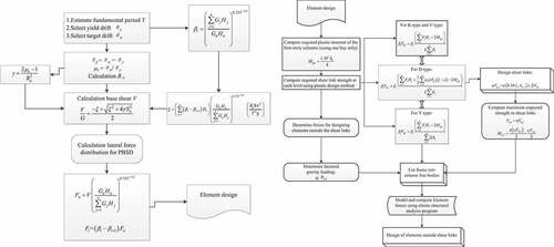
High-strength steel EBFs designed using the PBSD method have similar failure modes and performance objectives; hence, the seismic performance of different types of high-strength steel EBFs tend to be compared. Figure 3 shows the specific design process (Li, Tian, and Liu 2017). The different structures have similar performance objectives, bearing capacity, failure mode, and story drift distribution.

Figure 3. Flowchart of performance-based seismic design method.

2.2. Structural design

Prototype structures were designed on the basis of the performance-based seismic design (PBSD) method. The effects of the story number (5, 10, 15, and 20 stories) and link length (900, 1000, 1100, and 1200 mm) were considered, and 16 structures were designed in total. Figures 4 and 5 show the plane layout and calculation unit of the model. The model number K5-0.9 indicates that the story number is 5, and the link length is 900 mm.

As shown in Figure 4, the bay width is constant in both directions and is equal to 7.2 m. The story height is 3.6 m, there are five bays in the X-direction, three bays in the Y-direction, a braced bay is incorporated along the perimeter of each direction to provide the required lateral resistance, and the shadow part of a single bay frame is taken for analysis and calculation. In the model of EBFs with a high-strength steel, Q345 steel (the nominal yield strength is 345 MPa) is used for the links and braces, and Q460 steel (the nominal yield strength is 460 MPa) is utilized for the frame beams and columns. The elastic modulus is 2.06 × 10⁵ MPa. The buildings are assumed to be located in Xi’an, China, where a peak ground acceleration of 0.3 g with a 10% probability of exceedance over a 50-year period is observed. In addition, a damping of 4% is considered appropriate for a steel building with a structural height not exceeding 50 m, and 3% for structural heights between 50 and 200 m based the requirements of (GB50011-2010 2010).

2.3. Finite element modeling

In this study, the SAP2000 software was used to establish a finite element analysis model. The K-5-0.9 model is taken as an example to specify the performance-based design process, as it is similar to the other models.

K-5-0.9 has a 5-story structure with a total height of 18 m and a total span of 21.6 m. Figure 4 shows the layout of the prototype structure, where the shadow part represents the typical computing units. The links and braces are made of ordinary steel with f_y = 345 MPa, the other components are made of high strength steel with f_y = 460 MPa, and the elastic modulus E is 2.06 × 10⁵ MPa. The link length is 900 mm. Shear yielding links are adopted that use the line element simulation. The two ends of the frame column are defined as P-M hinges, and both ends of the frame beam are defined as bending hinges (M3 hinge). The brace is axially loaded, the middle part is defined as the axial force hinge (P hinge), and the two ends and central part of the links are defined as plastic shear hinges (V2 hinge).

The section of the frame column is a square steel tube, and the section of the other members is a welded H-type steel, as shown in Figure 6, where “H” refers to the welded H-shaped section, with a section depth of h, flange width of b_f, web thickness of t_w, and flange thickness of t_f (in mm). The floor dead load is 5.0 kN/m² (including the deadweight of the floor), the live load is 2.0 kN/m², the roof dead load is 6.0 kN/m², the roof live load is 2.0 kN/m², the snow load is 0.25 kN/m², and the fundamental wind pressure is 0.35 kN/m². The P-delta effect due to the gravity loads of buildings is considered in the SAP2000. The design member sections are listed in Tables A1,A2,A3,A4,A5,A6,a7,A8,A9,A10,A11,A12,A13,A14,A15 and A16 of the Appendix. In the tables, the length ratio of the links is ρ = eV_p/M_p, and the links are shear yielding (or short link) when ρ is <1.6.

Figure 4. Model plan view.

Figure 5. Model elevation.

Figure 6. H-type section.

3. Experimental verification

A 1:2 scaled one-story one-bay K-shaped eccentrically braced high-strength steel frame specimen with a shear link was designed and employed to experimentally study its hysteretic and monotonic performance. The story height and span of the specimen were 1.8 and 3.6 m, respectively. The length of the shear link was 600 mm (ρ = eV_p/M_p = 1.45; where e, V_p, and M_p are the link length, plastic shear capacity, and plastic moment capacity, respectively), ρ = 1.45 < 1.6, and the link was short (or shear yielding) in design.

Beams, columns, and braces were made of steel Q460 with a nominal yield strength of 460 MPa, whereas the link was made of steel Q345 with a nominal yield strength of 345 MPa. Welded joints were used to connect the links to the beams and the other members in the test specimen. Table 1 presents the parameters of the member sections. The member sections are built-up sections, and H-sections are used for the members. Table 2 lists the mechanical properties of the steel. The beam-column joint is a rigid connection, and the link and frame beam are butt welded. Full-depth web stiffeners are provided on both sides of the link web, and the link is provided with intermediate web stiffeners of the transverse type with a spacing of 150 mm and thickness of 10 mm.

Table 1. Member sizes of the specimen.

Member	Section (Chinese designation)
Beam	H225 × 125 × 6 × 10
Column	H150 × 150 × 6 × 10
Brace	H125 × 120 × 6 × 10
Link	H225 × 125 × 6 × 10

Table 2. Mechanical properties of steel.

Steel	Q345B	Q345B	Q460C	Q460C
Thickness t (mm)	6	10	6	10
Yield stress fy (MPa)	427.40	383.33	496.90	468.77
Ultimate strength fu (MPa)	571.10	554.40	658.57	627.97
Yield strain εy(×10^−3)	2.12	1.92	2.39	2.32
Elastic modulus E (×10^5MPa)	2.01	2.00	2.08	2.02
Elongation ratio (%)	26.53	31.01	29.73	35.88

A vertical load of 800 kN is applied to the top of the column by a hydraulic jack to simulate the axial force transferred to the column by the superstructure. The actuator is connected to the reaction wall at one end, and the specimen is connected at the other end to exert a horizontal load. The lateral load is transferred to the frame column on the other side through the loading beam with the hinged connection, causing a synchronous lateral displacement of the frame on the left and right columns, thereby avoiding the influence of the transmission force of the link on the horizontal load transfer (Figure 7). The loading test was monotonically conducted using an actuator at a loading speed of 0.05 mm/s until structural failure. The horizontal reciprocating loading was controlled by a combination of the force and displacement in the pseudo-static test. The specimen was controlled by force before yielding and then by displacements ±Δ_y, ±2Δ_y, ±3Δ_y, ±4Δ_y, ±4.5Δ_y, and ±5.5Δ_y, where Δ_y is the yielding displacement. The specimens were subjected to one cycle per stage before yielding, followed by three displacement cycles until the specimen was destroyed. Figure 8 shows the loading protocol.

Figure 7. Test setup.

Figure 8. Loading protoco.

The SAP2000 finite element (FE) analysis software was used in this study to analyze the performance of the high-strength steel EBFs. An FE model was developed, and the average values of the flange and web plate properties were used as the material properties of each component. The FE models were established using the SAP2000 software (version 15.2.1). In the FE models, the plastic hinges were defined at the column-ends and beam-ends using plastic hinges for the steel columns and beams in the SAP2000 software based on the model presented in Tables 5–6 of FEMA-356 for steel columns and beams. For the shear link, the model presented in Tables 5–6 of FEMA-356 was considered for the nonlinear behavior. The ultimate shear force of the shear link V_u = 1.4V_p based on the experimental results of the shear links. Moreover, the immediate occupancy deformation Δ_IO, life safety plastic deformation Δ_LS, and collapse prevention deformation Δ_CP of the shear link were applied using the parameters suggested by FEMA-356, as shown in Figure 9

Table 3. First three periods of each prototype.

Model ID	K5-0.9	K5-1.0	K5-1.1	K5-1.2
T1	0.656	0.669	0.734	0.763
T2	0.254	0.256	0.279	0.293
T3	0.156	0.156	0.169	0.177
Model ID	K10-0.9	K10-1.0	K10-1.1	K10-1.2
T1	1.064	1.161	1.196	1.214
T2	0.381	0.409	0.425	0.434
T3	0.214	0.229	0.242	0.248
Model ID	K15-0.9	K15-1.0	K15-1.1	K15-1.2
T1	1.648	1.784	1.875	1.951
T2	0.569	0.610	0.641	0.669
T3	0.308	0.331	0.350	0.367
Model ID	K20-0.9	K20-1.0	K20-1.1	K20-1.2
T1	2.180	2.258	2.183	2.412
T2	0.729	0.757	0.682	0.813
T3	0.386	0.403	0.356	0.436
T4	0.283	0.284	0.285	0.299

Table 4. Maximum values of the seismic influence coefficient α_max.

Peak ground acceleration	Peak ground acceleration with a 10% probability of exceedance over 50-year period
	0.05 g	0.10 g	0.15 g	0.20 g	0.30 g	0.40 g
Frequent earthquake	0.04	0.08	0.12	0.16	0.24	0.32
Moderate earthquake	0.12	0.23	0.34	0.45	0.68	0.90
Severe earthquake	0.28	0.50	0.72	0.90	1.20	1.40

Table 5. Design base shear force V_d and displacement Δ_d for each model.

Model ID	K5-0.9	K5-1.0	K5-1.1	K5-1.2
Δd (mm)	23.4219	27.1088	31.8583	34.5970
Vd (kN)	860.8744	860.8744	860.8744	860.8744
Model ID	K10-0.9	K10-1.0	K10-1.1	K10-1.2
Δd (mm)	41.1273	48.6335	51.2053	52.6550
Vd (kN)	1001.4890	1001.4890	1001.4890	1001.4890
Model ID	K15-0.9	K15-1.0	K15-1.1	K15-1.2
Δd (mm)	70.6123	82.9082	91.5186	99.0423
Vd (kN)	1044.2480	1044.2480	1044.2480	1044.2480
Model ID	K20-0.9	K20-1.0	K20-1.1	K20-1.2
Δd (mm)	119.5150	128.4370	123.1033	146.7429
Vd (kN)	1318.1930	1318.1930	1318.1930	1318.1930

Table 6. Yield displacement Δ_y and yield base shear V_y for each model.

Model ID	K5-0.9	K5-1.0	K5-1.1	K5-1.2
Δy (mm)	63.176	63.252	74.837	73.410
Vy (kN)	2322.055	2008.652	2022.252	1826.661
Ke (kN/ mm)	36.755	31.756	27.021	24.882
Model ID	K10-0.9	K10-1.0	K10-1.1	K10-1.2
Δy (mm)	224.301	205.260 Vy	196.960	205.367
Vy (kN)	5461.961	4226.830	3852.211	3906.056
Ke (kN/ mm)	24.350	20.592	19.558	19.0198
Model ID	K15-0.9	K15-1.0	K15-1.1	K15-1.2
Δy (mm)	427.964	445.491	448.235	435.470
Vy (kN)	6328.942	5611.074	5114.461	4591.358
Ke (kN/ mm)	14.788	12.595	11.410	10.543
Model ID	K20-0.9	K20-1.0	K20-1.1	K20-1.2
Δy (mm)	660.905	576.353	544.641	597.594
Vy (kN)	7289.472	5915.312	5832.036	5368.195
Ke (kN/ mm)	11.029	10.263	10.708	8.983

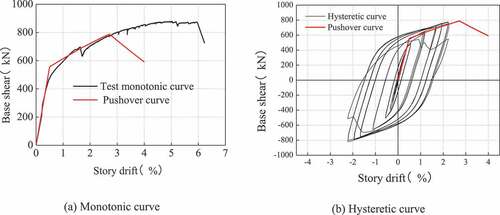
The pushover curve obtained from the pushover analyses of the FE models was compared with the test monotonic loading curves shown in Figure 10. Figure 10 shows the hysteresis curves obtained by cyclic loading. The monotonic curve shows that the K-shaped eccentric brace with a high-strength steel frame exhibits excellent ductility and plastic deformation. The bearing capacity and stiffness of the specimens decrease with increasing plastic deformation of the link. The ultimate bearing capacity of the specimen is approximately 825 kN, and the corresponding ultimate story drift is 3.33%, which exceeds the elastoplastic story drift limit, i.e., 2%. The structure has excellent deformation capacity and ductility, the hysteresis loop is complete and stable, and the EBFs have an excellent energy dissipation capacity. For the test specimen in the elastic state at the beginning of the loading, the hysteretic loop is long and narrow, the specimen only marginally dissipates energy, and the hysteretic circuit gradually opens and tends to be complete when the link in the elastoplastic state.

Figure 9. Generalized force–deformation relationship of a shear link (FEMA-356).

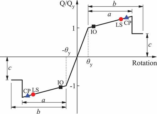
Figure 10. Pushover curves of finite element models.

Figures 11 and 12 show the failure modes of the specimens from the monotonic and hysteretic tests. Figure 13 shows the failure mode of the FE model from the pushover analysis. The failure mode of the FE model is similar to that obtained from the monotonic test. When the frame drift is more significant than H/50 (H is the height of the structure), the deformation of the link reaches the plastic limit state (GB50011-2010 2010), the shear hinge unloads, and the pushover curves exhibit a downward trend. The components in SAP2000 are truss elements, the average values of the material properties of the flanges and web plates were taken as the material model, and the plastic deformation of the structure was concentrated in the plastic hinges by defining the plastic behavior of the plastic hinge reaction structure. When the plastic hinge of the structure reaches the limit state in the FE model, unloading of the hinge occurs, causing the bearing capacity to rapidly decrease. The line element is used for the beams and columns in the FE model. The plastic zone is just a point, and it is different from the actual structure, which is the primary cause of errors.

Figure 11. Failure mode from monotonic test.

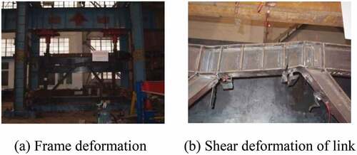
Figure 12. Failure mode from hysteresis test.

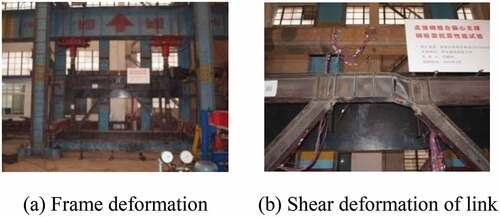
Figure 13. Failure mode of FE model.

4. Pushover analysis

4.1. Fundamental period of the structures

The first three periods of the structure are obtained by modal analysis, as listed in Table 3. Specifically, there is only one period for the SDOF system, while for the multi-degree-freedom system, there is the same number of mode vibrations as the number of degrees of freedom in the model.

The performance curve of the structure is obtained by a pushover analysis using SAP2000 software. The performance curves are transformed into the spectral acceleration–displacement curves (S_ai–S_di curves) of the equivalent SDOF system. Based on the quality participation coefficient α_i corresponding to T_i in each vibration of the structure, the number of vibration modes participating in the combination is determined. The combination of the mass participation ratio should be >0.9, and the capacity spectrum curve corresponding to each period is obtained. This study mainly determines the capacity spectrum curve of the first three periods. The conversion formulae for the capacity spectrum method under period T_i are as follows:

Structural spectral acceleration:

(3) $S_{ai}=\frac{V/G}{{\alpha }_i}$(3)

Structural spectral displacement:

(4) $S_{di}=\frac{\mathrm{\Delta }}{{\gamma }_i{X}_{i,roof}}$(4)

Mass participation ratio:

(5) ${\alpha }_i=\frac{{\left[\sum _{j=1}^N\left(G_j{\phi }_{ji}\right)\right]}^2}{\left[\sum _{j=1}^N{G}_j\right]\left[\sum _{j=1}^N\left(G_j{\phi }_{ji}^2\right)\right]}$(5)

Mode participation ratio:

(6) ${\gamma }_i=\frac{\sum _{j=1}^N\left(G_j{\phi }_{ji}\right)}{\sum _{j=1}^N\left(G_j{\phi }_{ji}^2\right)}$(6)

The representation value of the gravity load

(7) $G=\sum _{j=1}^N{G}_j$(7)

where X_i,roof is the horizontal relative top displacement of the structure under the i-th vibration mode; G_j is the gravity load representation value of the j-story of the structures; $\phi$_ji is the horizontal relative displacement of the j-story under the i-th vibration mode.

4.2. Elastic-to-plastic demand spectrum

The seismic influence coefficient α is specified in the Code for Seismic Design of Buildings (GB50011-2010 2010) of China with the fundamental period T shown in Figure 14.

Figure 14. Seismic influence coefficient α.

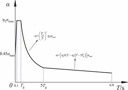
The relationship between the seismic influence coefficient α and the fundamental period T can be expressed as follows:

(8) $\alpha =\left(\frac{{\eta }_2-0.45}{0.1}\right)T{\alpha }_{max}+0.45{\alpha }_{max},0<T\le 0.1\mathrm{s}$(8)

(9) $\alpha ={\eta }_2{\alpha }_{max},0.1<T\le T_{\mathrm{g}}$(9)

(10) $\alpha ={\left(\frac{T_g}{T}\right)}^{\gamma }{\eta }_2{\alpha }_{max},T_{\mathrm{g}}<T\le 5T_{\mathrm{g}}$(10)

(11) $\alpha =\left[{\eta }_2{0.2}^{\gamma }-{\eta }_1\left(T-5T_g\right)\right]{\alpha }_{max},5T_{\mathrm{g}}<T\le 6.0$(11)

where α_max is the maximum value of the seismic influence coefficient, η₂ is the damping adjustment factor, determined by Equation (12)(12) ${\eta }_2=1+\frac{0.05-\zeta }{0.08+1.6\zeta }$(12) , when η₂ < 0.55 and η₂ = 0.55. T_g is the characteristic period, and γ is the attenuation coefficient of the descending curve calculated using Equation (13)(13) $\gamma =0.9+\frac{0.05-\zeta }{0.3+6\zeta }$(13) . η₁ is the adjustment factor for the descent slope of the straight descent part, calculated as follows when η₁ < 0 and η₁ = 0.

(12) ${\eta }_2=1+\frac{0.05-\zeta }{0.08+1.6\zeta }$(12)

where $\zeta$ is the damping ratio of the structure.

(13) $\gamma =0.9+\frac{0.05-\zeta }{0.3+6\zeta }$(13)

(14) ${\eta }_1=0.02+\frac{0.05-\zeta }{4+32\zeta }$(14)

Table 4 presents the maximum value of the seismic influence coefficient.

In the elastic SDOF system, the parameters of the structural demand spectrum curve have the following relationship.

(15) $\alpha =\frac{S_{ae}}{g}=k\beta$(15)

(16) $S_{de}=\frac{M^{\ast }{S}_{ae}}{K}={\left(\frac{T}{4\pi }\right)}^2{S}_{ae}$(16)

where S_ae and S_de are the spectral acceleration and spectral displacement, respectively, k is the peak ground acceleration, β is the dynamic factor, M* is the structural equivalent mass, and K is the stiffness of the structure.

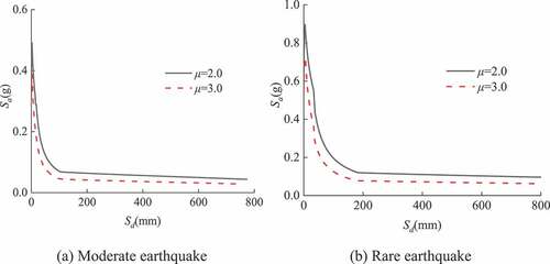
In the elastic-to-plastic SDOF system, the parameters of the structural demand spectrum curve have the following relationship.

(17) $S_a=\frac{S_{ae}}{R_f}=\frac{\alpha g}{R_f}$(17)

(18) $S_d=\frac{\mu }{R_f}{S}_{de}=\frac{\mu }{R_f}{\left(\frac{T}{4\pi }\right)}^2{S}_{ae}=\mu {\left(\frac{T}{4\pi }\right)}^2{S}_a$(18)

where S_a and S_d are the spectral acceleration and spectral displacement in the elastic-to-plastic demand spectrum, respectively, μ is the ductility of the structure; R_f is the strength reduction factor, calculated as follows.

(19) $\begin{array}{c}{R}_f=\left\{\begin{array}{c}1.35{\left(\mu -1\right)}^{0.95}\frac{T}{T_g}+1\\ 1.35{\left(\mu -1\right)}^{0.95}+1\end{array}\right.\\ T\le T_0\\ T>T_0\end{array}$(19)

(20) $T_0=0.75{\mu }^{0.2}{T}_g$(20)

According to Equations (17)(17) $S_a=\frac{S_{ae}}{R_f}=\frac{\alpha g}{R_f}$(17) –(20(20) $T_0=0.75{\mu }^{0.2}{T}_g$(20) ), if the ductility factor of the structure is determined, the elastic-to-plastic demand spectrum curves will be as shown in Figure 15

Figure 15. Elastic-to-plastic demand spectra under different earthquake magnitude.

4.3. Response modification factor R and displacement amplification coefficient C_d

A static pushover analysis was performed using the inverted triangle lateral load distribution specified in the Chinese code (Sun and Ou 2008).

The R and C_d values of the studied frame are determined using the capacity spectrum method. To consider the influence of high-order vibration modes, the performance curve of the structure is transferred to the spectral acceleration–displacement curve (S_ai–S_di curve) of the equivalent SDOF system, and an inelastic demand spectrum of the structure is established. The design base shear V_d and design roof displacement Δ_d of the structure under frequent earthquakes are calculated, as listed in Table 5.

The elastic base shear V_e of the structure is determined on the basis of the seismic performance of the structure under moderate earthquakes. The R and C_d values of the structure can be calculated using Equations (1)(1) $R=\frac{V_e}{V_d}=\frac{V_e}{V_y}\times \frac{V_y}{V_d}=R_{\mu }\times R_{\mathrm{\Omega }}$(1) and (2(2) $C_d=\frac{{\mathrm{\Delta }}_{max}}{{\mathrm{\Delta }}_d}$(2) ).

The capability spectrum method (CSM) is used to calculate the performance coefficient. The solutions to R and C_d based on the CSM are obtained through an iterative process, as shown in Figures 16 and 17.

Figure 16. Capacity spectrum method.

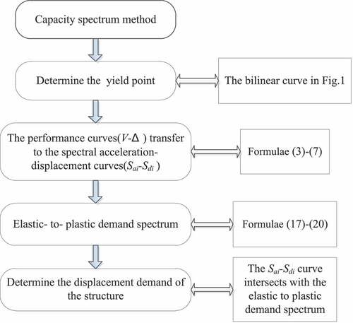
Figure 17. Iteration process.

Taking the K5-0.9 structure as a calculation example, a pushover analysis of K5-0.9 is conducted to obtain the performance curve, and the R and C_d values of the structure are calculated using the CSM.

(1) Determining the yield point of the structure

The performance curve of the structure is transformed into a bilinear line by taking the area enclosed by the curve as unity. The inflection point of the curve is the yield point. Figure 18 shows the sample curve.

Figure 18. Structural performance curve transformed into a bilinear line.

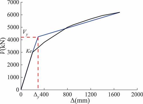
The area enclosed by the pushover curve is equal to that enclosed by the bilinear curve. The significant yield displacement Δ_y and significant yield shear V_y can be obtained from the following formulae:

(21) $A_0=\frac{1}{2}{\mathrm{\Delta }}_y{V}_y+\frac{1}{2}(V_m+V_y)\left({\mathrm{\Delta }}_m-{\mathrm{\Delta }}_y\right)$(21)

(22) ${\mathrm{\Delta }}_y=\frac{V_y}{K_e}=\frac{2A_0-V_m\mathrm{\Delta }}{K_e\mathrm{\Delta }-V_m}$(22)

where A₀ is the area of the pushover curve, Δ_m is the maximum displacement, V_m is the maximum shear, and K_e is the initial stiffness.

The roof displacement and base shear of each model at the yield point are calculated and shown in Table 6.

From Table 6, the significant yield displacement tends to increase as the number of story increases. This is because the lateral stiffness of the structure decreases gradually with an increase in the height of the story, thereby significantly increasing the yield displacement under the same conditions.

The first-order response curve of the model K5-0.9 is plotted by connecting the values of the spectral acceleration and displacement. Figure 19 shows the response curve under each period.

According to the Chinese CSI (2010), the standard value of structures under horizontal seismic action is calculated by the formula:

(23) $F_{ek}={\alpha }_1{G}_{eq}$(23)

where F_ek is the standard value under horizontal seismic action, α₁ is the horizontal seismic influence coefficient, and G_eq is the standard value of the structural gravity load.

The horizontal seismic influence coefficient α₁ and related parameters can be calculated as specified in the Chinese CSI (2010):

${\eta }_2=1+(0.05-\xi )/(0.08+1.6\xi )=1+(0.05-0.04)/(0.08+1.6\times 0.04)=1.06944$

${\alpha }_1={\left(\frac{T_g}{T}\right)}^{\gamma }{\eta }_2{\alpha }_{max}={\left(\frac{0.35}{0.605}\right)}^{0.04}\times 1.06944\times 0.24=0.15525$

$F_{ek}={\alpha }_1{G}_{eq}=0.15525\times 5544.859=860.8744$

where η₂ is the damping adjustment coefficient, ξ is the damping ratio, and α_max is the maximum seismic influence coefficient.

Since Δ_d has a linear relationship with V_d, the ratio value is the initial stiffness K_e, and Δ_d can be obtained as follows:

(24) ${\mathrm{\Delta }}_d=\frac{V_d}{K_e}=\frac{860.8744}{36.7551}=23.4219$(24)

The design base shear force and design roof displacement of each model are calculated. Table 5 lists the results.

(2) Reduction in the seismic demand spectrum

Based on the conditions of site category and earthquake grouping in the design of prototype structures and China’s CSI (2010 version), the numerical relationship between the statistical earthquake period and the seismic influence coefficient can be determined. Figure 15 shows the relationship between the seismic period and the seismic influence coefficient.

Figure 19. Response curve of K5-0.9 model.

4.4. Displacement demand of the structure

The calculated response spectrum curve is intersected with the reduced seismic demand spectrum under moderate and severe earthquake loadings, respectively, and the displacement demand of the structure under different ground motions is obtained by iterating the ductility demand coefficient µ₁.

(1) Response curves intersect the demand spectrum curves under moderate ground motions

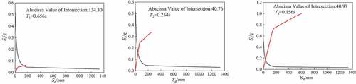
Taking the K5-0.9 model as an example, first, the corresponding acceleration–displacement spectrum curve is obtained under the condition that the ductility demand µ₀ = 2. Second, the demand spectrum curves are intersected with the response spectrum curve of different periods, as shown in Figure 20. Subsequently, the spectral displacements of these intersections are transformed into the roof displacement by applying to Equation (4)(4) $S_{di}=\frac{\mathrm{\Delta }}{{\gamma }_i{X}_{i,roof}}$(4) . The results are: Δ₁ = 248.69 mm, Δ₂ = −29.19 mm, and Δ₃ = 10.65 mm.

A new ductility demand coefficient µ₁ is obtained by taking the square root of the three roof displacements and dividing it by the significant yield displacement Δ_y, as follows:

$\mathrm{\Delta }=\sqrt{{\mathrm{\Delta }}_1^2+{\mathrm{\Delta }}_2^2+{\mathrm{\Delta }}_3^2}=\sqrt{{248.69}^2+{(-29.19)}^2+{10.65}^2}=250.63mm$

${\mu }_1=\frac{2+\mathrm{\Delta }/{\mathrm{\Delta }}_y}{2}=\frac{2+250.63/63.176}{2}=2.98$

The ductility coefficient (µ₁) is used to calculate another demand spectrum. The new roof displacement and ductility demand coefficient (µ₂) are obtained by intersecting the demand spectrum with the response spectrum. Finally, this step is repeated until the two obtained ductility demand coefficients are similar. After repeated calculations, the final iteration results are µ = 2.352 and Δ = 165.221 mm.

(2) Response spectrum curves intersect the demand spectrum curves under severe ground motions

Taking the K5-0.9 model as an example, the corresponding acceleration–displacement spectrum curve is obtained under the condition that the ductility demand µ₀ = 5. The demand spectrum curve is intersected with the response spectrum curve of the first three periods, as shown in Figure 21. The spectral displacements of these intersections are transformed into the roof displacement by applying to Equation (4)(4) $S_{di}=\frac{\mathrm{\Delta }}{{\gamma }_i{X}_{i,roof}}$(4) . The results are: Δ₁ = 356.35 mm, Δ₂ = −39.28 mm, and Δ₃ = 16.45 mm.

$\mathrm{\Delta }=\sqrt{{\mathrm{\Delta }}_1^2+{\mathrm{\Delta }}_2^2+{\mathrm{\Delta }}_3^2}=\sqrt{{356.35}^2+{(-39.28)}^2+{16.45}^2}=358.89mm$

${\mu }_1=\frac{5+\mathrm{\Delta }/{\mathrm{\Delta }}_y}{2}=\frac{2+358.89/63.176}{2}=5.34$

The ductility coefficient (µ₁) is used to calculate another demand spectrum. Another new roof displacement and ductility demand coefficient (µ₂) are computed by intersecting the demand spectrum with the response spectrum. This step is repeated until the two obtained ductility demand coefficients are similar. Through repeated calculations, the final iteration results are µ = 5.347 and Δ = 338.867 mm.

The displacements under moderate earthquake Δ_e and severe earthquake Δ_max of each model are listed in Table 7.

Table 7. Target displacement of each model.

Model ID	K5-0.9	K5-1.0	K5-1.1	K5-1.2
Δe (mm)	165.221	186.075	211.283	221.144
Δmax (mm)	338.867	320.172	370.194	395.292
Model ID	K10-0.9	K10-1.0	K10-1.1	K10-1.2
Δe (mm)	422.989	444.456	462.236	467.041
Δmax (mm)	631.079	769.384	832.512	838.260
Model ID	K15-0.9	K15-1.0	K15-1.1	K15-1.2
Δe (mm)	816.794	913.236	1014.637	1108.075
Δmax (mm)	1080.138	1212.358	1356.607	1312.717
Model ID	K20-0.9	K20-1.0	K20-1.1	K20-1.2
Δe (mm)	1249.801	1248.789	1249.081	1248.882
Δmax (mm)	1640.751	1660.204	1662.825	1753.763

The response curve shows that V_e and Δ_e have a linear relationship, and the proportion coefficient is the initial stiffness K_e. Therefore, the shear force V_e in elasticity can be calculated.

$V_e=K_e{\mathrm{\Delta }}_e=36.7551\times 165.221=6072.747kN$

Table 8 presents the base shear force of each model.

Table 8. Base shear force V_e of each model.

Model ID	K5-0.9	K5-1.0	K5-1.1	K5-1.2
Ve (kN)	6072.747	5909.027	5709.287	5502.714
Model ID	K10-0.9	K10-1.0	K10-1.1	K10-1.2
Ve (kN)	10,300.192	8710.431	8272.951	8045.177
Model ID	K15-0.9	K15-1.0	K15-1.1	K15-1.2
Ve (kN)	12,079.136	11,502.423	11,577.241	11,682.932
Model ID	K20-0.9	K20-1.0	K20-1.1	K20-1.2
Ve (kN)	13,784.725	12,816.761	13,375.252	11,218.731

Finally, the response modification factor R and displacement amplification factor C_d of K5-0.9 are calculated.

$R=\frac{V_e}{V_d}=\frac{6072.747}{860.8744}=7.054$

$C_d=\frac{{\mathrm{\Delta }}_{max}}{{\mathrm{\Delta }}_d}=\frac{338.867}{23.4219}=14.468$

The response modification factor R and displacement amplification factor C_d of the other models are shown in Table 9.

Table 9. Response modification factor R and displacement amplification factor C_d of each model.

Model ID	K5-0.9	K5-1.0	K5-1.1	K5-1.2
R	7.054	6.864	6.632	6.392
Cd	14.468	11.812	11.620	11.425
Model ID	K10-0.9	K10-1.0	K10-1.1	K10-1.2
R	10.285	8.697	8.260	8.033
Cd	15.344	15.820	16.258	15.920
Model ID	K15-0.9	K15-1.0	K15-1.1	K15-1.2
R	11.567	11.015	11.087	11.188
Cd	15.297	14.623	14.823	13.254
Model ID	K20-0.9	K20-1.0	K20-1.1	K20-1.2
R	10.457	9.723	10.147	8.511
Cd	13.728	12.926	13.508	11.951

From Table 9, the minimum and maximum values of the response modification factor R calculated using the pushover method are 6.392 and 11.567, respectively. The minimum and maximum values of the displacement amplification factor C_d calculated using the pushover method are 11.620 and 16.258, respectively. The two factors are significantly higher than 0.25 and 2.8125 specified in China’s CSI (2010 Edition).

Figure 20. Intersection of the K5-0.9 demand spectrum with the response curve under moderate ground motions.

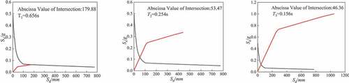
Figure 21. Intersection of the K5-0.9 demand spectrum with the response curve under severe ground motions.

4.5. Effect of number of stories and length of link

In the simulation, the number of stories and link length are used as the parameters. The influence of the two parameters on the two factors is explained below.

(1) Response modification factor R

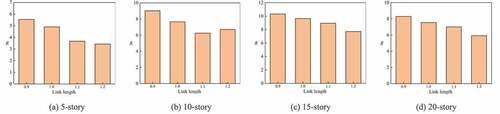
Figure 22 shows the influence of the change in the total number of stories on the R value. In addition to the 20-story, the value of the response modification factor R increases as the number of stories increases.

Figure 23 illustrates the influence of the link length on the R value. The response modification factor R of the 5-story and 10-story models decreases as the length of the link increases. The changing orderliness of R on the 15-and 20-story models is not evident.

Figure 22. Effect of the number of stories on the R value.

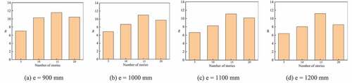
Figure 23. Effect of the link length on the R value.

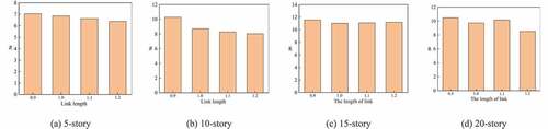
(2) Displacement amplification factor C_d

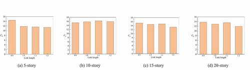
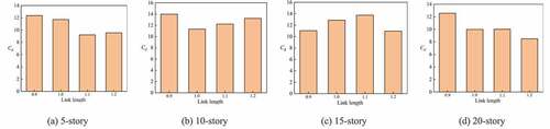
Figure 24 shows the influence of the total number of stories on the C_d value. The number of stories has little influence on the value of the displacement amplification factor C_d.

Figure 25 illustrates the influence of the link length on the C_d value. With the exception of the 10-story, the displacement amplification factor C_d of the other stories decreases as the length of link increases, but is not distinct.

Figure 24. Effect of the number of stories on the C_d value.

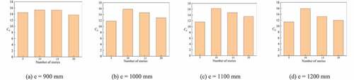
Figure 25. Effect of the link length on the C_d value.

5. Calculation of response modification factor and displacement amplification factor based on increment dynamic analysis

5.1. Selection of ground motions

Nine natural ground motions with an average fluctuation of no more than 20% and ground motions in the ranges of 0.1− T_g and 0.2T₁ − 1.5T₁ are selected. The artificial ground motion is simulated using Seismosignal. These 10 ground motions are used for the analysis (Table 10 details each ground motion). The average ground motion curve of the 10 groups is obtained and placed in the same coordinate axis, as shown in Figure 26. It is checked whether the selected ground motions meet the aforementioned requirements.

Figure 26. Response spectra of seismic records.

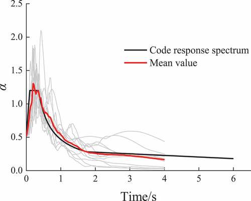
Table 10. Seismic ground motion records.

No.	Earthquake number	Earthquake event	Station	M	R/km	PGA/g	PGV/(cm/s)
1	NGA0181	Imperial Valley 1979/10/15 23:16	942 El Centro Array #6	5	1.0	0.439	109.8
2	NGA0829	Cape Mendocino 1992/04/25 18:06	89,324 Rio Dell Overpass – FF	7.0	14.3	0.549	42.1
3	NGA0292	Irpinia, Italy 1980/11/23 19:34	Sturno	6.5	3.2	0.358	52.7
4	NGA0727	Superstitn Hills(B) 1987/11/24 13:16	01335 El Centro Imp. Co. Cent	6.5	5.6	0.894	42.2
5	NGA0802	Loma Prieta 1989/10/18 00:05	58,065 Saratoga – Aloha Ave	6.9	13.0	0.324	41.2
6	NGA0821	Erzincan, Turkey 1992/03/13	95 Erzincan	6.9	2.0	0.496	64.3
7	NGA1485	Chi-Chi, Taiwan 1999/09/20	TCU045	7.6	24.1	0.512	39.0
8	NGA0068	San Fernando 1971/02/09 14:00	135 LA – Hollywood Stor Lot	6.6	21.2	0.210	18.9
9	NGA0960	Northridge 1994/01/17 12:31	90,057 Canyon Country – W Lost Cany	6.7	13.0	0.482	45.1
10	NGA1605	Duzce, Turkey 1999/11/12	Duzce	7.1	8.2	0.535	83.5

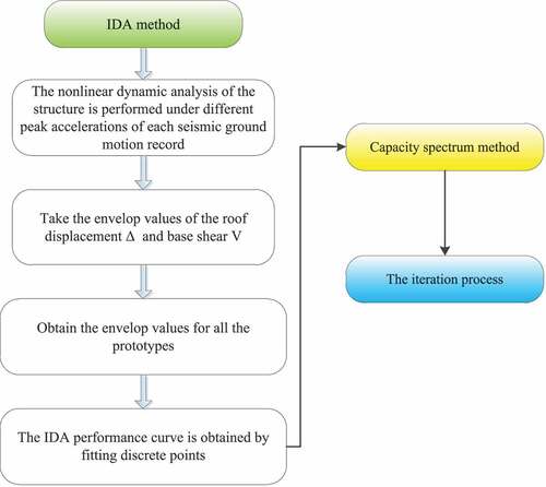
5.2. Steps of IDA

In this study, the increment dynamic analysis (IDA) of several ground motion records was adopted for each structure. The basic process is illustrated as follows:

1. Use SAP2000 to establish the FE model of the structures

2. Select appropriate ground motions according to relevant specifications

3. Amplify each ground motion to prepare a group of ground motions, including mild, moderate, and severe earthquakes

4. Implement the inelastic dynamic time-history analysis using each group of amplified ground motions

5. Extract the values of the base shear and roof displacement and plot the envelope curve (V–Δ) obtained from each group of ground motions in the same coordinate system. The response curve of the structure is then obtained by curve fitting.

5.3. Calculation of Factors by IDA

The specific steps in obtaining the factors via the CSM are illustrated as follows:

1. A nonlinear dynamic analysis is conducted under a group of different ground motions. The envelope curve of the roof displacement and bottom shear force is plotted. All the curves can be obtained via the other ground motion groups.

2. Fit all the obtained Δ–V envelope curves to compute the response curve of the IDA. This curve is similar to the pushover curve.

3. The yield shear force V_y and yield displacement Δ_y are determined by making the fitted IDA response curve bilinear.

4. Transform the fitted IDA response curve into spectrum acceleration–displacement curve (S_ai–S_di)

5. Plot the response curve obtained in step 4 and the elastic-to-plastic demand spectrum of the different ground motions in the same coordinate system, and determine the capacity point of the different ground motions through iteration.

6. Use Equations (1)(1) $R=\frac{V_e}{V_d}=\frac{V_e}{V_y}\times \frac{V_y}{V_d}=R_{\mu }\times R_{\mathrm{\Omega }}$(1) and (2(2) $C_d=\frac{{\mathrm{\Delta }}_{max}}{{\mathrm{\Delta }}_d}$(2) ) to calculate the response modification factor R and displacement amplification factor C_d of the structure.

The steps are shown in the Figure 27.

Figure 27. Steps involved in the increment dynamic analysis.

5.4. Response curve of IDA

The base shear–displacement curve of K5-0.9 is obtained by fitting all the bottom shear and displacement under different ground motions, as shown in Figure 28. The base shear–displacement curve obtained by the IDA is similar to that obtained by the pushover analysis. The curve is transformed into a bilinear curve to obtain a significant yield point. The fitted curves of the other structural models are calculated by analogy (Table 11).

Figure 28. Fitted response curve of K5-0.9 model.

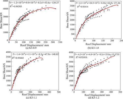
Table 11. Significant yield displacement Δ_y and significant yield shear force V_y for each model.

Model ID	K5-0.9	K5-1.0	K5-1.1	K5-1.2
Δy (mm)	60.967	60.017	70.234	73.061
Vy (kN)	2195.842	1892.427	1620.401	1559.146
K0 (kN/ mm)	36.016	31.531	23.071	21.340
Model ID	K10-0.9	K10-1.0	K10-1.1	K10-1.2
Δy (mm)	211.621	193.394	183.535	170.478
Vy (kN)	5356.745	4151.243	3219.526	3205.898
K0 (kN/ mm)	25.312	21.465	17.541	18.805
Model ID	K15-0.9	K15-1.0	K15-1.1	K15-1.2
Δy (mm)	379.506	402.104	416.743	408.640
Vy (kN)	5932.309	5145.951	4607.700	4093.967
K0 (kN/ mm)	15.631	12.797	11.056	10.018
Model ID	K20-0.9	K20-1.0	K20-1.1	K20-1.2
Δy (mm)	581.778	507.546	468.513	508.515
Vy (kN)	6512.798	5185.966	4901.841	4158.447
K0 (kN/ mm)	11.194	10.217	10.462	8.177

5.5. Calculation of response modification factor and displacement amplification factor

First, each ground motion is dispersed into a series of ground motion data with different intensities using the amplified coefficient. The base shear–displacement curve can be obtained using the dynamic time-history analysis with the ground motions. The curve is then transformed into the response spectrum curve of the IDA by applying to the CSM and intersected with the demand spectrum under moderate and severe earthquakes. The maximum displacement Δ_max under severe earthquake and moderate earthquake Δ_e are calculated considering a high-order vibration mode. The results are summarized in Table 12.

Table 12. Target displacement of each prototype.

Model ID	K5-0.9	K5-1.0	K5-1.1	K5-1.2
Δe	132.619	133.931	137.108	138.562
Δmax	295.526	320.172	344.020	385.670
Model ID	K10-0.9	K10-1.0	K10-1.1	K10-1.2
Δe	357.217	361.577	412.210	398.388
Δmax	553.160	529.122	698.235	705.203
Model ID	K15-0.9	K15-1.0	K15-1.1	K15-1.2
Δe	689.387	787.021	845.701	804.216
Δmax	737.691	1049.963	1298.993	1142.618
Model ID	K20-0.9	K20-1.0	K20-1.1	K20-1.2
Δe	977.525	972.903	883.227	955.507
Δmax	1481.195	1288.580	1262.487	1371.208

Finally, the R and C_d values of each model are calculated using the method described in the previous section. Table 13 lists the ultimate results.

Table 13. Response modification factor R and displacement amplification factor C_d of each model.

Model ID	K5-0.9	K5-1.0	K5-1.1	K5-1.2
R	5.548	4.905	3.674	3.435
Cd	12.364	11.726	9.219	9.560
Model ID	K10-0.9	K10-1.0	K10-1.1	K10-1.2
R	9.028	7.656	6.256	6.707
Cd	13.981	11.340	12.230	13.241
Model ID	K15-0.9	K15-1.0	K15-1.1	K15-1.2
R	10.319	9.645	8.954	7.715
Cd	11.042	12.867	13.753	10.962
Model ID	K20-0.9	K20-1.0	K20-1.1	K20-1.2
R	8.301	7.541	7.010	5.927
Cd	12.578	9.988	10.020	8.506

The minimum and maximum values of R calculated using the IDA are 3.435 and 10.319, respectively. The minimum and maximum values of the displacement amplification factor C_d are 8.506 and 13.981, respectively.

5.6. Effects of story height and link length

The story height and link length are used as the changed parameters to demonstrate their influence on the factors.

(1) Response modification factor R

Figure 29 shows the influence of the total number of stories on the R value. In addition to the 20-story model, the structural response modification factor R increases as the number of stories increase.

Figure 30 illustrates the influence of the link length on the R value. R decreases gradually as the link length increases.

Figure 29. Effect of the number of stories on the R value.

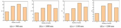
Figure 30. Effect of the link length on the R value.

(2) Displacement amplification factor C_d

Figure 31 shows the influence of the total number of stories on the C_d value. The number of stories has little effect on the value of the displacement amplification factor C_d.

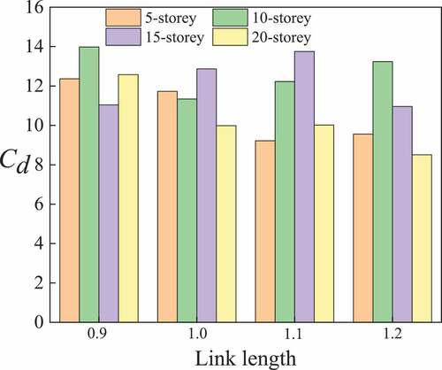
Figure 32 illustrates the influence of the link length on the C_d value. The displacement amplification factor C_d for the 5-story and 20-story models decreases as the link length increases. However, the changing orderliness of C_d for the 10-story and 15-story models is not evident.

Figure 31. Effect of the number of stories on the C_d value.

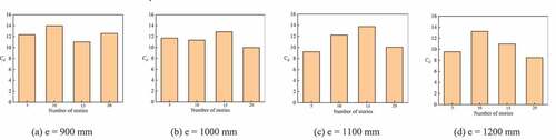
Figure 32. Effect of the link length on the C_d value.

6. Recommended values of R and C_d

A pushover analysis is a static elastoplastic analysis method. A certain lateral force distribution model is used to simulate horizontal earthquake action. It is an approximate calculation method that can help simulate the response of structures under earthquake motion. However, the IDA is used to input seismic ground motions to the structure. The response of a structure is real under earthquakes, and the IDA approach has its drawbacks in that the results are relatively discrete. The R and C_d values are influenced by the IDA curves and fitting data. Therefore, this study adopts two methods to analyze the response modification factor.

The results obtained by the pushover analysis and IDA are compared in terms of the story height and link length. The response modification factor and displacement amplification factor are summarized in Tables 14 and 15, respectively.

Table 14. Summary of response modification factor R of each model.

Model ID	K5-0.9	K5-1.0	K5-1.1	K5-1.2
Pushover	7.054	6.864	6.632	6.392
IDA	5.548	4.905	3.674	3.435
Model ID	K10-0.9	K10-1.0	K10-1.1	K10-1.2
Pushover	10.285	8.697	8.260	8.033
IDA	9.028	7.656	6.256	6.707
Model ID	K15-0.9	K15-1.0	K15-1.1	K15-1.2
Pushover	11.567	11.015	11.087	11.188
IDA	10.319	9.645	8.954	7.715
Model ID	K20-0.9	K20-1.0	K20-1.1	K20-1.2
Pushover	10.457	9.723	10.147	8.511
IDA	8.301	7.541	7.010	5.927

Table 15. Summary of displacement amplification factor C_d of each model.

Model ID	K5-0.9	K5-1.0	K5-1.1	K5-1.2
Pushover	14.468	11.812	11.620	11.425
IDA	12.364	11.726	9.219	9.560
Model ID	K10-0.9	K10-1.0	K10-1.1	K10-1.2
Pushover	15.344	15.820	16.258	15.920
IDA	13.981	11.340	12.230	13.241
Model ID	K15-0.9	K15-1.0	K15-1.1	K15-1.2
Pushover	15.297	14.623	14.823	13.254
IDA	11.042	12.867	13.753	10.962
Model ID	K20-0.9	K20-1.0	K20-1.1	K20-1.2
Pushover	13.728	12.926	13.508	11.951
IDA	12.578	9.988	10.020	8.506

Clearly, the values of the response modification factor R and displacement amplification factor C_d calculated by the pushover method are higher than those computed using the IDA, and the maximum difference in the response modification factor is 25.9%. However, the statistical regularity of the displacement amplification factor is unclear. This is because in the calculation and simulation, the dispersion in the displacement amplification factor calculated by the IDA is significant. The maximum difference in the displacement amplification factor C_d is 38.5%.

The values of the response modification factor and displacement amplification factor are averaged and then associated with the structural ductility coefficient µ_s and the structural period T, respectively. Figures 33–35 show the R–µ_s, R–T, and C_d–T curves by fitting.

Figure 33. Relationship between response modification factor R and ductility demand µ_s.

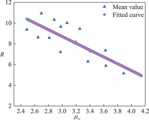
Figure 33 shows the fitted curve between R and ductility coefficient µ_s. From the curve, the relationship can be defined as R = −3.286 µ_s+18.568.

Figure 34 shows the fitted curves between R and period T for the 5-, 10-, and 15-story structures. From the curves, the relationship R = 4.275T₁ + 4.127 can be obtained. However, there is no evident relationship between R and period T for the 20-story structure. The recommended value is R = 7.194.

Figure 35 shows the fitted curves of C_d for the 10-, 15-, and 20-story structures. The relationship can be defined as C_d = −2.525T₁ + 18.645. However, there is no evident relationship between C_d and period T for the 5-story structure. The recommended value is C_d = 12.33.

The calculation formula for the response modification factor R associated with the structural period T is applicable to 5–15 story structures, not to the 20-story one. This is because the deformation in the 20-story structure is different from that in the other structures. The deformation response of high-rise buildings is dominated by bending deformation underground motions, whereas mid- and low-rise buildings are dominated by shear deformation. In the simulation, it is assumed that all the models exhibit shear deformation.

On the other hand, the calculation formula for C_d associated with the structural period T is suitable for 10–20 story structures, not for the 20-story structure. This is because the data of the 5-story model are discrete in the simulation calculation; therefore, the relationship is not evident. However, the statistical regularity between the average values of the response modification factor R and ductility demand µ is evident, which follows a linear distribution, whereas the statistical regularity between the displacement amplification factor C_d and ductility demand is unclear. This is because in the simulation, the dispersion in the displacement amplification factor calculated by the IDA is strong, and the maximum difference in the displacement amplification factor C_d is 38.5%.

The response modification factor R and displacement amplification factor C_d are summarized. Figure 36 and 37 show the regularity between the total number of stories and structural factors.

Figure 36 compares all the R values calculated by the pushover analysis. The values of the 5-, 10-, 15-, and 20-story models range from 6.392 to 7.054, 8.033 to 10.285, 11.015 to 11.567, and 8.511 to 10.457, respectively. Furthermore, when the number of stories is the same, the value of R has little difference, and the overall fluctuation is not evident.

Figure 37 shows all the C_d values calculated by the IDA. It can be concluded that the values of the 5-, 10-, 15-, and 20-story models range from 9.219 to 12.364, 11.340 to 13.981, 10.962 to 13.753, and 8.506 to 12.578, respectively. The values of C_d in the same story do not fluctuate much. Moreover, the displacement amplification coefficient C_d tends to decrease as the length of the link increases, and there is no significant relationship between C_d and the number of stories. The overall fluctuation is not remarkable.

Figure 34. Fitted curve of response modification factor.

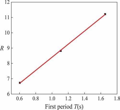
Figure 35. Fitted curve of displacement amplification factor.

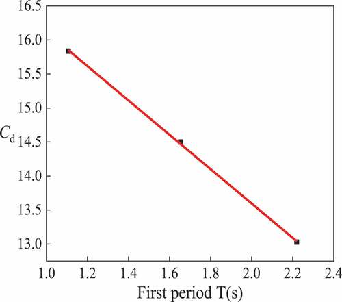
Figure 36. Influence of the number of stories on R value.

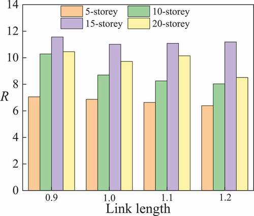
Figure 37. Influence of the number of stories on C_d value.

7. Conclusions

This study compared the calculation results of the pushover analysis and IDA and demonstrated the changing regularity between the factors and the number of stories and link length. Relevant R and C_d formulae in terms of the ductility demand and structural period were obtained. Finally, appropriate values of R and C_d were recommended. The results of the study can be summarized as follows:

(1) The response modification factor R and displacement amplification factor C_d of K-shaped eccentrically braced high-strength steel frame are closely related to the story height and link length. Based on the pushover analysis and IDA, the response modification factor R increases with an increase in the total number of stories, except for the 20-story structure.

(2) The response modification factor R is 2.8125 greater than the value specified in the seismic code of China. This demonstrates that the code does not make full use of the structural ductility, which is not economical and reasonable for seismic design.

(3) Through the analysis, the average R value obtained using the two analysis methods is taken as 7.194 for the 20-story structure. The relationship between the response modification factor R and the first period T₁ of structures with less than 20 stories is linear, R = 4.275T₁ + 4.1274. The relationship between the response modification factor R and ductility coefficient µ_s can be defined as R = −3.286 µ_s+18.568.

(4) There is a linear relationship between the displacement amplification factor C_d and the first period T₁ of structures with 5 stories or more, and it can be defined as C_d = −2.525T₁ + 18.645. While there is no evident relationship between the displacement amplification factor C_d and the period T₁ for the 5-story structure. The recommended value can be taken as C_d = 12.331.

Disclosure statement

No potential conflict of interest was reported by the authors.

Additional information

Funding

The authors are grateful for the financial support received from the Project Supported by Natural Science Basic Research Plan in Shaanxi Province of China [Program No. 2021JM-330, 2021JM-333] and The Project Supported by Shaanxi Postdoctoral Science Foundation [No. 2018BSHEDZZ24].

Appendix

Table A1. K5-0.9 sections.

Story	Frame beam	Frame column	Brace	link	$\rho =\frac{e}{(M_P/V_P)}$
5	H320 × 140 × 6 × 12	□300 × 300 × 12 × 12	H200 × 200 × 8 × 12	H320 × 140 × 6 × 12	1.43
4	H360 × 160 × 10 × 16	□300 × 300 × 12 × 12	H220 × 220 × 8 × 12	H410 × 160 × 8 × 14	1.35
3	H400 × 180 × 10 × 16	□350 × 350 × 12 × 12	H240 × 240 × 8 × 12	H430 × 180 × 10 × 16	1.31
2	H450 × 180 × 10 × 16	□400 × 400 × 12 × 12	H260 × 260 × 10 × 16	H490 × 180 × 10 × 16	1.27
1	H470 × 180 × 8 × 12	□400 × 400 × 12 × 12	H260 × 260 × 10 × 16	H520 × 180 × 10 × 16	1.24

Table A2. K5-1.0 sections.

Story	Frame beam	Frame column	Brace	link	$\rho =\frac{e}{(M_P/V_P)}$
5	H320 × 140 × 6 × 12	□300 × 300 × 12 × 12	H200 × 200 × 8 × 12	H300 × 150 × 6 × 12	1.52
4	H330 × 150 × 10 × 16	□300 × 300 × 12 × 12	H220 × 220 × 8 × 12	H460 × 200 × 6 × 12	1.12
3	H370 × 180 × 10 × 16	□350 × 350 × 12 × 12	H240 × 240 × 8 × 12	H460 × 200 × 8 × 14	1.24
2	H400 × 180 × 10 × 16	□400 × 400 × 12 × 12	H260 × 260 × 10 × 16	H430 × 200 × 10 × 16	1.34
1	H430 × 180 × 10 × 16	□400 × 400 × 12 × 12	H260 × 260 × 10 × 16	H460 × 200 × 10 × 16	1.32

Table A3. K5-1.1 sections.

Story	Frame beam	Frame column	Brace	link	$\rho =\frac{e}{(M_P/V_P)}$
5	H320 × 120 × 6 × 10	□300 × 300 × 12 × 12	H200 × 200 × 8 × 12	H300 × 150 × 5 × 12	1.43
4	H390 × 180 × 6 × 10	□300 × 300 × 12 × 12	H220 × 220 × 8 × 12	H420 × 200 × 6 × 12	1.25
3	H370 × 180 × 8 × 14	□350 × 350 × 12 × 12	H240 × 240 × 8 × 12	H410 × 200 × 8 × 14	1.39
2	H410 × 180 × 8 × 14	□400 × 400 × 12 × 12	H240 × 240 × 8 × 12	H390 × 200 × 10 × 16	1.51
1	H430 × 180 × 8 × 14	□400 × 400 × 12 × 12	H240 × 240 × 8 × 12	H410 × 200 × 10 × 16	1.49

Table A4. K5-1.2 sections.

Story	Frame beam	Frame column	Brace	link	$\rho =\frac{e}{(M_P/V_P)}$
5	H300 × 120 × 6 × 10	□300 × 300 × 12 × 12	H200 × 200 × 8 × 12	H300 × 150 × 5 × 12	1.57
4	H350 × 150 × 6 × 12	□300 × 300 × 12 × 12	H220 × 220 × 8 × 12	H380 × 180 × 6 × 12	1.51
3	H380 × 150 × 8 × 14	□350 × 350 × 12 × 12	H240 × 240 × 8 × 12	H380 × 220 × 8 × 14	1.43
2	H420 × 150 × 8 × 14	□400 × 400 × 12 × 12	H240 × 240 × 8 × 12	H430 × 220 × 8 × 14	1.40
1	H440 × 150 × 8 × 14	□400 × 400 × 12 × 12	H240 × 240 × 8 × 12	H450 × 220 × 8 × 14	1.38

Table A5. K10-0.9 sections.

Story	Frame beam	Frame column	Brace	link	$\rho =\frac{e}{(M_P/V_P)}$
10	H300 × 150 × 8 × 14	□350 × 350 × 12 × 12	H220 × 220 × 10 × 16	H300 × 150 × 8 × 14	1.52
9	H370 × 150 × 10 × 16	□350 × 350 × 12 × 12	H220 × 220 × 10 × 16	H370 × 150 × 10 × 16	1.55
8	H490 × 180 × 10 × 16	□400 × 400 × 16 × 16	H240 × 240 × 12 × 18	H490 × 180 × 10 × 16	1.27
7	H500 × 200 × 12 × 18	□400 × 400 × 16 × 16	H240 × 240 × 12 × 18	H500 × 200 × 12 × 18	1.22
6	H570 × 200 × 12 × 18	□450 × 450 × 20 × 20	H260 × 260 × 12 × 18	H570 × 200 × 12 × 18	1.18
5	H540 × 240 × 14 × 20	□450 × 450 × 20 × 20	H280 × 280 × 12 × 18	H540 × 240 × 14 × 20	1.08
4	H580 × 240 × 14 × 20	□500 × 500 × 20 × 20	H280 × 280 × 12 × 18	H580 × 240 × 14 × 20	1.06
3	H610 × 240 × 14 × 20	□500 × 500 × 20 × 20	H280 × 280 × 12 × 18	H610 × 240 × 14 × 20	1.05
2	H630 × 240 × 14 × 20	□580 × 580 × 25 × 25	H280 × 280 × 12 × 18	H630 × 240 × 14 × 20	1.04
1	H640 × 240 × 14 × 20	□580 × 580 × 25 × 25	H280 × 280 × 12 × 18	H640 × 240 × 14 × 20	1.04

Table A6. K10-1.0 sections.

Story	Frame beam	Frame column	Brace	Link	$\rho =\frac{e}{(M_P/V_P)}$
10	H330 × 150 × 6 × 12	□300 × 300 × 12 × 12	H200 × 200 × 10 × 16	H340 × 160 × 6 × 12	1.41
9	H420 × 200 × 6 × 12	□350 × 350 × 12 × 12	H200 × 200 × 10 × 16	H420 × 200 × 8 × 14	1.26
8	H400 × 200 × 10 × 16	□350 × 350 × 16 × 16	H240 × 240 × 10 × 16	H450 × 200 × 10 × 16	1.33
7	H460 × 200 × 10 × 16	□350 × 350 × 16 × 16	H240 × 240 × 10 × 16	H530 × 250 × 10 × 16	1.08
6	H480 × 220 × 10 × 16	□400 × 400 × 20 × 20	H260 × 260 × 12 × 18	H500 × 200 × 12 × 18	1.36
5	H520 × 200 × 10 × 16	□400 × 400 × 20 × 20	H260 × 260 × 12 × 18	H550 × 240 × 12 × 18	1.36
4	H490 × 220 × 12 × 18	□500 × 500 × 20 × 20	H260 × 260 × 12 × 18	H580 × 250 × 12 × 18	1.11
3	H510 × 220 × 12 × 18	□500 × 500 × 20 × 20	H260 × 260 × 12 × 18	H610 × 250 × 12 × 18	1.09
2	H520 × 220 × 12 × 18	□590 × 590 × 22 × 22	H260 × 260 × 12 × 18	H630 × 250 × 12 × 18	1.08
1	H530 × 220 × 12 × 18	□590 × 590 × 22 × 22	H260 × 260 × 12 × 18	H640 × 250 × 12 × 18	1.08

Table A7. K10-1.1 sections.

Story	Frame beam	Frame column	Brace	Link	$\rho =\frac{e}{(M_P/V_P)}$
10	H300 × 150 × 6 × 12	□300 × 300 × 12 × 12	H200 × 200 × 10 × 16	H310 × 180 × 6 × 12	1.43
9	H450 × 150 × 6 × 12	□350 × 350 × 12 × 12	H200 × 200 × 10 × 16	H380 × 180 × 8 × 14	1.54
8	H410 × 200 × 8 × 14	□400 × 400 × 16 × 16	H240 × 240 × 10 × 16	H490 × 220 × 10 × 16	1.33
7	H470 × 200 × 8 × 14	□400 × 400 × 16 × 16	H240 × 240 × 10 × 16	H470 × 220 × 10 × 16	1.34
6	H440 × 220 × 10 × 16	□450 × 450 × 20 × 20	H260 × 260 × 10 × 16	H530 × 250 × 10 × 16	1.19
5	H470 × 220 × 10 × 16	□450 × 450 × 20 × 20	H260 × 260 × 10 × 16	H580 × 250 × 10 × 16	1.16
4	H500 × 220 × 10 × 16	□500 × 500 × 20 × 20	H260 × 260 × 10 × 16	H530 × 250 × 12 × 18	1.25
3	H520 × 220 × 10 × 16	□500 × 500 × 20 × 20	H260 × 260 × 10 × 16	H550 × 250 × 12 × 18	1.23
2	H530 × 220 × 10 × 16	□580 × 580 × 25 × 25	H260 × 260 × 12 × 18	H570 × 250 × 12 × 18	1.22
1	H540 × 220 × 10 × 16	□580 × 580 × 25 × 25	H260 × 260 × 12 × 18	H570 × 250 × 12 × 18	1.22

Table A8. K10-1.2 sections.

Story	Frame beam	Frame column	Brace	Link	$\rho =\frac{e}{(M_P/V_P)}$
10	H300 × 150 × 6 × 12	□300 × 300 × 12 × 12	H200 × 200 × 10 × 16	H310 × 180 × 6 × 12	1.56
9	H450 × 150 × 6 × 12	□350 × 350 × 12 × 12	H200 × 200 × 10 × 16	H380 × 180 × 8 × 14	1.67
8	H410 × 200 × 8 × 14	□400 × 400 × 16 × 16	H240 × 240 × 10 × 16	H490 × 220 × 10 × 16	1.45
7	H470 × 200 × 8 × 14	□400 × 400 × 16 × 16	H240 × 240 × 10 × 16	H470 × 220 × 10 × 16	1.47
6	H440 × 220 × 10 × 16	□450 × 450 × 20 × 20	H260 × 260 × 10 × 16	H530 × 250 × 10 × 16	1.30
5	H470 × 220 × 10 × 16	□450 × 450 × 20 × 20	H260 × 260 × 10 × 16	H580 × 250 × 10 × 16	1.27
4	H500 × 220 × 10 × 16	□500 × 500 × 20 × 20	H260 × 260 × 10 × 16	H530 × 250 × 12 × 18	1.36
3	H520 × 220 × 10 × 16	□500 × 500 × 20 × 20	H260 × 260 × 10 × 16	H550 × 250 × 12 × 18	1.35
2	H530 × 220 × 10 × 16	□580 × 580 × 25 × 25	H260 × 260 × 12 × 18	H570 × 250 × 12 × 18	1.34
1	H540 × 220 × 10 × 16	□580 × 580 × 25 × 25	H260 × 260 × 12 × 18	H570 × 250 × 12 × 18	1.34

Table A9. K15-0.9 sections.

Story	Frame beam	Frame column	Brace	Link	$\rho =\frac{e}{(M_P/V_P)}$
15	H330 × 150 × 8 × 14	□250 × 250 × 10 × 10	H200 × 200 × 10 × 16	H370 × 180 × 6 × 12	1.14
14	H410 × 200 × 8 × 14	□300 × 300 × 12 × 12	H220 × 220 × 10 × 16	H370 × 180 × 10 × 16	1.35
13	H450 × 200 × 10 × 16	□300 × 300 × 12 × 12	H240 × 240 × 10 × 16	H470 × 200 × 10 × 16	1.18
12	H510 × 200 × 10 × 16	□350 × 350 × 16 × 16	H260 × 260 × 10 × 16	H560 × 240 × 10 × 16	0.99
11	H520 × 200 × 12 × 18	□400 × 400 × 16 × 16	H260 × 260 × 10 × 16	H540 × 240 × 12 × 18	1.05
10	H530 × 220 × 12 × 18	□450 × 450 × 18 × 18	H280 × 280 × 12 × 18	H590 × 240 × 18 × 20	1.26
9	H560 × 220 × 12 × 18	□500 × 500 × 20 × 20	H280 × 280 × 12 × 18	H560 × 240 × 14 × 20	1.07
8	H520 × 240 × 14 × 20	□550 × 550 × 20 × 20	H300 × 300 × 12 × 18	H590 × 240 × 14 × 20	1.06
7	H540 × 240 × 14 × 20	□550 × 550 × 20 × 20	H300 × 300 × 12 × 18	H620 × 240 × 14 × 20	1.04
6	H550 × 240 × 14 × 20	□600 × 600 × 25 × 25	H300 × 300 × 12 × 18	H640 × 240 × 14 × 20	1.04
5	H570 × 240 × 14 × 20	□600 × 600 × 25 × 25	H300 × 300 × 12 × 18	H660 × 240 × 14 × 20	1.03
4	H580 × 240 × 14 × 20	□700 × 700 × 30 × 30	H300 × 300 × 12 × 18	H680 × 240 × 14 × 20	1.02
3	H570 × 250 × 14 × 20	□700 × 700 × 30 × 30	H300 × 300 × 12 × 18	H690 × 240 × 14 × 20	1.01
2	H580 × 250 × 14 × 20	□750 × 750 × 30 × 30	H300 × 300 × 12 × 18	H700 × 240 × 14 × 20	1.01
1	H580 × 250 × 14 × 20	□750 × 750 × 30 × 30	H300 × 300 × 12 × 18	H710 × 240 × 14 × 20	1.00

Table A10. K15-1.0 sections.

Story	Frame beam	Frame column	Brace	Link	$\rho =\frac{e}{(M_P/V_P)}$
15	H350 × 150 × 6 × 12	□250 × 250 × 10 × 10	H200 × 200 × 10 × 16	H350 × 150 × 6 × 12	1.48
14	H400 × 180 × 8 × 14	□300 × 300 × 12 × 12	H200 × 200 × 10 × 16	H400 × 180 × 8 × 14	1.38
13	H410 × 200 × 10 × 16	□300 × 300 × 12 × 12	H220 × 220 × 10 × 16	H410 × 200 × 10 × 16	1.35
12	H470 × 200 × 10 × 16	□350 × 350 × 16 × 16	H240 × 240 × 10 × 16	H470 × 200 × 10 × 16	1.31
11	H520 × 200 × 10 × 18	□350 × 350 × 16 × 16	H260 × 260 × 10 × 16	H520 × 200 × 10 × 18	1.17
10	H480 × 220 × 12 × 18	□400 × 400 × 16 × 16	H260 × 260 × 12 × 18	H480 × 220 × 12 × 18	1.28
9	H510 × 220 × 12 × 18	□450 × 450 × 20 × 20	H260 × 260 × 12 × 18	H570 × 250 × 12 × 18	1.11
8	H540 × 220 × 12 × 18	□500 × 500 × 20 × 20	H280 × 280 × 12 × 18	H610 × 250 × 12 × 18	1.09
7	H560 × 220 × 12 × 18	□500 × 500 × 20 × 20	H280 × 280 × 12 × 18	H640 × 250 × 12 × 18	1.08
6	H580 × 220 × 12 × 18	□550 × 550 × 25 × 25	H280 × 280 × 12 × 18	H580 × 250 × 14 × 20	1.15
5	H530 × 200 × 12 × 18	□550 × 550 × 25 × 25	H280 × 280 × 12 × 18	H600 × 250 × 14 × 20	1.14
4	H560 × 220 × 14 × 20	□630 × 630 × 25 × 25	H280 × 280 × 12 × 18	H610 × 250 × 14 × 20	1.13
3	H570 × 220 × 14 × 20	□630 × 630 × 25 × 25	H280 × 280 × 12 × 18	H620 × 250 × 14 × 20	1.13
2	H570 × 220 × 14 × 20	□680 × 680 × 28 × 28	H280 × 280 × 12 × 18	H630 × 250 × 14 × 20	1.12
1	H580 × 220 × 14 × 20	□680 × 680 × 28 × 28	H280 × 280 × 12 × 18	H640 × 250 × 14 × 20	1.12

Table A11. K15-1.1 sections.

Story	Frame beam	Frame column	Brace	Link	$\rho =\frac{e}{(M_P/V_P)}$
15	H320 × 150 × 6 × 12	□250 × 250 × 10 × 10	H200 × 200 × 10 × 16	H310 × 160 × 6 × 12	1.58
14	H400 × 150 × 8 × 14	□300 × 300 × 12 × 12	H200 × 200 × 10 × 16	H470 × 200 × 6 × 12	1.22
13	H420 × 200 × 8 × 14	□300 × 300 × 12 × 12	H220 × 220 × 10 × 16	H420 × 200 × 8 × 14	1.39
12	H430 × 200 × 10 × 16	□350 × 350 × 16 × 16	H220 × 220 × 10 × 16	H550 × 250 × 8 × 14	1.10
11	H480 × 200 × 10 × 16	□350 × 350 × 16 × 16	H240 × 240 × 10 × 16	H510 × 250 × 10 × 16	1.20
10	H490 × 220 × 10 × 16	□400 × 400 × 16 × 16	H260 × 260 × 10 × 16	H560 × 250 × 10 × 16	1.17
9	H470 × 200 × 12 × 18	□450 × 450 × 20 × 20	H260 × 260 × 10 × 16	H610 × 250 × 10 × 16	1.15
8	H500 × 200 × 12 × 18	□500 × 500 × 20 × 20	H260 × 260 × 12 × 18	H550 × 250 × 12 × 18	1.23
7	H520 × 220 × 12 × 18	□500 × 500 × 20 × 20	H260 × 260 × 12 × 18	H580 × 250 × 12 × 18	1.22
6	H540 × 220 × 12 × 18	□550 × 550 × 25 × 25	H260 × 260 × 12 × 18	H600 × 250 × 12 × 18	1.21
5	H550 × 220 × 12 × 18	□550 × 550 × 25 × 25	H260 × 260 × 12 × 18	H620 × 250 × 12 × 18	1.20
4	H560 × 220 × 12 × 18	□620 × 620 × 25 × 25	H260 × 260 × 12 × 18	H640 × 250 × 12 × 18	1.19
3	H570 × 220 × 12 × 18	□620 × 620 × 25 × 25	H260 × 260 × 12 × 18	H660 × 250 × 12 × 18	1.18
2	H580 × 220 × 12 × 18	□680 × 680 × 25 × 25	H260 × 260 × 12 × 18	H660 × 250 × 12 × 18	1.18
1	H580 × 220 × 12 × 18	□680 × 680 × 25 × 25	H260 × 260 × 12 × 18	H660 × 250 × 12 × 18	1.18

Table A12. K15-1.2 sections.

Story	Frame beam	Frame column	Brace	Link	$\rho =\frac{e}{(M_P/V_P)}$
15	H320 × 150 × 6 × 10	□250 × 250 × 10 × 10	H200 × 200 × 10 × 16	H320 × 160 × 5 × 12	1.47
14	H400 × 150 × 8 × 12	□300 × 300 × 12 × 12	H200 × 200 × 10 × 16	H430 × 200 × 6 × 12	1.36
13	H420 × 200 × 8 × 12	□300 × 300 × 12 × 12	H220 × 220 × 10 × 16	H430 × 200 × 8 × 12	1.70
12	H400 × 200 × 10 × 16	□350 × 350 × 16 × 16	H220 × 220 × 10 × 16	H500 × 230 × 8 × 16	1.17
11	H440 × 200 × 10 × 16	□350 × 350 × 16 × 16	H240 × 240 × 10 × 16	H470 × 230 × 10 × 18	1.29
10	H480 × 200 × 10 × 16	□400 × 400 × 16 × 16	H260 × 260 × 10 × 16	H510 × 250 × 10 × 18	1.19
9	H460 × 200 × 12 × 18	□450 × 450 × 20 × 20	H260 × 260 × 10 × 16	H550 × 250 × 10 × 18	1.17
8	H480 × 200 × 12 × 18	□500 × 500 × 20 × 20	H260 × 260 × 12 × 18	H500 × 250 × 12 × 20	1.27
7	H500 × 200 × 12 × 18	□500 × 500 × 20 × 20	H260 × 260 × 12 × 18	H530 × 250 × 12 × 20	1.25
6	H520 × 200 × 12 × 18	□550 × 550 × 25 × 25	H260 × 260 × 12 × 18	H550 × 250 × 12 × 20	1.24
5	H530 × 200 × 12 × 18	□550 × 550 × 25 × 25	H260 × 260 × 12 × 18	H570 × 250 × 12 × 20	1.23
4	H540 × 200 × 12 × 18	□600 × 600 × 25 × 25	H260 × 260 × 12 × 18	H580 × 250 × 12 × 20	1.23
3	H550 × 200 × 12 × 18	□600 × 600 × 25 × 25	H260 × 260 × 12 × 18	H590 × 250 × 12 × 20	1.22
2	H560 × 200 × 12 × 18	□650 × 650 × 25 × 25	H260 × 260 × 12 × 18	H600 × 250 × 12 × 20	1.22
1	H570 × 200 × 12 × 18	□650 × 650 × 25 × 25	H260 × 260 × 12 × 18	H610 × 250 × 12 × 20	1.21

Table A13. K20-0.9 sections.

Story	Frame beam	Frame column	Brace	link	$\rho =\frac{e}{(M_P/V_P)}$
20	H370 × 150 × 8 × 14	□300 × 300 × 12 × 12	H200 × 200 × 10 × 16	H390 × 160 × 6 × 12	1.24
19	H450 × 200 × 8 × 14	□300 × 300 × 12 × 12	H220 × 220 × 10 × 16	H460 × 200 × 8 × 14	1.11
18	H490 × 200 × 10 × 16	□350 × 350 × 14 × 14	H240 × 240 × 10 × 16	H480 × 200 × 10 × 16	1.18
17	H560 × 200 × 10 × 16	□350 × 350 × 14 × 14	H240 × 240 × 10 × 16	H570 × 250 × 10 × 16	0.96
16	H560 × 200 × 12 × 18	□400 × 400 × 18 × 18	H260 × 260 × 10 × 16	H550 × 250 × 12 × 18	1.01
15	H540 × 250 × 12 × 18	□400 × 400 × 18 × 18	H280 × 280 × 12 × 18	H600 × 250 × 12 × 18	0.99
14	H570 × 250 × 12 × 18	□450 × 450 × 18 × 18	H280 × 280 × 12 × 18	H650 × 250 × 12 × 18	0.97
13	H560 × 250 × 14 × 20	□450 × 450 × 18 × 18	H280 × 280 × 12 × 18	H600 × 250 × 14 × 20	1.02
12	H580 × 250 × 14 × 20	□500 × 500 × 20 × 20	H300 × 300 × 12 × 18	H640 × 250 × 14 × 20	1.01
11	H600 × 250 × 14 × 20	□500 × 500 × 20 × 20	H300 × 300 × 14 × 20	H670 × 250 × 14 × 20	0.99
10	H620 × 250 × 14 × 20	□550 × 550 × 22 × 22	H300 × 300 × 14 × 20	H690 × 250 × 14 × 20	0.98
9	H640 × 250 × 14 × 20	□550 × 550 × 22 × 22	H300 × 300 × 14 × 20	H720 × 250 × 14 × 20	0.97
8	H650 × 250 × 14 × 20	□650 × 650 × 26 × 26	H300 × 300 × 14 × 20	H740 × 250 × 14 × 20	0.96
7	H670 × 250 × 14 × 20	□650 × 650 × 26 × 26	H300 × 300 × 14 × 20	H670 × 250 × 16 × 22	1.02
6	H680 × 250 × 14 × 20	□700 × 700 × 30 × 30	H300 × 300 × 14 × 20	H680 × 250 × 16 × 22	1.01
5	H690 × 250 × 14 × 20	□700 × 700 × 30 × 30	H340 × 340 × 16 × 22	H700 × 250 × 16 × 22	1.01
4	H690 × 250 × 14 × 20	□800 × 800 × 30 × 30	H340 × 340 × 16 × 22	H710 × 250 × 16 × 22	1.00
3	H700 × 250 × 14 × 20	□800 × 800 × 30 × 30	H340 × 340 × 16 × 22	H710 × 250 × 16 × 22	1.00
2	H700 × 250 × 14 × 20	□850 × 850 × 30 × 30	H340 × 340 × 16 × 22	H720 × 250 × 16 × 22	1.00
1	H710 × 250 × 14 × 20	□850 × 850 × 30 × 30	H340 × 340 × 16 × 22	H720 × 250 × 16 × 22	1.00

Table A14. K20-1.0 sections.

Story	Frame beam	Frame column	Brace	Link	$\rho =\frac{e}{(M_P/V_P)}$
20	H340 × 150 × 8 × 14	□300 × 300 × 12 × 12	H200 × 200 × 10 × 16	H350 × 180 × 6 × 12	1.28
19	H420 × 200 × 8 × 14	□300 × 300 × 12 × 12	H220 × 220 × 10 × 16	H420 × 200 × 8 × 14	1.26
18	H460 × 200 × 10 × 16	□350 × 350 × 14 × 14	H240 × 240 × 10 × 16	H440 × 200 × 10 × 16	1.33
17	H520 × 200 × 10 × 16	□350 × 350 × 14 × 14	H240 × 240 × 10 × 16	H510 × 200 × 10 × 16	1.29
16	H520 × 200 × 12 × 18	□400 × 400 × 18 × 18	H260 × 260 × 10 × 16	H500 × 240 × 12 × 18	1.18
15	H540 × 220 × 12 × 18	□400 × 400 × 18 × 18	H280 × 280 × 12 × 18	H540 × 240 × 12 × 18	1.16
14	H570 × 220 × 12 × 18	□450 × 450 × 18 × 18	H280 × 280 × 12 × 18	H590 × 240 × 12 × 18	1.14
13	H530 × 240 × 14 × 20	□450 × 450 × 18 × 18	H280 × 280 × 12 × 18	H550 × 240 × 14 × 20	1.20
12	H550 × 240 × 14 × 20	□500 × 500 × 20 × 20	H300 × 300 × 12 × 18	H580 × 240 × 14 × 20	1.18
11	H570 × 240 × 14 × 20	□500 × 500 × 20 × 20	H300 × 300 × 14 × 20	H600 × 240 × 14 × 20	1.17
10	H590 × 240 × 14 × 20	□550 × 550 × 22 × 22	H300 × 300 × 14 × 20	H630 × 240 × 14 × 20	1.16
9	H600 × 240 × 14 × 20	□550 × 550 × 22 × 22	H300 × 300 × 14 × 20	H650 × 240 × 14 × 20	1.14
8	H620 × 240 × 14 × 20	□650 × 650 × 26 × 26	H300 × 300 × 14 × 20	H670 × 240 × 14 × 20	1.13
7	H630 × 240 × 14 × 20	□650 × 650 × 26 × 26	H300 × 300 × 14 × 20	H610 × 260 × 16 × 22	1.13
6	H640 × 240 × 14 × 20	□700 × 700 × 30 × 30	H300 × 300 × 14 × 20	H620 × 260 × 16 × 22	1.13
5	H650 × 240 × 14 × 20	□700 × 700 × 30 × 30	H340 × 340 × 16 × 22	H630 × 260 × 16 × 22	1.12
4	H660 × 240 × 14 × 20	□800 × 800 × 30 × 30	H340 × 340 × 16 × 22	H640 × 260 × 16 × 22	1.12
3	H660 × 240 × 14 × 20	□800 × 800 × 30 × 30	H340 × 340 × 16 × 22	H650 × 260 × 16 × 22	1.11
2	H670 × 240 × 14 × 20	□850 × 850 × 30 × 30	H340 × 340 × 16 × 22	H660 × 260 × 16 × 22	1.11
1	H670 × 240 × 14 × 20	□850 × 850 × 30 × 30	H340 × 340 × 16 × 22	H660 × 260 × 16 × 22	1.11

Table A15. K20-1.1 sections.

Story	Frame beam	Frame column	Brace	link	$\rho =\frac{e}{(M_P/V_P)}$
20	H360 × 150 × 6 × 12	□300 × 300 × 12 × 12	H200 × 200 × 10 × 16	H320 × 200 × 6 × 12	1.30
19	H400 × 200 × 8 × 14	□300 × 300 × 12 × 12	H220 × 220 × 10 × 16	H490 × 240 × 6 × 12	1.05
18	H420 × 200 × 10 × 16	□350 × 350 × 14 × 14	H240 × 240 × 10 × 16	H480 × 240 × 8 × 14	1.17
17	H480 × 200 × 10 × 16	□350 × 350 × 14 × 14	H240 × 240 × 10 × 16	H570 × 250 × 8 × 14	1.09
16	H530 × 200 × 10 × 16	□400 × 400 × 18 × 18	H260 × 260 × 10 × 16	H530 × 250 × 10 × 16	1.19
15	H510 × 250 × 10 × 16	□400 × 400 × 18 × 18	H280 × 280 × 12 × 18	H580 × 280 × 10 × 16	1.07
14	H540 × 250 × 10 × 16	□450 × 450 × 18 × 18	H280 × 280 × 12 × 18	H630 × 280 × 10 × 16	1.05
13	H520 × 250 × 12 × 18	□450 × 450 × 18 × 18	H280 × 280 × 12 × 18	H570 × 280 × 12 × 18	1.12
12	H540 × 250 × 12 × 18	□500 × 500 × 20 × 20	H300 × 300 × 12 × 18	H600 × 280 × 12 × 18	1.11
11	H560 × 250 × 12 × 18	□500 × 500 × 20 × 20	H300 × 300 × 14 × 20	H630 × 280 × 12 × 18	1.10
10	H580 × 250 × 12 × 18	□550 × 550 × 22 × 22	H300 × 300 × 14 × 20	H660 × 280 × 12 × 18	1.08
9	H600 × 250 × 12 × 18	□550 × 550 × 22 × 22	H300 × 300 × 14 × 20	H680 × 280 × 12 × 18	1.08
8	H610 × 250 × 12 × 18	□650 × 650 × 26 × 26	H300 × 300 × 14 × 20	H610 × 280 × 14 × 20	1.15
7	H620 × 250 × 12 × 18	□650 × 650 × 26 × 26	H300 × 300 × 14 × 20	H630 × 280 × 14 × 20	1.14
6	H630 × 250 × 12 × 18	□700 × 700 × 30 × 30	H300 × 300 × 14 × 20	H640 × 280 × 14 × 20	1.13
5	H640 × 250 × 12 × 18	□700 × 700 × 30 × 30	H340 × 340 × 16 × 22	H650 × 280 × 14 × 20	1.13
4	H650 × 250 × 12 × 18	□800 × 800 × 30 × 30	H340 × 340 × 16 × 22	H660 × 280 × 14 × 20	1.12
3	H660 × 250 × 12 × 18	□800 × 800 × 30 × 30	H340 × 340 × 16 × 22	H670 × 280 × 14 × 20	1.12
2	H660 × 250 × 12 × 18	□850 × 850 × 30 × 30	H340 × 340 × 16 × 22	H670 × 280 × 14 × 20	1.12
1	H660 × 250 × 12 × 18	□850 × 850 × 30 × 30	H340 × 340 × 16 × 22	H680 × 280 × 14 × 20	1.11

Table A16. K20-1.2 sections.

Story	Frame beam	Frame column	Brace	link	$\rho =\frac{e}{(M_P/V_P)}$
20	H330 × 150 × 6 × 12	□300 × 300 × 12 × 12	H200 × 200 × 10 × 16	H350 × 160 × 5 × 12	1.45
19	H410 × 200 × 6 × 12	□300 × 300 × 12 × 12	H220 × 220 × 10 × 16	H450 × 200 × 6 × 12	1.34
18	H440 × 200 × 8 × 14	□350 × 350 × 14 × 14	H240 × 240 × 10 × 16	H440 × 200 × 8 × 14	1.50
17	H500 × 200 × 8 × 14	□350 × 350 × 14 × 14	H240 × 240 × 10 × 16	H520 × 240 × 8 × 14	1.25
16	H470 × 220 × 10 × 16	□400 × 400 × 18 × 18	H260 × 260 × 10 × 16	H480 × 240 × 10 × 16	1.37
15	H510 × 220 × 10 × 16	□400 × 400 × 18 × 18	H280 × 280 × 12 × 18	H530 × 240 × 10 × 16	1.34
14	H540 × 220 × 10 × 16	□450 × 450 × 18 × 18	H280 × 280 × 12 × 18	H490 × 240 × 12 × 18	1.43
13	H490 × 240 × 12 × 18	□450 × 450 × 18 × 18	H280 × 280 × 12 × 18	H520 × 240 × 12 × 18	1.41
12	H510 × 240 × 12 × 18	□500 × 500 × 20 × 20	H300 × 300 × 12 × 18	H550 × 240 × 12 × 18	1.39
11	H530 × 240 × 12 × 18	□500 × 500 × 20 × 20	H300 × 300 × 14 × 20	H580 × 240 × 12 × 18	1.37
10	H550 × 240 × 12 × 18	□550 × 550 × 22 × 22	H300 × 300 × 14 × 20	H600 × 260 × 12 × 18	1.28
9	H570 × 240 × 12 × 18	□550 × 550 × 22 × 22	H300 × 300 × 14 × 20	H540 × 260 × 14 × 20	1.36
8	H580 × 240 × 12 × 18	□650 × 650 × 26 × 26	H300 × 300 × 14 × 20	H560 × 260 × 14 × 20	1.35
7	H590 × 240 × 12 × 18	□650 × 650 × 26 × 26	H300 × 300 × 14 × 20	H570 × 260 × 14 × 20	1.34
6	H600 × 240 × 12 × 18	□700 × 700 × 30 × 30	H300 × 300 × 14 × 20	H580 × 260 × 14 × 20	1.34
5	H610 × 240 × 12 × 18	□700 × 700 × 30 × 30	H340 × 340 × 16 × 22	H600 × 260 × 14 × 20	1.33
4	H620 × 240 × 12 × 18	□800 × 800 × 30 × 30	H340 × 340 × 16 × 22	H600 × 260 × 14 × 20	1.33
3	H620 × 240 × 12 × 18	□800 × 800 × 30 × 30	H340 × 340 × 16 × 22	H610 × 260 × 14 × 20	1.32
2	H630 × 240 × 12 × 18	□850 × 850 × 30 × 30	H340 × 340 × 16 × 22	H620 × 260 × 14 × 20	1.32
1	H630 × 240 × 12 × 18	□850 × 850 × 30 × 30	H340 × 340 × 16 × 22	H620 × 260 × 14 × 20	1.32

References

- ASCE7–16 American National Standards. 2016. Minimum Design Loads and Associated Criteria for Buildings and Other Structures. Reston, Virginia: American Society of Civil Engineers.
- Chen, J. B., C. Fang, W. Wang, and Y. Q. Liu. 2020. “Variable-friction Self-centering Energy-dissipation Braces (Vf-scedbs) with NiTi SMA Cables for Seismic Resilience.” Journal of Constructional Steel Research 175 (12): 1–15. doi:10.1016/j.jcsr.2020.106318.
- CSI. 2010. SAP2000: Integrated Software for Structural Analysis & Design, Version 14.2.4-Analysis Reference Manual. Berkeley, USA: Computers and Structures.
- Erochko, J., C. Christopoulos, R. Tremblay, and H. Choi. 2010. “Residual Drift Response of SMRFs and BRB Frames in Steel Buildings Designed according to ASCE 7-05.” Journal of Structural Engineering 137 (5): 589–599. doi:10.1061/(ASCE)ST.1943-541X.0000296.
- Fang, C., Q. M. Zhong, W. Wang, S. L. Hu, and C. X. Qiu. 2018. “Peak and Residual Responses of Steel Moment-resisting and Braced Frames under Pulse-like Near-fault Earthquakes.” Engineering Structures 177 (12): 579–597. doi:10.1016/j.engstruct.2018.10.013.
- GB50011-2010. 2010. Code for Seismic Design of Buildings. in Chinese. Beijing, China: China Architecture Industry Press.
- Hsiao, P. C., D. E. Lehman, and C. W. Roeder. 2013. “Evaluation of the Response Modification Coefficient and Collapseotential of Special Concentrically Braced Frames.” Earthquake Engineering & Structural Dynamics 42 (10): 1547–1564. doi:10.1002/eqe.2286.
- Kuşyılmaz, A., and C. Topkaya. 2014. “Displacement Amplification Factors for Steel Eccentrically Braced Frames Earthquake.” Engineering and Structural Dynamics 44 (2): 167–184. doi:10.1002/eqe.2463.
- Kuşyılmaz, A., and C. Topkaya. 2016. “Evaluation of Seismic Response Factors for Eccentrically Braced Frames Using FEMA P695 Methodology.” Earthquake Spectra 32: 303–321. doi:10.1193/071014EQS097M.
- Li, S., and M. Z. Su. 2014. “Research on Seismic Design Method of Eccentrically Braced Steel Frame Based on Performance.” Engineering Mechanics 31 (10): 195–204. doi:10.3901/JME.2014.20.195.
- Li, S., M. Z. Su, M. Lian, X. W. Zheng and L.Shi 2015. “Seismic Behavior of K-shaped Eccentrically Braced Steel Frames with Multi-story High Strength Steel Composite.” Journal of Civil Engineering 2015 (10): 38–47. (in Chinese).
- Li, S., J. B. Tian, and Y. H. Liu. 2017. “Performance-based Seismic Design of Eccentrically Braced Steel Frames Using Target Drift and Failure Mode.” Earthquakes and Structures 13 (5): 443–454.
- Li, T. F., M. Z. Su, and Y. Sui. 2019. “Hybrid Test on the Seismic Behavior of High Strength Steel Composite K-eccentrically Braced Steel Frames.” Engineering Mechanics 36 (4): 101–108. doi:10.3901/JME.2000.12.101.
- Lu, Y., and Q. Gu. 2008. “The Structural Influencingfactor in Multi-story Moment Resisting Steel Frames.” Journal of University of Science and Technology of Suzhou (Engineering Technology Edition) 21 (4): 1–4+13. in Chinese.
- Moni, M., S. Moradi, and M. S. Alam. 2016. “Response Modification Factors for Steel Buckling Restrained Braced Frames Designed as per the 2010 National Building Code of Canada.” Canadian Journal of Civil Engineering 43 (8): 702–715. doi:10.1139/cjce-2014-0014.
- Özkılıç, Y. O., M. B. Bozkurt, and C. Opkaya. 2018. “Evaluation of Seismic Response Factors for BRBFs Using FEMA P695 Methodology.” Journal of Constructional Steel Research 151: 41–57. doi:10.1016/j.jcsr.2018.09.015.
- Richards, P. W., and B. Thompson. 2009. “Estimating Inelastic Drifts and Link Rotation Demands in EBFs.” AISC Engineering Journal 46 123–135. Third Quarter.
- Su, M. Z., and Y. L. Li. 2014. “Structural Influence Factor of Y-type Eccentrically Braced Frame with High Strength Steel Composite Based on IDA Method.” Journal of Xi’an University of Architectural Science and Technology (Natural Science Edition) 46 (5): 635–642. (in Chinese).
- Sun, A., and J. P. Ou. 2008. “Lateral Action Patterns and Their Effects on Pushover Seismic Analysis of Steel Tall Buildings.” Journal of Earthquake Engineering and Engineering Vibration 28 (4): 88–93. (in Chinese).
- Tong, G. S., and Y. F. Zhao. 2008. “Composit Ion of Structural Behavior Factor in Codes of China, Japan, Europe and USA for Earthquake-Resistance and Their Corresponding Ductility Demands.” Progress In Steel Building Structures 10 (5): 53–62. (in Chinese).
- Uang, C. M. 1991. “Establishing R (Or Rw) and Cd Factors for Building Seismic Provisions.” Journal of Structural Engineering (ASCE) 117 (1): 19–28. doi:10.1061/(ASCE)0733-9445(1991)117:1(19).
- Uang, C. M., and A. Maarouf. 1994. “Deflection Amplification Factor for Seismic Design Provisions.” Journal of Structural Engineering 120 (8): 2423–2436. doi:10.1061/(ASCE)0733-9445(1994)120:8(2423).
- Yang, J. F., Q. Gu, and T. He. 2010. “Structural Influence Factor and Displacement Amplification Factor (I) - Method for Determining Herringbone Center Braced Steel Frames by Incremental Dynamic Analysis Method.” Seismic Engineering and Engineering Vibration 30 (2): 64–71. (in Chinese).
- Yang, W. X., Q. Gu, Z. S. Song, D. Li, and Y. Z. Fang. 2012. “Response Modification Factor R and Overstrength Factor Ω of Y-eccentric Braced Steel Frame.” Engineering Mechanics 29 (10): 129–136. (in Chinese).