Harvesting renewable energies through innovative kinetic honeycomb architectural facades: the mathematical & CFD modeling for wind turbine design optimization

ABSTRACT

The research was specifically focused on the renewable energy factors associated with thousands of hexagonal micro-module wind turbines, hexagonal solar cell modules, and hexagonal modules for solar-reflecting pipes. This involved the utilization of windmills and solar cells specifically designed for a non-structural facade of the front building envelope through a double facade technique. Moreover, electrical energy was obtained from each windmill module, while extra renewable electricity from abundant sunlight was acquired through the hexagonal modules of the solar cells (photovoltaic) designed vertically on the building facade. However, this current research only focuses on hexagonal wind turbines. ANSYS Fluent 12.0 simulated software and numerical analysis were used to optimize and redesign the wind turbine blades in order to obtain more electricity from a single micro-module hexagonal wind turbine. The results showed that this design was able to produce 2.66 W per wind turbine compared to the 0.12 W from the previous design. The TSR was also found to be 0.5 and its power coefficient value (C_P) of 0.4525 was observed to be much higher than the 0.0343 from the previous design. Therefore, means multilevel buildings have the ability to harvest sustainable greenery energies from such a smart architectural façade.

KEYWORDS:

• Harvest renewable energy
• kinetic honeycomb architectural façade
• numerical and simulated CFD
• wind turbines design for second façade architecture buildings

1. Introduction

The world has been experiencing an extreme global energy crisis since 1979 due to the high need for energy (Manienyen, Thambidurai, and Selvakumar 2009). Several countries have, therefore, been exploiting conservative biomass, such as fossil fuels in the form of gasoline, coal, oil, propane, and natural gas. According to the United States Energy Information Administration (EIA), un-canopies of natural energy are usually used and these include 80% from fossil fuels as indicated by 35,3% petroleum, 19,6% coal, and 26,6% natural gas, while only 8,3% is from nuclear energy, and 9.1% from renewable energy (Coyle et al. 2014, 15). Moreover, nuclear reactors currently use uranium (U), plutonium (Pu), and thorium (Th) as fuel to produce energy. This led to the search for eco-friendly environmental energy from hydrogen as an alternative to gasoline in order to reduce CO₂ pollution and asthma prevalence. There are other eco-friendly energy sources except hydro-energy and nuclear power and these include solar power or photovoltaics that involves using the abundant sun rays through solar radiation to generate electricity. The process involves installing either fixed or rotatable solar panels for approximately 10 hours on rooftops, canopies, or facades. Another alternative is the force-moving kinetic wind or wind turbines which generate electricity silently for almost 24 hours (Dudley 2008, 39). Biomass is another option through direct heating or biomass boilers and involves burning urban dry leaves or pruned trees as well as house and farm unused papers to generate energy while increasing household incomes and reducing city garbage (Nowak, Greenfield, and Ash 2019).

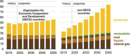
Renewable energy is becoming more important in cities and rural areas due to the high demand for energy in recent decades for residential and commercial purposes, especially in remote areas such as Islands located very far from government power plants (Daryanto 2007). Previous studies showed that 31% of energy is consumed through transportation, while residential and commercial buildings use nearly 40–42% (Cao, Xilei, and Liu 2016) and have the greatest total essential energy consumed in the USA and EU (IEA 2004b). Moreover, the Energy Efficiency Division of the Philippines DOE (2002) showed that 15–20% of the total national energy in the country was consumed by buildings and industries, while a higher percentage of 66% was reported in California, USA (California Energy Commission, 2005). It was also predicted that the energy needed by this sector from different sources in countries that are not members of the Organization for Economic Cooperation and Development Countries (OECD) between 2010 and 2050 is expected to increase from 50 quadrillions BTU to approximately 32–82 quadrillion BTU, while the value required by OECD members is expected to be from 7 quadrillions BTU to approximately 48–55 quadrillion BTU as indicated in Figure 1.

Figure 1. Energy consumption in buildings by many energy resources (2010–2050).

Source: U.S. Energy Information Administration. International Energy Outlook 2019

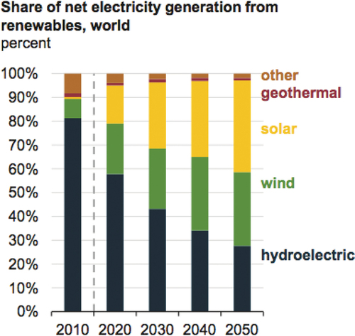
This means more renewable energy is needed to generate and harvest sustainable electricity for residential and commercial or rental office buildings, considering the small quantity it presently contributes when compared to the normal fossil oil as indicated in Figure 1. Countries of the world are observed to be constructing and consuming renewable energy, especially from solar and wind sources, as indicated by the annual average increase of 3.6% from 2018 to 2050 and a gradual decrease in coal-based energy consumption from 35% in 2018 to 22% at the end of 2050. This means coal is the current primary source, while renewable energy is projected to contribute 50% of the total world electricity production in 2050 (International Energy Outlook, 2019). It is also important to note that Building Integrated Photovoltaics System (BIPV) through thousands of solar cells has also been installed across the world from 2013 to 2019 to generate around 5.4 GW and annual growth of 18.7% (Attoye et al., 2018).

The objective of this research was to propose and obtain renewable energy on building facades using honeycomb module wind turbines (Figure 2).

Figure 2. World net electricity production from renewable sources (2010–2050).

Source: U.S. Energy Information Administration. International Energy Outlook 2019

2. Renewable energy

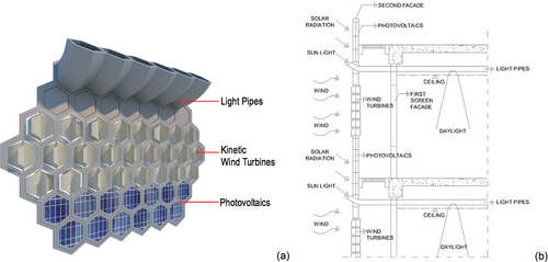
The focus of this research is on renewable energy from solar and wind sources using a smart energy honeycomb façade. This façade depends on a double skin façade which has three parts that include the upper-part hexagonal module in the form of a series of horizontal light pipes built on room ceilings to tap energy from daylight. The middle-part honeycomb module façades consist of thousands of micro-wind turbines to tap energy from kinetic wind sources, while the bottom-part hexagonal modules include thousands of photovoltaic cells used to harness energy from solar radiation as indicated in Figure 3(a and b).

Figure 3. (a) Conceptual double skin smart façade (light-pipes, wind turbines, photovoltaic cells). (b) Schematic building section-drawing showing features of light pipes, wind turbines, and photovoltaics.

2.1. Biomimicry smart façade concept

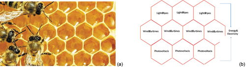
The common double facade building technique applied has been reported to be very effective for energy conservation for a long period (Ahmed et al. 2016). It is also designed to save energy and assist in the process of collecting renewable energies as a contribution to finding solutions to the world energy crisis. Moreover, the idea of using the honeycomb form or bio-mimicry was based on the (1) regular modular to represent the rigidity of the facade structure, and (2) each hexagon module is filled with honey that serves as the source of life for children of bees known as larvae and the queen bees as indicated in Figure 4(a). This design is projected to retrieve renewable electricity using thousands of small windmills placed in one-third of the smart facade as shown in Figure 4(b) while solar cells are on the lower part and the hexagon-shaped reflection pipes are at the top as indicated in Figure 3(a).

Figure 4. (a) Honeycomb, bees, and honey. (b) Honeycomb smart façade module and electricity.

The term BIPV (Building Integrated Photovoltaic) is normally used to define buildings incorporated with PV circuits on the roof or envelope system. IBIPV systems can be used to replace roofing, curtain walls, glazing, or special elements such as eaves or canopies. It is usually applied in the concept of green architecture as an energy-saving strategy through the utilization of solar radiation, which is an environmentally friendly renewable energy source (Howells and Roehrl 2012). Meanwhile, Building Integrated Wind Turbine (BIWT) is a building designed using wind turbines in the facades to produce energy (Arteaga-López, Ángeles-Camacho, and Bañuelos-Ruedas 2019).

2.2. Renewable wind turbines energy systems

An example of renewable energy from wind is the windmill that can be divided into horizontal and vertical types. These two types have the same mechanism and this involves the wind moving the propeller, which later drives the motor to produce electrical energy but the difference is observed from the placement of the quite heavy motor. It is, however, important to note that the vertical type is more advantageous due to its ability to match the weight of gravity that is straight down. Moreover, the movement of the propeller on the wind turbine due to kinetic energy as the wind pushes its surface depends on its horizontal or vertical placement. This classification was also observed in the rotation of the shaft as indicated by the one rotating vertically when the rotor is located in a horizontal position as well as the horizontal rotation when the rotor was placed vertically which has been further developed into Savonius, Darrieus, and H-Rotor as indicated in Figure 5(a).

Figure 5. (a) Horizontal and vertical rotating propeller placement. (b) Principles of wind turbine movement in the Savonius System.

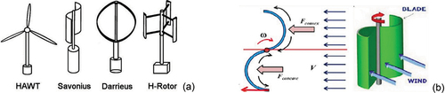
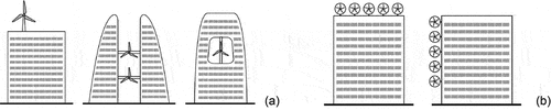
The wind turbine spins due to the difference in pressure on each blade. For example, one of the sunken sides of the Savonius vertical wind turbine captures the wind and spins it, while the other side of the convex receives also wind and causes the turbine to spin as shown in Figure 5(b) (Wenehenubun, Saputra, and Sutanto 2015). It is possible to turn the wind turbines in tall buildings over using two systems. The first involves using several large wind turbines placed on the roof of a building, between two adjacent buildings, or in a hole created inside the building as indicated in Figure 6(a) and this design can be found in the World Trade Center building in Bahrain. The second method uses many small wind turbines installed on buildings as shown in Figure 6(b) and this is considered advantageous due to the fact that the size of the turbines reduces its ability to overload the building structure but requires to be installed in high number to produce the energy needed. An example of these designs can be found in the Miami Coral Tower in Miami (Park et al. 2015). Meanwhile, Savonius VAWT (S-VAWT) is a good candidate due to its high initial torque, low cost, easy installation and repair, and sturdiness (Manwell, McGowan, and Rogers 2010, 1–3).

Figure 6. (a) Three Building Integrated Wind Turbine (BIWT) systems using large wind turbines. (b) Two BIWT systems use small sized wind turbines. (Source: Elger et al., 2015).

3. Methodology overview

The purpose of this research was to obtain the maximal values of electrical power from wind turbines’ hexagonal frame smart façade module. The study is focused on redesigning the wind turbine blades numerically, after which they were simulated using ANSYS Fluent, which is a simulated computational fluid dynamic (CFD) analysis program.

The previous experimental design of the Savonius wind turbine with four blades was used as the basis for the experimental model tested in the wind tunnel at the Mechanical Engineering laboratory and the C_p was found to be only 0.003426. Meanwhile, one module of hexagonal windmill produced 2.30 V, 0.05 A, and 0.1182 W when the wind speed was 4 m/s, while the values were 3.39 V, 0.01 A, and 0.0607 W at 5 m/s (Mintorogo, Elsiana, and Budhiyantho 2019).

3.1. Shape and size of integrated windmills in the building façade

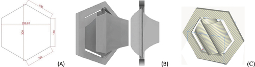
The facade in the building has a small windmill dimension known as a micro-wind turbine, with the longest diameter being 0.30 m while the shortest was 0.25981 m. Moreover, the total area of the hexagons was 0.0585 m² as indicated in Figure 7(a). The “Savonius” Windmill was selected based on the consideration that it is the simplest method and works based on the differences in shear force or differential drag windmill as shown in Figure 7(b and c).

Figure 7. (a) Dimension of honeycomb windmill module. (b) Previous design of savonius wind turbine model. (c) Optimized Savonius wind turbine module with four blades.

3.2. Basic theory for the wind turbine

Turbines are devices used to convert kinetic energy from the wind into motion energy. The amount of energy or turbine power (P) can theoretically be written as follows:

(1) $\mathrm{P}=\mathrm{T}\omega$(1)

Where:

P = Turbine power (W)$\left(watt\right)$.

T = Torque or moment of the turbine (Nm)$\left(Nm\right)$.

ω = Angular velocity of the turbine (rad/s).

The area passed by the air was designed to have the same boundary end to the end and used as a reference value in the ANSYS Fluent 12.0 to determine the moment coefficient. Meanwhile, the dimensionless moment coefficient in line with Rahman et al. (2018, 13) is, therefore, stated as follows:

(2) $C_m=\frac{T}{\frac{1}{4}{V}^2}$(2)

Where:

$C_m$ = Moment coefficient.

$\rho$ = Fluid density (kg/m³).

$A$ = Turbine blade cross-sectional area$\left(m^2\right)$.

D = Diameter of the turbine $\left(m\right)$.

V = Fluid velocity (m/s).

The aerodynamics of turbines also consist of several forces known as dimensionless forces, such as the density and speed of the freestream body. The relationship between these two values is, however, expressed as a dynamic pressure and represented using the following equation.

(3) $q_{\mathrm{\infty }}=\frac{1}{2}{\rho }_{\mathrm{\infty }}{V_{\mathrm{\infty }}}^2$(3)

This means it is possible to define the dimensionless force as follows:

Lift coefficient: $C_L=\frac{L}{q_{\mathrm{\infty }}S}$

Drag coefficient: $C_D=\frac{D}{q_{\mathrm{\infty }}S}$

Normal force coefficient: $C_N=\frac{N}{q_{\mathrm{\infty }}S}$

Axial force coefficient: $C_A=\frac{A}{q_{\mathrm{\infty }}S}$

Where:

L = Lifting force $\left(N\right)$

D = Drag force $\left(N\right)$

N = Normal force $\left(N\right)$

A = Axial force $\left(N\right)$

S = Extensive reference area $\left(m^2\right)$

The S or reference area in the coefficient was selected based on the shape of the body geometry and the values for different shapes are presented in Table 1.

Table 1. C_d values for different body shapes.

Type of Body		Length Ratio	Re	Cp
	Rectangular plate	l/b = 1	>10^4	1.18
		l/b = 5	>10^4	1.20
		l/b = 10	>10^4	1.30
		lb = 20	>10^4	1.50
		l/b = ∞	>10^4	1.98
	Circular Cylinder with ax parallel to flow	l/d = 0 (disk)	>10^4	1.17
		l/d = 0.5	>10^4	1.15
		l/d = 1	>10^4	0.90
		l/d = 2	>10^4	0.85
		l/d = 4	>10^4	0.87
		l/d = 8	>10^4	0.99
	Square rod	∞	>10^4	2.00
	Square rod	∞	>10^4	1.50
	Triangular cylinder	∞	>10^4	1.39
	Semicircular shell	∞	>10^4	1.20
	Semicircular shell	∞	>10^4	2.30
	Hemispherical shell		>10^4	0.39
	Hemispherical shell		>10^4	1.40
	Cube		>10^4	1.10
	Cube		>10^4	0.81
	Cone-60° vertex		>10^4	0.49
	Parachute		≈.3 × 10^7	1.20

Elger et al. (2015, 371–372)

It is possible to capture some of the kinetic energy passing through the turbine cross-section and this is expressed as the power coefficient (C_p) which can be calculated using the following formula:

(4) $C_p=\frac{P}{\frac{1}{2}{V}^3}=\frac{T\omega }{\frac{1}{2}{V}^3}=\lambda C_m$(4)

Where:

$C_p$ = power coefficient

P = power of the turbine (W).

The power coefficient of this turbine, however, depends on the Tip–Speed Ratio (TSR) which is the ratio of blade speed at the tip to the speed of airflow, as indicated in the following relationship:

(5) $\lambda =\frac{\omega R}{V}$(5)

Where:

$\lambda$ = Tip–speed ratio

$R$ = Turbine radius $\left(m\right)$

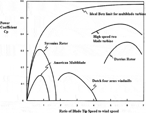
The theoretical power coefficient limit is 0.59 and this is known as the Betz Limit. Meanwhile, Figure 8 shows the maximum value of the power coefficient ($C_p$) against TSR for different types of turbines (Kumar and Saini 2016, 293)

Figure 8. Power coefficient against TSR.

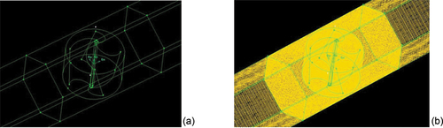
3.3. Simulation validation

The validation process was conducted using a 3D model in accordance with Ferrari et al. and this involved the Savonius turbine model being in line with the Rotor C geometry (Ferrari et al. 2017). Moreover, the Reynolds number used was based on turbine diameter (D_t) and bulk velocity (U_inf), which was 4.32, .105, while the wind tunnel was in line with the method applied by Blackwell et al., and the 1.4% turbulence Intensity used was in accordance with 1% recommended by Suchde et al. (2017, 255). The two simulations conducted with the experimental results of Blackwell, Sheldahl, and Feltz (1977) in the wind tunnel showed that the most optimal Savonius turbine was found at approximately TSR 0.85 with a maximum coefficient of power (C_p) value of 0.25 as indicated in Figure 9. The other TSR variables used based on the angular velocity of the rotor turbine include 0.576, 0.804, and 1.002, while the coefficient of power value was used for comparison. Moreover, the experimental trend of the Savonius turbine performance was presented through the simulation conducted using Ansys Fluent 16.0 with 3D Dimensional, Double Precision, Pressure-Based Solver, Steady-State Condition, and Criteria Convergency 10–5. The Cell Zone conditions were also divided into static and dynamic frames with the dynamic conditions specifically having the frames of motion with rotational velocity.

The simulation results of hexagonal micro-wind turbine were compared with the Ferrari et al. findings, and this study was discovered to have a smaller C_p due to its use of a mathematical model approach that led to some flow phenomena such as the turbulent flow, which was observed to have been developing continually up to the present moment. Sutrisno, Sasongko, and Noor (2015) reported turbulence intensity as an energy reserve being converted gradually to flow and this means the flow with high turbulence tends to have stronger energy. Meanwhile, another flow phenomenon known as the swirl flow was reported by Simanjuntak et al. (2019) to have the capability to be used as a major factor in the coal drying process due to its ability to separate steam vapor in soil coal. The Savonius turbine simulation, however, used very strong turbulence and swirl flow phenomena, thereby, causing high uncertainty.

Figure 9. Comparison between the simulation results of hexagonal micro wind turbine to Ferrari et al. and Blackwell et al.

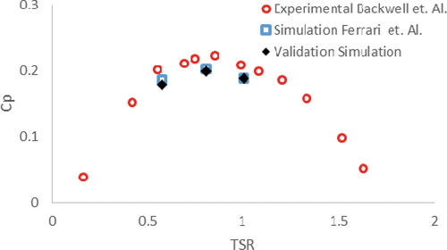
The validation results of hexagonal micro-wind turbine showed large error values of 10.45%, 10.02%, and 9.43% at TSR 0.576, 0.804, 1.002, respectively, as presented in Table 2. This means that the model was unable to produce better predictions than Ferrari et al.’s prediction of the experimental results of Blackwell et al. due to its use of a steady-state condition. It was, therefore, recommended that the unsteady state simulation approach, which requires resource computation with high-performance equipment, should be used in further studies. Meanwhile, some other parameters were selected for the next process, which involved optimizing the hexagonal turbine design. This validation method only compares one parameter due to the focus of this study on the optimization of a new design for the Savonius turbine shape.

Table 2. Comparison of the simulation validation result with the experiment of the Blackwell, Sheldahl, and Feltz (1977).

TSR	Simulation Validation	Error % Cp with Experiment Blackwell et al.
0.576	0.1791	10.45
0.804	0.1994	10.02
1.002	0.1883	9.43

4. Results and discussion

The software used for simulation was ANSYS FLUENT 16.0 using the following parameters:

Viscous model: RNG k-epsilon, Standard Wall Function.

Rotational velocity: varied to obtain a different TSR

Velocity inlet: 4 m/s

Turbulent method: Intensity and length scale

Turbulent length scale: 0.001 m

Turbulent intensity: 5% depend on wind tunnel

3D model and meshing: gambit software (Figure 10).

Figure 10. (a) Savonius 3D facet 3D model. (b) Savonius 3D meshing model.

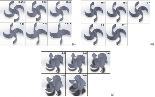
There is a variation in the radius, offset, and twist of the hexagonal or honeycomb wind turbine blades used. The simulation was conducted to obtain the value of the Power Coefficient for the Savonius hexagonal wind turbine using six radii, which include 57.5 mm, 58 mm, 60 mm, 64 mm, 72 mm, and 87.4 mm as shown in Figures 11(a), five offsets including 0 mm, 5 mm, 7 mm, 9 mm, and 11 mm as indicated in Figure 11(b), and the five twist models including 0°, 30°, 45°, 60°, and 90° as presented in Figure 11(c). The design was simulated until the results converge. Moreover, a Y + check was also performed and the value was discovered not to exceed 500 (Tahani et al. 2016, 464), while flux conservation at the inlet and outlet also produced values below 1% and these were considered to be good (Suchde et al. 2017, 255).

Figure 11. (a) Variation in the radius of the turbines. (b) Variation in offset of the turbines. (c) Variations in twist of the turbines.

Table 2 and Figure 12(a and b) show that the optimal value of the turbine blade was found at 58 mm radius with 0.5 TSR, which produced 2.84 W of power and torque of 0.099 Nm as indicated in Table 3, while the power coefficient (C_p) was 0.2786. The model of flow and turbulence kinetic energy produced are presented in Figure 11(a and b).

Figure 12. (a) Vector velocity of wind flow on a 58 mm radius turbine. (b) Turbulent kinetic energy in a 58 mm radius turbine.

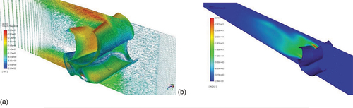
Figure 13. Variants of turbine blade radius.

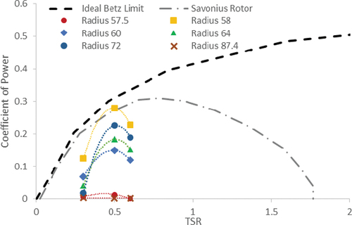
Table 3. Variations in turbine blade radius.

Radius (mm)	TSR	CP	Power (W)	Torque (Nm)	Y Plus
57.5	0.3	0.0063	0.01414182	0.001355268	83.13049
	0.5	0.01362	0.138701848	0.004817709	132.4085
	0.6	0.00102	0.006001218	0.000208448	112.7113
58	0.3	0.12423	0.278864743	0.026724749	85.26819
	0.5	0.2786	2.837076273	0.098543809	132.8681
	0.6	0.22797	1.338171874	0.04648044	112.3835
60	0.3	0.06798	0.152605393	0.014624799	88.38058
	0.5	0.14847	1.511890424	0.052514429	134.181
	0.6	0.11964	0.702281366	0.02439324	113.8718
64	0.3	0.04071	0.091376894	0.008757022	94.81096
	0.5	0.18333	1.866906431	0.064845656	144.2127
	0.6	0.15165	0.890188959	0.030920075	122.4319
72	0.3	0.01791	0.040192929	0.003851853	102.9334
	0.5	0.22628	2.304257532	0.080036733	156.9534
	0.6	0.18799	1.10346569	0.038328089	133.3397
87.4	0.3	0.00319	0.007153723	0.000685571	111.8106
	0.5	0.00312	0.031819299	0.001105221	184.3163
	0.6	0.00266	0.015604645	0.000542016	156.7907

Figure 13 shows that the three models with 58 mm, 64 mm, and 72 mm radius, and the highest C_P values have the same flow velocity patterns. It was also discovered that a smaller drag flow was produced when the radius was fixed and this is less favorable for the performance of the turbine. Moreover, a larger radius produced a larger counter-rotating-vortices flow, which is also less favorable for performance due to its smaller overlap flow. However, the greatest turbulent kinetic energy distribution in the rotor was found in turbines with the smallest diameter, which was 58 mm. This means that a larger diameter of the rotor produced the smaller distribution of turbulent kinetic energy as presented in Figure 12(b).

Table 4 and Figure 14(a and b) show the optimal value of the turbine blade was produced at 11 mm offset with 0.5 TSR as indicated by the production of 3.05 W of power, 0.106 Nm of torque, and 0.29918 power coefficient (C_P). The model of flow and turbulence kinetic energy produced are presented in Figure 13(b).

Figure 14. (a) Vector velocity of wind flow on an 11 mm offset turbine. (b) Turbulent kinetic energy in turbine offset 11 mm.

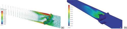
Figure 15. Variants of turbine blade offset (Source: Author).

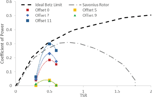
Table 4. Variations in turbine blade offset.

Offset (mm)	TSR	CP	Power (W)	Torque (Nm)	Y Plus
0	0.3	0.04071	0.091377	0.008757	94.81096
	0.5	0.18333	1.866906	0.064846	144.2127
	0.6	0.15165	0.890189	0.03092	122.4319
5	0.3	0.00095	0.002122	0.000203	87.08589
	0.5	0.04072	0.414702	0.014404	132.0764
	0.6	0.00335	0.019688	0.000684	112.0743
7	0.3	0.04683	0.105127	0.010075	84.6218
	0.5	0.22955	2.337588	0.081194	128.1884
	0.6	0.17445	1.023987	0.035567	108.7234
9	0.3	0.01217	0.027321	0.002618	82.36165
	0.5	0.03606	0.367162	0.012753	124.5991
	0.6	0.00611	0.035872	0.001246	105.5825
11	0.3	0.06421	0.144118	0.013811	80.24362
	0.5	0.29918	3.046607	0.105822	121.2431
	0.6	0.250932	1.472946	0.051162	102.7176

Figure 15 shows that the three models with 11, 7, and 0 offsets with the highest C_P values have almost the same flow velocity patterns. A smaller drag flow was produced when the offset was reduced and this is less favorable to the performance of the turbine and the same was also observed for smaller offsets, which caused a greater counter-rotating-vortices flow and smaller overlap flow. Meanwhile, a greater offset of the rotor was observed to cause a smaller distribution of turbulent kinetic energy before it increased again.

Table 4 and Figure 16 show that the optimal value of the turbine blade was at 0-degree twist with 0.5 TSR, which produced 4.75 W of power, 0.165 Nm of torque, and 0.4665 of power coefficient. The model of the flow and turbulence kinetic energy produced is presented in Figure 16(b).

Figure 16. (a) Vector speed of wind flow on turbine twist 0°. (b) Turbulent kinetic energy in turbine twist 0°.

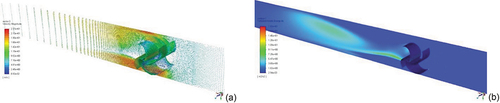
Figure 17. Variants of turbine blade twist.

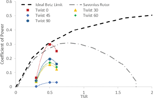
Figure 17 shows the three models 0, 90, and 60 twists with the highest C_P values have almost the same flow velocity patterns. It was discovered that the minimized twist produced a smaller drag flow, and this is less favorable for the performance of the turbine due to its larger counter-rotating-vortices flow. A bigger twist also caused smaller overlap flow, which is also considered less favorable and this means a greater twist of the rotor usually leads to a higher distribution of turbulent kinetic energy before the distribution shrinks again (Table 5).

Table 5. Variations in turbine blade twist.

Twist (degree)	TSR	CP	Power (W)	Torque (Nm)	Y Plus
0	0.3	0.06421	0.144118	0.013811	80.24362
	0.5	0.29918	3.046607	0.105822	121.2431
	0.6	0.250932	1.472946	0.051162	102.7176
30	0.3	0.0367	0.082452702	0.00790178	73.73257
	0.5	0.15497	1.578151371	0.054815956	113.7554
	0.6	0.12406	0.728239091	0.025294862	97.44502
45	0.3	0.00339	0.007624782	0.000730714	74.97164
	0.5	0.03044	0.309972006	0.010766655	113.4298
	0.6	0.03041	0.178473013	0.006199132	96.20094
60	0.3	0.03888	0.087283209	0.008364707	72.77678
	0.5	0.1699	1.730730969	0.060115699	112.8925
	0.6	0.13926	0.817438314	0.028393134	97.33451
90	0.3	0.0441	0.099087932	0.009496002	62.60502
	0.5	0.1949	1.984248782	0.068921458	98.08689
	0.6	0.1599	0.938463598	0.03259686	85.9093

The simulation further combined 58 mm radius, 11 mm offset, and 0° twist and the optimal result was also recorded at TSR 0.5 as indicated by 3.046607 W power, 0.105822 Nm torque, and 0.29918 Power Coefficient (C_P) produced (Table 6 and Figure 18).

Figure 18. Hexagonal turbine optimum model.

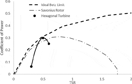
Table 6. Variations in turbine blade TSR.

TSR	CP	Power (W)	Torque (Nm)	Y Plus
0.3	0.06421	0.144118	0.013811	80.24362
0.5	0.29918	3.046607	0.105822	121.2431
0.6	0.25093	1.472946	0.051162	102.7176

5. Conclusions

Numerical and CFD simulations were used to analyze the three parts of designing and optimizing the honeycomb module of Savonius micro-wind turbine with four blades on the second façade building using radius, twist, and offset as the important factors to determine the performance.

The use of 58 mm radius, 11 mm offset, zero-degree twist blade, and 0.5 TSR in the one-piece module design of the micro-hexagonal wind turbine were found to have produced 3.047 W of electricity, which eliminated the piece modules of honeycomb photovoltaics (as explained in the next research), while the optimal Power of Coefficient (C_p) was 0.29918.

The comparison of the Savonius turbine with the Hexagonal Turbine at a TSR of 0.5 showed that the Hexagonal Turbine has a lower TSR leading to a smaller U_inf requirement. This prediction is associated with the four blades used in the design that is more than the Savonius turbine, thereby, causing an increment in the solidity, which is more important for the VAWT than the HAWT. It is also pertinent to note that the high solidity reduces the operating rotation of the wind turbine. Moreover, the C_p value of the Hexagonal Turbine was also found to be higher and closer to the Betz limit, which is the maximum allowed for wind turbines.

The previous design of Hexagonal Savonius with four blades at 90 mm radius, as well as unknown offset and twist, which was tested in wind tunnel, produced only 0.03426 power of coefficient (C_p) and 0.12 W of electricity. This, therefore, means that numerical and CFD simulation was successfully used to determine the optimal blade radius, offset, and twist to produce renewable energy in hexagonal micro-wind turbine architectural building façade.

Disclosure statement

No potential conflict of interest was reported by the author(s).

References

- Ahmed, M. M. A., A. K. A. Rahman, A. H. H. Ali, and M. Suzuki. 2016. “Double Skin Façade: The State of Art on Building Energy Efficiency.” Journal of Clean Energy and Technologies 4 (1): 84–89. doi:10.7763/JOCET.2016.V4.258.
- Arteaga-López, E., C. Ángeles-Camacho, and F. Bañuelos-Ruedas. 2019. “Advanced Methodology for Feasibility Studies on Building-mounted Wind Turbines Installation in Urban Environment: Applying CFD Analysis.” Energy 167: 181–188. doi:10.1016/j.energy.2018.10.191.
- Attoye, D. E., T. O. Adekunle, K. Tabet Aoul, and A. Hassan. 2018. “Building Integrated Photovoltaic (BIPV) Adoption: A Conceptual Communication Model for Research and Market Proposals.” A Conference Proceeding ASEE Connecticut, USA.
- Blackwell, B., R. Sheldahl, and L. Feltz. 1977. “Wind Tunnel Performance Data for Two and Three Bucket Savonius Rotors.” Journal of Energy 2 (3): 160–164.
- California Energy Commission. 2005. “Options for Energy Efficiency in Existing Buildings.”
- Cao, X. D., D. Xilei, and J. Liu. 2016. “Building Energy-Consumption Status Worldwide and the State-of-the-Art Technologies for Zero-Energy Buildings during the past Decade.” Energy and Building 128: 1–58. doi:10.1016/j.enbuild.2016.06.089.
- Coyle, E. D., W. Grimson, B. Basu, and M. Murphy. 2014. “Understading the Global Energy Crisis.” In Book Chapter Part 1: Reflection on Energy, Greenhouses Gases, and Carbonaceous Fuels. Purdue University Press.
- Daryanto, Y. 2007. Kajian Potensi Angin Untuk Pembangkit Listrik Tenaga Bayu. Yogjakarta: BALAI PPTAGG – UPT – LAGG.
- Dudley, N. 2008. “Climate Change and the Energy Crisis. Back to the Energy Crisis – The Need for a Coherent Policy Towards Energy Systems.” Policy Matters 16: 12–68.
- Elger, D. F., B. A. LeBret, C. T. Crowe, and J. A. Robertson. 2015 ed. Barbara, C.W. Engineering Fluid Mechanics. 9th (New York.: John Wiley & Sons)
- Ferrari, G., D. Federici, P. Schito, F. Inzoli, and R. Mereu. 2017. “CFD Study of Savonius Wind Turbine: 3D Model Validation and Parametric Analysis.” Journal of Renewable Energy 105: 722–734. doi:10.1016/j.renene.2016.12.077.
- Howells, M., and R. A. Roehrl. 2012. Perspective on Sustainable Energy for the 21th Century (SD21). New York: United Nations Department of Economic Social Affairs, Division for Sustainable Development.
- IEA. 2004b. Energy Balances for OECD Countries and Energy Balances for Non-OECD Countries, Energy Statistics for OECD Countries and Energy Statistics for Non-OECD Countries. 2004 ed. Paris.
- Kumar, A., and R. P. Saini. 2016. “Performance Parameter of Savonius Type Hydrokinetic Turbine: A Review.” Journal of Renewable and Sustainable Energy Reviews 64: 289–310. doi:10.1016/j.rser.2016.06.005.
- Manienyen, V., M. Thambidurai, and R. Selvakumar. 2009. “Study on Energy Crisis and the Future of Fossil Fuels.” Proceeding of SHEE, Engineering Wing, DDE, Annamalai University, 11–12 December.
- Manwell, J. F., J. G. McGowan, and A. L. Rogers. 2010. Wind Energy Explained: Theory, Design and Application. 2nd ed. Wiley.
- Mintorogo, D. S., F. Elsiana, and A. Budhiyantho. 2019. “Experimental Sustainable Micro Wind Turbines on Second Façade of Buildings.” A Research Report. Center for Research, Petra Christian University.
- Nowak, D. J., E. J. Greenfield, and R. M. Ash. 2019. “Annual Biomass Loss and Potential Value of Urban Tree Waste in the United States.” Urban Forestry & Urban Greening 46: 126469, June 2020. doi:10.1016/j.ufug.2019.126469.
- Park, J., H. J. Jung, S. W. Lee, and J. Park. 2015. “A New Building-Integrated Wind Turbine System Utilizing the Building.” Energies 8 (10): 11846–11870. doi:10.3390/en81011846.
- Rahman, M., T. E. Salyers, A. El-Shahat, M. Ilie, M. Ahmed, and V. Soloiu. 2018. “Numerical and Experimental Investigation of Aerodynamic Performance of Vertical-Axis Wind Turbine Models with Various Blade Designs.” Journal of Power and Energy Engineering 6 (5): 13–14. doi:10.4236/jpee.2018.65003.
- Simanjuntak, M. E., Prabowo, W. A. Widodo, Sutrisno, and M. B. H. Sitorus. 2019. “Experimental and Numerical Study of Coal Swirls Fluidized Bed Drying on 10 ° Angle of Guide Vane.” Journal of Mechanical Science and Technology 33 (11): 5499–5505. doi:10.1007/s12206-019-1042-2.
- Suchde, P., J. Kuhnert, S. Schröder, and A. Klar. 2017. “A Flux Conserving Meshfree Method for Conservation Laws.” International Journal for Numerical Methods in Engineering 112 (3): 238–256. doi:10.1002/nme.5511.
- Sutrisno, M. H., H. Sasongko, and D. Z. Noor. 2015. “Study of the Secondary Flow Structure Caused the Additional Forward-facing Step Turbulence Generator.” Advances and Applications in Fluid Mechanics 18 (1): 129–144. doi:10.17654/AAFMJul2015_129_144.
- Tahani, M., N. Babayan, S. Mehrnia, and M. Shadmehri. 2016. “A Novel Heuristic Method for Optimization of Straight Blade Vertical Wind Turbine.” Energy Conversion and Management 127: 461–476. doi:10.1016/j.enconman.2016.08.094.
- Wenehenubun, F., A. Saputra, and H. Sutanto. 2015. “An Experimental Study on the Performance of Savonius Wind Turbines Related with the Number of Blades.” Energy Procedia 68: 297–304. doi:10.1016/j.egypro.2015.03.259.