Comprehensive system limit state function model and its application for CRTS II track slab

ABSTRACT

Considering safety and serviceability simultaneously, a comprehensive system limit state function (LSF) model and its application for CRTS II track slab is analyzed. First, a comprehensive system LSF model is proposed, and the procedure of comprehensive system reliability analysis is developed from integrating the method of moments with finite element (FE) code. Second, based on the proposed model, comprehensive system LSF of CRTS II track slab is constructed, considering five important safety failure modes and three important serviceability failure modes. Then, comprehensive system reliability of a CRTS II track slab on simply supported viaduct is analyzed using the proposed method, and the result is compared with general system reliabilities considering safety and serviceability separately. It is found that the proposed comprehensive system LSF model has a flexible form and the proposed methodology can be efficiently applied for comprehensive system reliability assessment. It is also found that comprehensive system reliability analysis is more appropriate compared with general system reliability analysis, and thus, comprehensive system reliability results can help to determine an appropriate maintenance strategy and ensure the safety operation for high-speed trains.

KEYWORDS:

• Comprehensive system limit state function
• CRTS II track slab
• system reliability analysis
• ultimate limit state
• serviceable limit state

1. Introduction

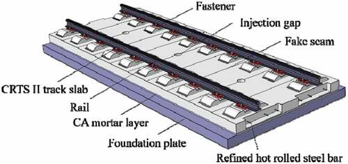
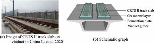
China railway track system II (CRTS II) slab-type ballastless track system has been widely constructed in China’s high-speed railways, which includes the rail, CRTS II track slab, cement asphalt (CA) mortar layer, and foundation plate, as shown in Figure 1. CRTS II track slab, a sensitive element of CRTS II slab-type ballastless track system, plays an important role in carrying and transporting the complicated loads. Under the train load and temperature actions, significant deterioration has occurred in CRTS II track slab (such as crack and fatigue), which may generate into different kinds of failure modes. Based on the corresponding limit state (i.e., ultimate and serviceability limit states), the potential failure modes of CRTS II track slab can be categorized as safety and serviceability kinds. Both the safety and serviceability failure modes will influence the ride comfort or even the safety operation of high-speed trains, and thus, it is crucial to conduct appropriate system reliability analysis for the track slab with a thorough consideration of these two kinds of failure modes.

Figure 1. Schematic graph of CRTS II slab-type ballastless track system.

Most studies evaluate the reliability of CRTS II track slab corresponding to only one individual failure mode (Yu and Mao 2017; Li et al. 2020a). Recently, the system reliability of CRTS II track slab considering five safety failure modes has been conducted (Zhang et al. 2021). However, for a reliable operation of high-speed trains, CRTS II track slab is required to be reliable in both safe and serviceable perspectives, which requires the system reliability of CRTS II track slab be evaluated considering both safety and serviceability failure modes. Furthermore, since some safety and serviceability failure modes of CRTS II track slab are correlated, they need to be considered simultaneously for system reliability analysis. System reliability considering safety and serviceability simultaneously has not been conducted in previous studies and is defined as comprehensive system reliability in this study.

There are generally two approaches to investigate system reliability. One uses the individual limit state functions (LSFs) as objective (Cornell 1976; Melchers 1994; Chun, Song, and Paulino 2015; Gong and Zhou 2017; Song and Kang 2009), which will inevitably encounter the problem of complex correlation among different failure modes (Li, Chen, and Fan 2007). To avoid the difficulties of the first approach, the second approach uses the system LSF as objective and conducts the reliability analysis using method of moments (Zhao and Lu 2021) or probability density evolution method (Li, Chen, and Fan 2007). To make a good balance between accuracy and efficiency, method of moments is applied in this study, which is straightforward and easy to combine with finite element (FE) code. Generally, the system LSF is expressed as an extreme function of individual LSFs (Li, Chen, and Fan 2007; Zhao and Lu 2021), which requires the individual LSFs comparable. This can be easily realized by using the unitless model of individual LSFs (Zhang et al. 2021) for reliability considering only one kind of failure modes, where the expected costs for all the failure modes are the same. However, when considering the safety and serviceability failure modes simultaneously in comprehensive system reliability analysis, the expected costs for different kinds of failure modes are different, and thus, the unitless model of individual LSFs cannot be compared directly. Obviously, the existing system LSF model cannot be applied for comprehensive system reliability analysis, and a comprehensive system LSF model needs to be proposed.

In this study, a comprehensive system LSF model is proposed considering safety and serviceability simultaneously, and its application in comprehensive system reliability analysis of CRTS II track slab is investigated. The rest of this paper is organized as follows: first, the comprehensive system LSF model is proposed, and the procedure of comprehensive system reliability analysis by using method of moments is outlined with necessary expressions provided; then, comprehensive system LSF of CRTS II track slab is constructed, considering important safety and serviceability failure modes; and finally, the comprehensive system reliability of the CRTS II track slab of a high-speed railway in China is investigated as an example by using the proposed method, and the result is compared with general system reliability considering safety and serviceability separately. The research results can help to make risk-informed and cost-effective maintenance scheme for CRTS II track slab and thus ensure the safety operation of high-speed trains.

2. Comprehensive System Reliability Analysis Method

2.1. Construction of comprehensive system limit state function

2.1.1. Definition of comprehensive limit state

To construct the comprehensive system LSF considering safety and serviceability simultaneously, the comprehensive system limit state should be discussed first. When an engineering structure is loaded in some way, its response should satisfy some requirements, which may include the safety of the structure against damage limitations, deflections limitations, or any of a range of other criteria. Each of these requirements may be termed as a limit state (Zhao and Lu 2021). The violation of a limit state can then be defined as the attainment of a fail condition for the structure, which means the limit state is the boundary of a fail zone in a specific dimension. The ultimate and serviceability limit states are the boundaries of fail zones for safety and serviceability dimensions. As the comprehensive limit state considers safety and serviceability simultaneously, it is constructed by the union of modified ultimate and serviceability limit states and is corresponding to a newly defined comprehensive dimension. To define a limit state, the target reliability level (represented by the target reliability index) and expected cost for breaking the limit state should be determined, which are generally directly proportional with each other. As the comprehensive limit state should reflect the reliability level for both the safety and serviceability dimension, its target reliability index β_comp should within the range of [β_service,β_safe], where β_service and β_safe are the target reliability indices when considering serviceability and safety, respectively. Correspondingly, the expected cost for breaking the comprehensive limit state C_comp should be within the range of [C_service,C_safe], where C_service and C_safe are the expected costs for breaking serviceability and ultimate limit states, respectively. With different C_comp and β_comp defined, there are many possible comprehensive limit states. For convenience, C_comp is advised to be defined as that of the dominant limit state. Based on C_comp, the ultimate and serviceability limit states can be modified and equivalently transformed into the comprehensive dimension to construct the comprehensive limit state. The modification of a limit state is mathematically reflected by the modification of individual LSFs for corresponding individual failure modes, which will be discussed in the following section.

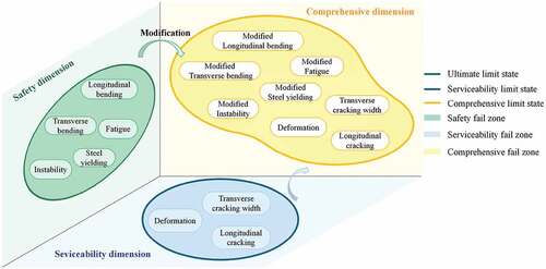
To illustrate the relationship among the ultimate, serviceability and comprehensive limit states, a schematic graph of such relationship for CRTS II track slab is depicted in Figure 2 as an example. The serviceability limit state is dominant in Figure 2, while the individual failure modes corresponding to different limit states will be discussed in section 3. It can be found from Figure 2 that, the comprehensive limit state is different from the ultimate and serviceability limit states. As the serviceability limit state is dominant, the serviceability limit state in the comprehensive fail zone is the same as the original ones, while the ultimate limit state in the comprehensive fail zone are modified from the original ones.

Figure 2. Schematic graph of ultimate, serviceability, and serviceability-dominant comprehensive limit states for CRTS II track slab.

2.1.2. Modified individual limit state function

Since the limit states are modified for comprehensive system reliability analysis, the individual LSFs should be modified from the general ones accordingly. The general form of an individual LSF G(X) is formulated as:

(1) $G(\mathbf{X})=R-S$(1)

where R and S are, respectively, the general resistance and load of G(X). The modification of individual LSF corresponding to the comprehensive limit state is realized by multiplying a modified coefficient α to the general resistance. And then, the modified individual LSF G_M(X) is expressed as

(2) $G_M(\mathbf{X})=\alpha R-S$(2)

As the sign of G_M(X) rather than its absolute value is important in reliability analysis, G_M(X) is equivalently formulated in the unitless form, i.e., G_M(X)/R, for system reliability analysis with multiple units considered (Zhang et al. 2021). Accordingly, the ith modified safety and serviceability individual LSFs, G_MUi(X) and G_MSi(X) are formulated as

(3) $G_{MUi}(\mathbf{X})={\alpha }_{safe}-S_{Ui}/R_{Ui}$(3)

(4) $G_{MSi}(\mathbf{X})={\alpha }_{service}-S_{Si}/R_{Si}$(4)

where α_safe and α_service are the modified coefficients for the safety and serviceability failure modes, respectively; S_Ui and S_Si are the general loads of the ith safety and serviceability failure modes; and R_Ui and R_Si are the general resistance of the ith safety and serviceability failure modes. As the modification of limit states aims to reflect the changing of expected costs, the values of α_safe and α_service are determined as C_comp/C_safe and C_comp/C_service, respectively. As C_comp is advised to be set as the expected cost of dominant limit state, the modified coefficient for the dominant limit state becomes 1, and the other one is determined as its expected cost dividing that of the dominant expected cost. For example, when serviceability is dominant, α_service =1 and α_safe =C_service/C_safe.

Comparing with the general individual LSF as given in Eq. (1(1) $G(\mathbf{X})=R-S$(1) ), the modified individual LSF given in Eq. (3)(3) $G_{MUi}(\mathbf{X})={\alpha }_{safe}-S_{Ui}/R_{Ui}$(3) and (4(4) $G_{MSi}(\mathbf{X})={\alpha }_{service}-S_{Si}/R_{Si}$(4) ) has no change in the general load and resistance, which makes the proposed comprehensive system LSF easily constructed with no limitations.

2.1.3. Comprehensive system limit state function model

As neither the modified ultimate nor the modified serviceability limit state is allowed to be broken, the comprehensive system LSF can be defined based on series system theory (Zhao and Lu 2021) and formulated as

(5) $G_{sys}(\mathbf{X})=min[G_{MU\mathrm{\_}sys}(\mathbf{X}),G_{MS\mathrm{\_}sys}(\mathbf{X})]$(5)

where G_{MU_sys}(X) and G_{MS_sys}(X) are the system LSFs corresponding to the modified ultimate and modified serviceability limit states. With different logical relationships among individual failure modes, a system can be defined as series, parallel or series-parallel. Based on the types of system considering modified individual failure modes, the expressions of G_{MU_sys}(X) and G_{MS_sys}(X) can be determined as follows (Zhao and Lu 2021).

1. Series system

In reliability theory, a series system means the occurrence of one failure mode will constitute the system failure. The system LSF of a series system is expressed as the minimum of all individual LSFs (Zhao and Lu 2021). Thus, when the modified individual failure modes are serially connected, G_{MU_sys}(X) and G_{MS_sys}(X) are formulated as

(6a) $G_{MU\mathrm{\_}sys}(\mathbf{X})=min[G_{M{U}_1}(\mathbf{X}),\dots ,G_{M{U}_i}(\mathbf{X}),\dots ,G_{M{U}_n}(\mathbf{X})]$(6a)

(6b) $G_{MS\mathrm{\_}sys}(\mathbf{X})=min[G_{M{S}_1}(\mathbf{X}),\dots ,G_{M{S}_i}(\mathbf{X}),\dots ,G_{M{S}_n}(\mathbf{X})]$(6b)

• (2) Parallel system

A parallel system will fail only when all the individual failure modes have occurred, the system LSF is expressed as the maximum of all individual LSFs. In this case, G_{MU_sys}(X) and G_{MS_sys}(X) are formulated as

(7a) $G_{MU\mathrm{\_}sys}(\mathbf{X})=max[G_{M{U}_1}(\mathbf{X}),\dots ,G_{M{U}_i}(\mathbf{X}),\dots ,G_{M{U}_n}(\mathbf{X})]$(7a)

(7b) $G_{MS\mathrm{\_}sys}(\mathbf{X})=max[G_{M{S}_1}(\mathbf{X}),\dots ,G_{M{S}_i}(\mathbf{X}),\dots ,G_{M{S}_n}(\mathbf{X})]$(7b)

• (3) Series-parallel system

For reliability analysis, a system is defined as a series-parallel system when it contains a mixture of series- and parallel-connected individual failure modes. The system LSF is formulated based on the specific logical relationship.

2.2. Procedure of comprehensive reliability analysis

Since the comprehensive system LSF is generally constructed with the combination of a FE model in practice, method of moments is applied for comprehensive system reliability analysis. The reliability analysis using this method is conducted by directly constructing the probability distribution of the LSF with its statistical moments as constraints. As the LSF is only calculated several times in evaluating its statistical moments and no derivative calculation is required, method of moments can be efficiently applied for comprehensive reliability analysis including FE code.

The procedure of comprehensive system reliability analysis by using method of moments is summarized in Figure 3, which generally includes four steps. The first step is to construct the individual LSF corresponding to the identified safety and serviceability failure modes, which is similar as other reliability analysis method. Then the comprehensive system LSF G_sys(X) is constructed based on the logical relationship among individual failure modes, where the proposed comprehensive system LSF model (as given in Eq. (3)–(3) $G_{MUi}(\mathbf{X})={\alpha }_{safe}-S_{Ui}/R_{Ui}$(3) (5(5) $G_{sys}(\mathbf{X})=min[G_{MU\mathrm{\_}sys}(\mathbf{X}),G_{MS\mathrm{\_}sys}(\mathbf{X})]$(5) )) is applied instead of the general model. The third and fourth steps are the calculation of statistical moments of G_sys(X) and comprehensive system reliability evaluation, and the details of these two steps are summarized in the following.

1. Third step: Calculation of the statistical moments of G_sys(X)

Figure 3. Procedure of comprehensive reliability analysis using method of moments.

Based on theoretical definition of statistical moments, the mean, standard deviation, skewness and kurtosis of G_sys(X) (i.e., α_G, σ_G, α_3G and α_4G) are expressed as (Xu and Rahman 2004)

(8a) ${\mu }_G=E_{1G}$(8a)

(8b) ${\sigma }_G=\sqrt{E_{2G}-E_{1G}^2}$(8b)

(8c) ${\alpha }_{3G}=\frac{1}{{\sigma }_G^3}(E_{3G}-3E_{2G}{E}_{1G}+2E_{1G}^3)$(8c)

(8d) ${\alpha }_{4G}=\frac{1}{{\sigma }_G^4}(E_{4G}-4E_{3G}{E}_{1G}+6E_{2G}{E}_{1G}^2-3E_{1G}^4)$(8d)

where E_kG (k = 1, …,4) is the kth original moments of G_sys(X). Since G_sys(X) is combined with FE model, direct calculation of E_kG is difficult, and the point estimate method is applied combining with the bivariate dimension-reduction method (BDRM) (Zhao and Lu 2021; Xu and Rahman 2004). Then, E_kG is approximately expressed as

(9a) $E_{kG}\cong \sum _{i=1}^{n-1}\sum _{j>i}^n{E}_{ij}^k-(n-2)\sum _{i=1}^n{E}_i^k+\frac{(n-1)(n-2)}{2}[G_{sys}(\mu ){]}^k$(9a)

(9b) $E_i^k=\underset{r=1}{\overset{m}{\mathrm{\Sigma }}}{P}_r\{G_{sys}[{\mu }_1,\dots ,T(u_r),\dots ,{\mu }_n]{\}}^k$(9b)

(9c) $E_{ij}^k=\sum _{r_i=1}^m\sum _{r_j=1}^m{P}_{r_i}{P}_{r_j}{G}_{sys}{[{\mu }_1,\dots ,T(u_{r_i}),\dots ,T(u_{r_j}),\dots ,{\mu }_n]}^k$(9c)

where n is the number of random variables is the vector of the mean values; m is the number of estimate points; u_r,u_ri,u_rj and P_r,P_ri,P_rj are respectively the abscissa in Gaussian space and corresponding weights; and T(·) is the inverse normal transformation function. Generally, the accuracy of point estimate method can be guaranteed with 5 or 7 estimate points (Zhao and Lu 2021), and u_r and P_r for m = 5 and 7 are listed in Table 1. For random variables with known distributions, T(·) can be defined by the Rosenblatt transformation (Hohenbichler and Rackwitz 1981). For random variables with unknown distributions, Rosenblatt transformation is inapplicable, and the third-order polynomial normal transformation based on the first four moments can be applied alternatively (Fleishman 1978; Ding and Chen 2016).

1. Fourth step: Comprehensive system reliability evaluation

Table 1. Abscissa u_r in Gaussian space and corresponding weight p_r for m = 5 and 7.

Number of estimate points m	Abscissa ur	Weight pr
5	0	0.5333
	±1.3556	0.2208
	±2.8570	0.01126
7	0	0.4574
	±1.1544	0.2401
	±2.3668	0.0308
	±3.7504	0.0005

With the statistical moments of G_sys(X) obtained, the reliability index β can be readily obtained by the fourth moment normal transformation (FMNT) as (Zhao and Lu 2021)

(10a) $\beta =\frac{\sqrt[3]{2}p}{\sqrt[3]{\mathrm{\Delta }-q}}-\frac{\sqrt[3]{\mathrm{\Delta }-q}}{\sqrt[3]{2}}+\frac{a_3}{3a_4}$(10a)

(10b) $\mathrm{\Delta }=\sqrt{q^2+4p^3},p=\frac{3a_2{a}_4-a_3^2}{9a_4^2}$(10b)

$a_2=1-3a_4,$

$a_3=\frac{5+(35-{\alpha }_{3G}^2)a_4^2}{9a_0+30-0.8{\alpha }_{3G}^2}{\alpha }_{3G},$

(10c) $a_4=\frac{2a_0}{2a_0+46(1-1/{\alpha }_{4G}^2)-{\alpha }_{3G}^2}$(10c)

$k=\frac{1}{\sqrt{1+2a_3^2+6a_4^2}},$

(10d) $a_0=\frac{\sqrt{3{\alpha }_{4G}-4{\alpha }_{3G}^2-5}-2}{1-(3{\alpha }_{3G}^2+1)/{\alpha }_{4G}^2}$(10d)

where β_2M is the second-order reliability index. When α_3G and α_4G fall outside the range of Eq. (10a), a complete fourth-moment reliability index (Zhao, Zhang, and Lu 2018) can be applied. It should be noted that the proposed comprehensive system LSF and the comprehensive system reliability analysis method has no limitation for the type of structures. In the following, the application of the proposed model and method in CRTS II track slab will be investigated as an example.

3. Comprehensive system limit state function of CRTS II track slab

3.1. Review of individual limit state functions for important safety failure modes

The important safety failure modes for CRTS II track slab have been investigated (Zhang et al. 2021), including the longitudinal bending, transverse bending, steel yielding, vertical instability, and fatigue. The safety LSFs corresponding to these safety failure modes have been proposed by Zhang (Zhang et al. 2021), which are summarized in the following

Longitudinal bending:

(11) $G_{U1}(\mathbf{X})=1-(M_{fl}+M_{tl}+M_{nq})/M_{ul}$(11)

Transverse bending:

(12) $G_{U2}(\mathbf{X})=1-(M_{fh}+M_{th}+M_L)/M_{uh}$(12)

Steel yielding:

(13) $G_{U3}(\mathbf{X})=1-{\delta }_{sl}/f_{yk}$(13)

Vertical instability:

(14) $G_{U4}(\mathbf{X})=1-{\lambda }_{cr}{F}_{tkc}/{\lambda }_{CA}{P}_{cr}$(14)

Fatigue:

(15) $G_{U5}(\mathbf{X})=1-{\lambda }_D{n}_z/N_z$(15)

where M_fl is the longitudinal bending moment caused by vertical train load, which is determined using FE analysis (details can be found in Appendix A); M_tl and M_nq are the longitudinal moments caused by the temperature gradient T_g and bridge deformation, respectively; M_ul and M_uh are the longitudinal and transverse ultimate bending moments of the track slab; F_tkc is the tensile stress of the concrete caused by axial temperature ΔT; P_cr is the critical unstable pressure; λ_D is the correction factor considering the sensor measurement error and model uncertainty; n_z is the number of cycles of the loads; and N_z = 2.0 × 10⁶ is the maximum cycle of the loads before the track slab fails. The expressions of M_tl,M_nq,M_l,M_ul,M_uh,F_tkc, and P_cr are given as follows:

(16) $M_{tl}=\frac{a_t{a}_h{E}_c{T}_g{h}^4}{12(1-v)},M_{nq}=\frac{E_{c}I\phi \pi }{L_b},M_L=0.3Q{h}_a$(16)

(17) $M_{ul}=f_{sl}{A}_{sl0}(h_a-a_{sl})+f_{sr}{A}_{sr}(h_{ar}-a_{sl}),M_{uh}=f_{sh}{A}_{sh}(h_a-a_{sh})$(17)

(18) $F_{tkc}={\lambda }_c{E}_c{a}_c\mathrm{\Delta }T{A}_g,P_{cr}=\frac{4{\pi }^2{E}_{c}I}{L_l^2}$(18)

where I = bh³/12 is the inertia moment of the track slab, φ is the angle at the beam end; L_b = 20 m is the length of the bridge span; f_sl = f_sr = 435MPa are the tensile strengths of longitudinal steel bars and refined hot rolled steel bars; A_sl0 = 201 mm² and A_sr = 1185 mm² represent the sectional areas of the longitudinal steel bars in tensile zone and the refined hot rolled bars, respectively; h_a = 150 mm and h_ar = 135 mm are the effective height and distance from the bottom to the surface of refined hot bar; a_sl =70 mm is the distance from the longitudinal bars in compressive zone to the edge of the compressive zone; f_sh = 435MPa is the tensile strength of the transverse steel bars; A_sh = 2211.68 mm² represents the cross sectional areas of the transverse steel bars; a_sh = 60 mm is the distance from the compressive steel bars to the top surface of the track slab; λ_cr is the reduction factor reflecting adverse conditions such as initial eccentricity; λ_CA is the increase factor reflecting the influence of CA mortar layer adhesion; L_l represents the effective length of the simulated compressive lever, which is considered as 3l, and l = 6.45 m is the track slab length.

3.2. Individual limit state functions for important serviceability failure modes

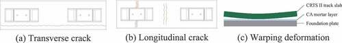
When considering the serviceable limit state of CRTS II track slab, crack and deformation are the objectives to be investigated. There may be transverse, longitudinal and diagonal cracks in the track slab. The mechanism of transverse and longitudinal cracks has been investigated (Tong et al. 2020), while that of the diagonal crack is unclear in this stage. As investigating the mechanism of diagonal crack is not the focus of this study, only the transverse and longitudinal cracks are considered in constructing the comprehensive LSF. The serviceability failure modes of the track slab are then sorted into three kinds, which are the transverse crack width, longitudinal crack, and the warping deformation. These considered serviceability failure modes are schematically shown in Figure 4 (a) -(c), while the general form of the corresponding individual LSFs are discussed in the following.

Figure 4. Schematic graph of serviceability failure modes of CRTS II track slab.

3.2.1. Transverse crack width

Longitudinally, CRTS II track slabs are connected with each other by 6 refined hot rolled steel bar with diameter of 20 mm, and the track slab can be seen as longitudinally continues. As a longitudinal continues structure, the transverse crack is allowed for CRTS II track slab. To guide the transverse crack, V-shape “fake seams” are placed between the bearing platforms, as shown in Figure 1. In practice, under the influence of uncertainties in material and loads, the transverse crack may happen apart from the “fake seams”. The positions of the transverse cracks show significant randomness, which may be the edge of bearing platforms, the edge of injection gaps, overpassing the fastener, etc. The width of the transverse cracks is designed to be within an allowable range, and thus the transverse crack width failure mode refers to the situation when the max width of the transverse crack w_max exceeds the allowable range [w_max]. The corresponding LSF G_S1(X) is constructed as follows

(19) $G_{S1}(\mathbf{X})=1-w_{max}/[w_{max}]$(19)

where [w_max] = 0.4 mm is the allowable width of CRTS II track slab’s transverse crack (Tong et al. 2020); w_max is expressed as (NSPRC 2018)

(20) $w_{max}={\alpha }_{cr}\psi \frac{{\sigma }_{sl}}{E_s}(1.9c_s+0.08\frac{d_{eq}}{{\rho }_{te}})$(20)

where α_cr = 2.4 is the factor reflecting the load character; ψ = 1.0 is the coefficient reflecting the unevenness of the tensile pressure of the steels; d_eq is the equivalent diameter of the longitudinal steel; ρ_te = A_sl/A_g is the longitudinal tension steel ratio; A_g = b·h is the sectional area of the track slab, b =2.55 m and h = 0.2 m are the width and thickness of the track slab, respectively; and c_s = 0.05 m is the thickness of concrete cover in the bottom of the track slab. There are 16 steel rebars set in the transverse direction of CRTS II track slab with a diameter of 8 mm, and thus d_eq is 8 mm and A_sl = 804 mm². σ_sl is the longitudinal tensile stress of the steel bars, which is expressed as

(21) ${\delta }_{sl}={\delta }_{tk}+{\delta }_{ttk}+{\delta }_{ck}+\frac{F_b}{A_{sl}}$(21)

where δ_tk,δ_ttk, and δ_ck are the tensile stresses of the steel bars caused by axial temperature ΔT, temperature gradient T_g, and shrinkage and creep of the concreteΔT_ck, respectively; F_b is the tension of steel caused by the longitudinal train load. The expressions of δ_tk,δ_ttk,δ_ck and F_b are given as

(22) ${\delta }_{tk}={\lambda }_s{E}_s{a}_{ts}\mathrm{\Delta }T$(22)

(23) ${\delta }_{ttk}={\lambda }_s{E}_s{a}_{ts}{T}_{g}h/2$(23)

(24) ${\delta }_{ck}={\lambda }_s{E}_s{a}_{ts}\mathrm{\Delta }{T}_{ck}$(24)

(25) $F_b=n_{cj}{F}_{cj}\frac{A_g{f{ }^{\mathrm{\prime }}}_c}{A_g{f{ }^{\mathrm{\prime }}}_c+A_d{f{ }^{\mathrm{\prime }}}_d}$(25)

where E_s = 200GPa is the elastic modulus of the steel; λ_s = 1/2 is the reduction factor of E_s; a_ts = 1.2 × 10^‒5/°C is the coefficient of linear thermal expansion of the steel; n_cj is the number of fasteners per unit in one rail; F_cj is the resistance of the fasteners; =1.96MPa and =1.43 MPa are, respectively, the tension strengths of track slab and foundation plate; and A_d = 0.59 m² is the sectional area of foundation plate.

3.2.2. Longitudinal crack

Different from the transverse requirement, longitudinal crack is not allowed for CRTS II track slab. The longitudinal crack will occur when the practical transverse moment exceeds the ultimate crack moment M_cr. Therefore, the corresponding LSF G_S2(X) is defined as the relationship between M_cr and the transverse bending moment. As the train load will cause large transverse stress in the track slab (Ou 2016), which may result in the transverse crack, the effects of train load are considered in G_S2(X). Under the temperature gradient T_g, the track slab may have warping deformation, which will also cause longitudinal cracks. And thus the effect of T_g is also considered in G_S2(X). Then, G_S2(X) is formulated as:

(26) $G_{S2}(\mathbf{X})=1-(M_{fh}+M_{th}+M_L)/M_{cr}$(26)

where M_fh is the transverse bending moment caused by the vertical train load, which is determined using FE analysis (details can be found in Appendix A); and M_th and M_L are the transverse moments caused by temperature gradient T_g and transverse train load, respectively. The expressions of M_th and M_L are given as (Zhang et al. 2021)

(27) $M_{th}=\frac{a_t{a}_h{E}_c{T}_g{h}^4}{12(1-v)}$(27)

(28) $M_L=0.3Q{h}_a$(28)

where a_t = 10^‒5/°C is the coefficient of linear thermal expansion; a_h =1.0 is the correction factor of thickness; E_c = 35.5GPa is the elastic modulus of concrete of the track slab; v = 0.2 is the Poisson’s ratio of the track slab; Q = 0.8P_j is the transverse train load, and P_j is the static wheel load. As the value of M_cr is difficult to determine analytically, it is evaluated based on experiments (Zhang 2014).

3.2.3. Warping deformation

Subjected to the temperature gradient, CRTS II track slab may have warping deformation. When the deformation is controlled, there will be temperature stress in the track slab. When the warping deformation is too large, the warping stress σ_q may exceed the ultimate warping stress σ_uq of CA mortar layer and the reliability cannot be guaranteed. The corresponding LSF is expressed as the relationship between σ_uq and σ_q as follows:

(29a) $G_{S3}(\mathbf{X})=1-{\sigma }_q/{\sigma }_{uq}$(29a)

(29b) ${\sigma }_q=\frac{E_c{a}_t{T}_{g}h}{2(1-\nu )}$(29b)

As the warping deformation occurs resulting from the interfacial debonding between the track slab and CA mortar layer, σ_uq is set to be the maximum value of the normal cohesive strength between these two layers, which is approximately 1.792MPa (Liu et al. 2017).

3.3. Construction of comprehensive system limit state function

Combining the proposed modified individual LSF model (Eq. (3)(3) $G_{MUi}(\mathbf{X})={\alpha }_{safe}-S_{Ui}/R_{Ui}$(3) and (4(4) $G_{MSi}(\mathbf{X})={\alpha }_{service}-S_{Si}/R_{Si}$(4) )) with the general individual LSFs given in Eqs. (11)-(29b(29b) ${\sigma }_q=\frac{E_c{a}_t{T}_{g}h}{2(1-\nu )}$(29b) ), the modified safety individual LSF G_{i_U}(X) (i = 1, …,5) and modified serviceability LSF G_{j_S}(X) (j = 1, …,3) are formulated as

(30a) $G_{M{U}_1}(\mathbf{X})={\alpha }_{safe}-(M_{fl}+M_{tl}+M_{nq})/M_{ul}$(30a)

(30b) $G_{M{U}_2}(\mathbf{X})={\alpha }_{safe}-(M_{fh}+M_{th}+M_L)/M_{uh}$(30b)

(30c) $G_{M{U}_3}(\mathbf{X})={\alpha }_{safe}-{\delta }_{sl}/f_{yk}$(30c)

(30d) $G_{M{U}_4}(\mathbf{X})={\alpha }_{safe}-{\lambda }_{cr}{F}_{tkc}/{\lambda }_{CA}{P}_{cr}$(30d)

(30e) $G_{M{U}_5}(\mathbf{X})={\alpha }_{safe}-{\lambda }_D{n}_z/N_z{D}_e$(30e)

(30f) $G_{M{S}_1}(\mathbf{X})={\alpha }_{service}-w_{max}/[w_{max}]$(30f)

(30g) $G_{M{S}_2}(\mathbf{X})={\alpha }_{service}-(M_{fh}+M_{th}+M_L)/M_{cr}$(30g)

(30h) $G_{M{S}_3}(\mathbf{X})={\alpha }_{service}-{\sigma }_q/{\sigma }_{uq}$(30h)

As the occurrence of each modified safety (or serviceability) failure mode implies the failure of CRTS II track slab from the safe (or serviceable) perspective, the track slab is a series system when considering modified ultimate and serviceability limit states separately. Based on Eq. (6a)(6a) $G_{MU\mathrm{\_}sys}(\mathbf{X})=min[G_{M{U}_1}(\mathbf{X}),\dots ,G_{M{U}_i}(\mathbf{X}),\dots ,G_{M{U}_n}(\mathbf{X})]$(6a) and (6b(6b) $G_{MS\mathrm{\_}sys}(\mathbf{X})=min[G_{M{S}_1}(\mathbf{X}),\dots ,G_{M{S}_i}(\mathbf{X}),\dots ,G_{M{S}_n}(\mathbf{X})]$(6b) ), G_{MU_sys}(X) and G_{MS_sys}(X) are constructed as

(31) $G_{MU\mathrm{\_}sys}(\mathbf{X})=min[G_{M{U}_1}(\mathbf{X}),G_{M{U}_2}(\mathbf{X}),G_{M{U}_3}(\mathbf{X}),G_{M{U}_4}(\mathbf{X}),G_{M{U}_5}(\mathbf{X})]$(31)

(32) $G_{MS\mathrm{\_}sys}(\mathbf{X})=min[G_{M{S}_1}(\mathbf{X}),G_{M{S}_2}(\mathbf{X}),G_{M{S}_3}(\mathbf{X})]$(32)

Substituting Eq. (31)(31) $G_{MU\mathrm{\_}sys}(\mathbf{X})=min[G_{M{U}_1}(\mathbf{X}),G_{M{U}_2}(\mathbf{X}),G_{M{U}_3}(\mathbf{X}),G_{M{U}_4}(\mathbf{X}),G_{M{U}_5}(\mathbf{X})]$(31) and (32(32) $G_{MS\mathrm{\_}sys}(\mathbf{X})=min[G_{M{S}_1}(\mathbf{X}),G_{M{S}_2}(\mathbf{X}),G_{M{S}_3}(\mathbf{X})]$(32) ) into Eq. (5(5) $G_{sys}(\mathbf{X})=min[G_{MU\mathrm{\_}sys}(\mathbf{X}),G_{MS\mathrm{\_}sys}(\mathbf{X})]$(5) ), the comprehensive system LSF G_sys(X) for CRTS II track slab can be expressed as

(33) $G_{sys}(\mathbf{X})=min[G_{M{U}_1}(\mathbf{X}),G_{M{U}_2}(\mathbf{X}),G_{M{U}_3}(\mathbf{X}),G_{M{U}_4}(\mathbf{X}),G_{M{U}_5}(\mathbf{X}),G_{M{S}_1}(\mathbf{X}),G_{M{S}_2}(\mathbf{X}),G_{M{S}_3}(\mathbf{X})]$(33)

4. Comprehensive system reliability analysis of CRTS II track slab

To demonstrate the applicability of the proposed comprehensive system LSF model and the comprehensive reliability method, the CRTS II track slab laid on a simply-supported viaduct is taken as an example, as shown in Figure 5. There are multiple units of CRTS II track slab laid on the viaduct, while the track slab in mid-span is the objective of this example.

Figure 5. CRTS II track slab on simply supported viaduct.

With eight failure modes considered, there are plenty parameters in G_sys(X). Based on the randomness of different parameters, 12 parameters are considered as random variables when considering the safety failure modes, which are the P_j, F_cj, T_g, Δ, ΔT, φ, n_z, λ_CA, λ_cr, and λ_D (Zhang et al. 2021). In the comprehensive system reliability analysis, the above mentioned parameters are still considered as random variables. Since M_cr is determined from experiments, it has relatively large randomness and thus is considered as random variable in this study. The distributions and statistical moments of these random variables are listed in Table 2. In practice, the axial temperature ΔT and temperature gradient T_g may be positive or negative, and thus their mean value and standard deviation have two cases, as shown in Table 2.

Table 2. Statistical information of random variables of CRTS II track slab.

Random variables	Distribution	μx	σx	α3x	α4x	Reference
Pj (kN)	Normal	119	26.18	0	3	(MRPRC 2016)
Fcj (kN/m)	Lognormal	12	3.600	0.927	4.566	(MRPRC 2016)
Tg (^oC/m)	Weibull	‒45/90	15.75/31.50	‒0.352	3.004	(MRPRC 2016b)
ΔT (^oC)	Lognormal	±22.5	5.625	0.608	3.664	(MRPRC 2016b)
ΔTck (^oC)	Lognormal	10	1.000	0.301	3.162	(MRPRC 2016b)
φ (rad)	Lognormal	0.001	0.0002	0.608	3.664	(MRPRC 2016b)
nz	Normal	10^6	1.5 × 10^6	0	3	Assumed based on local reports
λCA	Normal	1	0.150	0	3	Assumed based on local reports
λcr	Lognormal	1.25	0.188	0.453	3.368	Assumed based on local reports
λD	Normal	1.2	0.120	0	3	Assumed based on local reports
Mcr (kN.m)	Unknown	52.942	7.094	0.989	3.637	Calculated from experiments (Xu and Rahman 2004)

4.1. Comprehensive system reliability

With the comprehensive system LSF G_sys(X) constructed and the statistical information of random variables determined, the comprehensive system reliability can be evaluated according to Figure 4. Since the mean values of ΔT and T_g, i.e., μ_ΔT and μ_Tg, may be positive or negative, four cases are considered in system reliability analysis:

Case 1: μ_ΔT and μ_Tg are both positive;

Case 2: μ_T is positive while μ_Tg is negative;

Case 3: μ_ΔT is negative while μ_Tg is positive;

Case 4: μ_ΔT and μ_Tg are both negative.

Furthermore, in this section, three different comprehensive limit states are defined to show the influence of dominant limit state, which are serviceability-dominant, safety-dominant, and serviceability-safety dominant (safety and serviceability are equivalent). As the expected costs of serviceable and safe failure modes, i.e., C_service and C_safe, are unknown in this stage, C_service/C_safe is assumed to be 0.95. Accordingly, α_service and α_safe for different comprehensive limit states can be directly determined as: {α_service,α_safe} = {1.0, 0.95} for serviceability dominant; {α_service, α_safe} = {1.05, 1.0} for safety dominant; {α_service, α_safe} = {1.0, 1.0} for serviceability-safety dominant.

The first four moments of G_sys(X), i.e.,μ_G,σ_G, α_3G and α_4G can be directly calculated by using point estimate method combined with BDRM as given in Eq. (8a)(8a) ${\mu }_G=E_{1G}$(8a) -(9c(9c) $E_{ij}^k=\sum _{r_i=1}^m\sum _{r_j=1}^m{P}_{r_i}{P}_{r_j}{G}_{sys}{[{\mu }_1,\dots ,T(u_{r_i}),\dots ,T(u_{r_j}),\dots ,{\mu }_n]}^k$(9c) ). Seven-point estimate method is applied (i.e., m = 7), and the values of μ_G, σ_G, α_3G and α_4G are listed in Table 3. Then, the comprehensive system reliability index β is determined by using Eq. (10a)-(10d), which are also listed in Table 3. For comparison, MCS method (10⁷ samples) is also conducted as a benchmark for the accuracy, with the obtained β also listed in Table 3. It should be noted that the samples of MCS may be not enough for some cases with extremely high reliability level. However, as the FE analysis in the LSF requires relatively large computational efforts (about 1 minute per calculation), enough samples for high-reliability level cases cannot be obtained. For example, when the β =5.569, the number of samples applied in MCS should be larger than about 10¹⁰, which will cost 1.67 × 10⁹ hours. Fortunately, the accuracy of the method of moments can be investigated using the cases with relatively low reliability level. It is found that:

1. The CRTS II track slab is at a relatively high reliability level, with β larger than 2.5 for all the cases considered. For the cases with relatively small β, the results obtained by using the method of moments are in close agreement with those by using MCS, which proves that the proposed comprehensive system LSF can be efficiently combined with method of moments with enough accuracy.

2. The comprehensive system reliability of CRTS II track slab corresponding to safety-dominant comprehensive limit state is the largest among all the comprehensive limit states considered. This is because when safety is the dominant factor, the expected cost of system failure is the largest and thus the corresponding target reliability level is defined to be higher than other limit states.

3. The difference among comprehensive system reliability under different temperature conditions (expressed by the values of μ_ΔT and μ_Tg) is significant. When both μ_ΔT and μ_Tg are negative, i.e., case 4, the comprehensive system reliability is the lowest among all the cases, which indicates that this case should be paid more attention in practice.

Table 3. First four moments of G_sys(X), reliability index and failure probability.

Comprehensive Limit state	Case	μG	σG	α3G	α4G	Reliability index β
						MCS	Method of moments
Serviceability- dominant: (αsafe = 0.95, αservice = 1.0)	1	0.6025	0.0690	‒0.9785	4.6542	4.608	4.608
	2	0.4968	0.1069	‒0.4706	3.0102	4.105	4.099
	3	0.4773	0.1012	‒1.2575	6.5218	2.902	2.910
	4	0.2712	0.0867	‒0.6649	4.0058	2.538	2.500
Serviceability -safety dominant: (αsafe = 1.0, αservice = 1.0)	1	0.6064	0.0690	‒0.7931	4.1010	5.177	4.917
	2	0.5027	0.1136	‒0.2975	2.8989	4.149	4.177
	3	0.4895	0.0943	‒1.2043	6.4989	3.056	3.072
	4	0.2717	0.0859	‒0.6000	4.0556	2.575	2.537
Safety- dominant: (αsafe = 1.0, αservice = 1.05)	1	0.6526	0.0691	‒0.9820	4.3167	5.569	5.201
	2	0.5468	0.1069	‒0.4139	2.9919	4.482	4.573
	3	0.5273	0.1011	‒1.2494	6.3702	3.064	3.092
	4	0.3402	0.0879	‒0.7392	4.9379	2.749	2.769

4.2. Influence of modified coefficients on the comprehensive system reliability

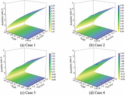
To investigate the influence of α_safe and α_service on the comprehensive system reliability result, the changes of comprehensive system reliability index β with different combinations of α_safe and α_service are investigated in this case, where α_safe is changed from 0.4 to 1.0 and α_service is changed from 1.0 to 2.0. The changes of β with α_safe and α_service for cases 1–4 are plotted in Figure 6(a) -(d), with the contours plotted for explicit illustration. It is found that:

1. For all the cases considered, the comprehensive reliability index β has increasing tendency with the increase of α_safe and α_service. This is because the value of comprehensive system LSF becomes larger with the increase of α_safe and α_service.

2. The increasing speed of β is more significant with the increase of α_safe than that with α_service, which is because the LSFs corresponding to the modified serviceability failure modes are relatively small and dominant the value of comprehensive system LSF. However, the influence of α_safe on β still cannot be neglected, as shown in Table 3.

3. When α_safe and α_service is close to 1 (i.e., α_safe≥0.5 and α_service≤1.5), the changing of β with these modified coefficients is relatively significant. When α_safe and α_service are far from 1 (i.e., α_safe<0.5 and α_service>1.5), β remains nearly no change with the increase of these coefficients. This is because the values of individual LSFs will become large with the large values of α_safe and α_service, the corresponding individual failure modes become too difficult to happen and thus have nearly no influence on the system reliability.

Figure 6. Changes of comprehensive reliability index β with α_safe and α_service for cases 1–4.

4.3. Comparison of system reliabilities corresponding to different limit states

To investigate the necessary of conducting comprehensive system reliability, the system reliability indices corresponding to different limit states are compared in this section. Five limit states are considered, which include comprehensive, ultimate, modified ultimate, serviceable, and modified serviceable limit states. The comprehensive system LSF is given in Eq. (33(33) $G_{sys}(\mathbf{X})=min[G_{M{U}_1}(\mathbf{X}),G_{M{U}_2}(\mathbf{X}),G_{M{U}_3}(\mathbf{X}),G_{M{U}_4}(\mathbf{X}),G_{M{U}_5}(\mathbf{X}),G_{M{S}_1}(\mathbf{X}),G_{M{S}_2}(\mathbf{X}),G_{M{S}_3}(\mathbf{X})]$(33) ), and the system LSFs corresponding to other limit states are formulated as follows:

Ultimate limit state:

(34a) $G_{U\mathrm{\_}sys}(\mathbf{X})=min[G_{U1}(\mathbf{X}),G_{U2}(\mathbf{X}),G_{U3}(\mathbf{X}),G_{U4}(\mathbf{X}),G_{U5}(\mathbf{X})]$(34a)

Modified ultimate limit state:

(34b) $G_{MU\mathrm{\_}sys}(\mathbf{X})=min[G_{M{U}_1}(\mathbf{X}),G_{M{U}_2}(\mathbf{X}),G_{M{U}_3}(\mathbf{X}),G_{M{U}_4}(\mathbf{X}),G_{M{U}_5}(\mathbf{X})]$(34b)

Serviceable limit state:

(34c) $G_{S\mathrm{\_}sys}(\mathbf{X})=min[G_{S1}(\mathbf{X}),G_{S2}(\mathbf{X}),G_{S3}(\mathbf{X})]$(34c)

Modified serviceable limit state:

(34d) $G_{MS\mathrm{\_}sys}(\mathbf{X})=min[G_{M{S}_1}(\mathbf{X}),G_{M{S}_2}(\mathbf{X}),G_{M{S}_3}(\mathbf{X})]$(34d)

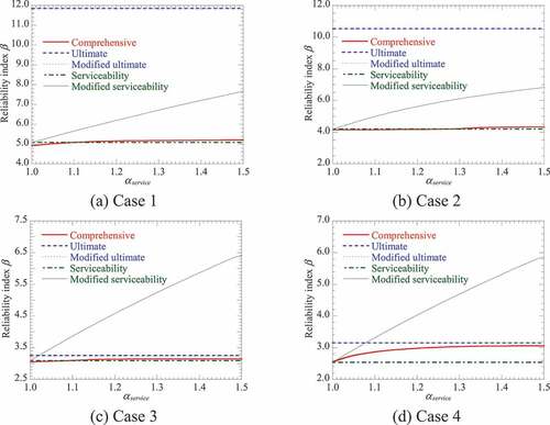
For an overall analysis, both the serviceability- and safety-dominant comprehensive system limit states are considered. When serviceability is dominant, α_service is 1, and the changes of reliability indices β with α_safe for cases 1–4 are, respectively, plotted in Figure 7(a) -(d). When safety is dominant, α_safe becomes 1, and the changes of reliability indices β with α_service for cases 1–4 are respectively plotted in Figure 8(a) -(d). The target reliability indices corresponding to the ultimate and serviceability limit states are 2.0 and 3.2, respectively (Liu et al. 2017). For comprehensive limit state, the target reliability index is approximately set to be that corresponding to the dominant limit state, i.e., the target reliabilities are, respectively, 2.0 and 3.2 for serviceability-and safety-dominant comprehensive limit states. It can be observed that:

1. When serviceability is dominant, β corresponding to the ultimate, serviceability, modified serviceability limit states remain the same with the change of α_safe, which is because the corresponding system LSFs have no relationship with α_safe. β corresponding to the modified safety limit state increases with the increase of α_safe, which indicates that the modified ultimate limit state becomes harder to be overcome with the increase of α_safe. As α_safe = C_service/C_safe is inversely proportional to the difference between the expected costs of the serviceability and ultimate limit states, the serviceability-dominant comprehensive system reliability is inversely proportional to the difference between C_service and C_safe.

2. When safety is dominant, β corresponding to the safety, serviceability, modified ultimate limit states remain the same with the change of α_service, which is because the corresponding system LSF have no relationship with α_service. β corresponding to the modified serviceability limit state increases with the increase of α_service, which indicates that the modified ultimate limit state becomes harder to be overcome with the increase of α_service. As α_service = C_safe/C_service is proportional to the difference between C_service and C_safe, the safety-dominant comprehensive system reliability is directly proportional to the difference between C_service and C_safe.

3. The reliability index β corresponding to ultimate limit state is always larger than that for serviceability limit state. This is because the expected cost of safe failure modes is much higher than those of serviceable failure modes, and thus, the ultimate limit state is defined to have a higher target reliability level. The results obtained by method of moments are consistent with the practice, which verifies the accuracy of the method of moments in conducting comprehensive system reliability analysis.

4. There is a significant difference between the comprehensive system reliability and the general system reliability indices, which consider the safety and serviceability separately. The general system reliability index of CRTS II track slab is always larger than the target reliability index. In contrast, when considering the serviceability-dominant comprehensive limit state, the comprehensive reliability index may be lower than the target value. It is indicated that, no maintenance will be performed based on general system reliability analysis results, which will endanger the quality or even safety of CRTS II track slab. Therefore, comprehensive system reliability analysis is necessary for the safety operation of CRTS II track slab.

Figure 7. Changes of β with α_safe corresponding to different limit states for α_service = 1.

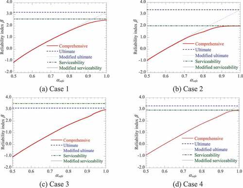
Figure 8. Changes of β with α_service corresponding to different limit states for α_safe = 1.

5. Conclusion

For an appropriate evaluation, the comprehensive system reliability considering safety and serviceability simultaneously is defined. A comprehensive system LSF model is proposed, and the procedure of comprehensive reliability analysis is developed by integrating method of moments with FE analysis. The comprehensive system LSF of CRTS II track slab is constructed considering important safety and serviceability failure modes. With the aid of the proposed method, the comprehensive system reliability of CRTS II track slab is analyzed, and the result is compared with that of general system reliability analysis considering safety and serviceability separately. It is found that:

1. The proposed comprehensive system LSF model has an explicit and flexible form. Comprehensive system reliability can be efficiently calculated by using method of moments combined with the proposed comprehensive model.

2. The comprehensive system reliability of CRTS II track slab is at a relatively high level, while the safety-dominant comprehensive system reliability is higher than the serviceability-dominant one. The difference in the expected costs for breaking the ultimate and serviceability limit states have significant influence on the comprehensive system reliability, which is inversely and directly proportional to the serviceability- and safety-dominant comprehensive system reliability, respectively.

3. There is significant difference among the comprehensive system reliability index of CRTS II track slab and the general system reliability indices. The general system reliability indices are always larger than the target value, while the comprehensive system reliability index may be lower than the target one. This indicates that the general system reliability analysis may overestimate the reliability level, and result in inappropriate decision on maintenance strategy. Thus, it is necessary to conduct comprehensive system reliability analysis for making appropriate maintenance strategy and ensuring the safety operation of a structure.

Acknowledgments

The study is partially supported by the National Natural Science Foundation of China (Grant Nos. 52108104, 51820105014, 51738001, and U19342171), the 111 Project (Grant No. D21001) and Science and Technology Research and Development Program Project of China Railway Group Limited (Major Special Project No. 2020-Special-02). The supports are gratefully acknowledged.

Disclosure statement

No potential conflict of interest was reported by the author(s).

Additional information

Notes on contributors

Xuan-Yi Zhang

Xuan-Yi Zhang is currently a lecturer of Beijing University of Technology. She got a PhD from Central South University, China. Her research interests mainly focuses on structural reliability.

Zhao-Hui Lu

Zhao-Hui Lu is currently a professor at Beijing University of Technology and former professor at Central South University, China. His expertise includes structural reliability and time-dependent reliability based risk-cost optimised maintenance strategy.

Yan-Gang Zhao

Yan-Gang Zhao is currently a professor at Kanagawa University, Japan and a guest professor at Beijing University of Technology, China. His research interest mainly focuses on structural reliability and seismic performance of engineering structures

Appendix A

Finite element model of CRTS II slab-type ballastless track system

Table 4. Material properties of the FE model of CRTS II slab-type ballastless track system.

Section	Element	Type	Value
Rail	BEAM 188	Elastic modulus (GPa)	210
		Poisson’s ratio	0.3
		Area (cm^2)	77.45
		Density (kg/m^3)	7800
Fastener	COMBIN 14	Stiffness (kN/m)	5 × 10^4
		Spacing (m)	0.65
CRTS II track slab	SHELL 63	Elastic modulus (GPa)	35.5
		Poisson’s ratio	0.2
		Length×width×thickness (m)	6.45 × 2.55 × 0.2
		Density (kg/m^3)	2500
CA mortar layer	COMBIN 14	Elastic modulus (GPa)	7
		Poisson’s ratio	0.2
		thickness (m)	0.03
		Density (kg/m^3)	1800
Foundation plate	SHELL 63	Elastic modulus (GPa)	30
		Poisson’s ratio	0.2
		Width×thickness (m)	2.95 × 0.2
		Density (kg/m^3)	2500
Viaduct girder	COMBIN 14	Equivalent elastic modulus (GPa/m)	1

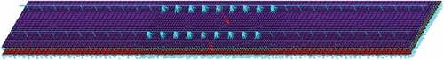
The FE model of CRTS II slab-type ballastless track system is constructed by ANSYS Finite Element Program, using the beam-plate model on elastic foundation. In order to eliminate the influence of boundary conditions, three continuous track slab model is used for the calculation as shown in Figure 9, and the middle track slab is selected as the research object.

Figure 9. FE model of CRTS II slab-type ballastless track system (Zhang et al. 2021).

The beam element is employed to model the rail, the shell element is used to model the track slab and foundation plate, and the strings element is employed to model the fasteners, CA mortar layer, and the viaduct girder. The input material properties of the elements are summarized in Table 4. Since the group wheel effect is smaller than the single wheel effect, the single axle model is adopted to represent the train load. For the analysis of the middle slab, the train loads are applied on fasteners in the middle of the rails with the value of α_pP_j, where P_j represents the static wheel load, and α_p =3.0 is the dynamic load factor of P_j for maximum train speed larger than 300kN/m (Ministry of Railways of the PRC. 2016).

References

- Chun, J., J. Song, and G. H. Paulino. 2015. “Parameter Sensitivity of System Reliability Using Sequential Compounding Method.” Structural Safety 55: 26–36. doi:10.1016/j.strusafe.2015.02.001.
- Cornell, C. A. 1976. “Bounds on the Reliability of Structural Systems.” Journal of Structural Division 93 (1): 171–200. doi:10.1061/JSDEAG.0001577.
- Ding, J., and X. Z. Chen. 2016. “Moment-based Translation Model for Hardening non-Gaussian Response Processes.” Journal of Engineering Mechanics 142 (2): 06015006. doi:10.1061/(ASCE)EM.1943-7889.0000986.
- Fleishman, A. L. 1978. “A Method for Simulating Non-normal Distributions.” Psychometrika 43 (4): 521–532. doi:10.1007/BF02293811.
- Gong, C. Q., and W. Zhou. 2017. “Improvement of Equivalent Component Approach for Reliability Analyses of Series Systems.” Structural Safety 68: 65–72. doi:10.1016/j.strusafe.2017.06.001.
- Hohenbichler, M., and R. Rackwitz. 1981. “Non-normal Dependent Vectors in Structural Safety.” Journal of Engineering Mechanics Division 107 (6): 1227–1238. doi:10.1243/03093247V164251.
- Li, H. Y., Z. W. Yu, J. F. Mao, and L. Z. Jiang. 2020a. “Nonlinear Random Seismic Analysis of 3D High-speed Railway Track-bridge System Based on OpenSEES.” Structures 24: 87–98. doi:10.1016/j.istruc.2020.01.003.
- Li, J., J. B. Chen, and W. L. Fan. 2007. “The Equivalent Extreme-value Event and Evaluation of the Structural System Reliability.” Structural Safety 29 (2): 112–131. doi:10.1016/j.strusafe.2006.03.002.
- Li, Y., J. J. Chen, J. X. Wang, X. F. Shi, and L. Chen. 2020. “Study on the Interface Damage of CRTS II Slab Track under Temperature Load.” Structures 26: 224–236. doi:10.1016/j.istruc.2020.04.014.
- Liu, X. Y., C. G. Su, D. Liu, F. Xiang, C. Gong, and P. R. Zhao. 2017. “Research on the Bond Properties between Slab and CA Mortar and the Parameters Study of Cohesive Model.” Journal of Railway Eng Ineering Soc Icence. 3(222):in Chinese. 22–28.
- Melchers, R. E. 1994. “Structural System Reliability Assessment Using Directional Simulation.” Structural Safety 16 (1–2): 23–37. doi:10.1016/0167-4730(94)00026-M.
- MRPRC, . 2016b. Provisional Code for Limit State Design Method of Railway Track: Q/CR 9130-2015,. Beijing, China: Ministry of Railways of the PRC.
- MRPRC, . 2016. Code for Design of High Speed Railway: TB10621-2014,. Beijing, China: Ministry of Railways of the PRC.
- NSPRC. 2018. Code for Design of Concrete Structures, GB 50010-2018. Beijing, China: Building Industry Publishing House.
- Ou, Z. M. 2016. “Fatigue reliability analysis methods and application for slab track structure.” PhD dissertation. Southeast University 123–134. (in Chinese)
- Song, J., and W. H. Kang. 2009. “System Reliability and Sensitivity under Statistical Dependence by Matrix-based System Reliability Method.” Structural Safety 31 (2): 148–156. doi:10.1016/j.strusafe.2008.06.012.
- Tong, M. N., Y. G. Zhao, Z. H. Lu, and Z. W. Yu. 2020. “Reliability Evaluation of Crack Width of CRTS II Ballastless Track Slab Using Methods of Moment.” Journal of the China Railway Society. 142(11):in Chinese. 130–138.
- Xu, H., and S. Rahman. 2004. “A Generalized Dimension-reduction Method for Multidimensional Integration in Stochastic Mechanics.” International Journal for Numerical Methods in Engineering 61 (12): 1992–2019. doi:10.1002/nme.1135.
- Yu, Z. W., and J. F. Mao. 2017. “Probability Analysis of Train-track-bridge Interactions Using a Random Wheel/rail Contact Model.” Engineering Structures 144: 120–138. doi:10.1016/j.engstruct.2017.04.038.
- Zhang, G. H. 2014. “Durability study on CRTS II type ballastless track slab based on reliability.” MA dissertation. Lanzhou Jiaotong University. (in Chinese)
- Zhang, X. Y., Z. H. Lu, Y. G. Zhao, and C. Q. Li. 2021. “Reliability Analysis of CRTS II Track Slab considering Multiple Failure Modes.” Engineering Structures 228: 111557. doi:10.1016/j.engstruct.2020.111557.
- Zhao, Y. G., and Z. H. Lu. 2021. Structural Reliability: Approaches from Perspectives. of statistical moments. Hoboken, NJ, USA: Wiley-Blackwell.
- Zhao, Y.-G., X.-Y. Zhang, and Z.-H. Lu. 2018. “Complete Monotonic Expression of the Fourth-moment Normal Transformation for Structural Reliability.” Computers and Structures 196: 186–199. doi:10.1016/j.compstruc.2017.11.006.