The economic value of urban landscapes in a suburban city of Tokyo, Japan: A semantic segmentation approach using Google Street View images

ABSTRACT

Visual impression of urban landscape has been investigated in detail through behavioral experiments and questionnaire surveys in the field of architecture. However, in order to give an incentive to build and maintain a good residential environment, an economic consideration of the urban landscape across space is also an important aspect. Employing a semantic segmentation approach using Google Street View images, we investigate the relationship between urban landscapes and property prices in low-rise residential areas in a suburban city of Tokyo, Japan. Such visual images are used to represent the landscape of both surrounding districts in general and the street-level landscape; more specifically, the latter is derived after controlling for the district fixed effect. We first show that greenery, openness and visual enclosure are positively correlated with property price at street level. We also investigate the value of urban landscapes commonly seen in Japan: (i) the presence of a power pole is negatively correlated with property price at district level; and (ii) the presence of a road shoulder or farmland, either of which may disrupt the continuity of a residential area, does not exhibit negative correlations with property price at either district or street level.

KEYWORDS:

• Hedonic price model
• landscape
• machine learning
• Google Street View images
• Japan

1. Introduction

Visual impression of urban landscape has been widely investigated in detail through behavioral experiments and questionnaire surveys in the field of architecture. Urban landscape impressions are basically based on components related to greenery, openness, and visual enclosure (e.g., Hirate and Yasuoka 1986; Ishikawa et al. 1995; Nishio and Ito 2015, 2020; Takei and Fukushima 1983). The other elements such as power poles (electrical wires) also form the urban landscape impression (Oku 1985). These urban landscapes may be recognized as a street level landscape or as a landscape having a certain spatial unit such as a district (Koura and Kamino 1995, 1996). However, whether these impressions are reflected in economic valuation has been less intensively investigated. In order to give an incentive to build and maintain a good residential environment, an economic consideration of the urban landscape across space is also an important aspect.

The quality of surrounding landscapes has a potential impact on real estate price formation because landscapes represent elements that make up the quality of the surrounding neighborhood. There are many factors forming property prices, including building characteristics (e.g., property age and floor area), land characteristics (e.g., land area and walking time to nearest station), and land use around the properties. The hedonic regression analysis separates the contribution of each component to property prices. The economic value of a landscape is captured using a landscape index, which provides additional explanatory variables to the basic characteristics. The landscape index has traditionally been created through a field survey, whereby criteria are set and scored by a researcher (Gao and Asami 2007). Alternatively, researchers collect detailed land use information (Gao and Asami 2001), advertising information or 3D geographical information on whether a property offers a scenic view, such as of the ocean (Jim and Chen 2009; Yamagata et al. 2016), to create the landscape index.

This paper further extends these methods by capturing urban landscape factors using Google Street View images. Recent research has recognized that by combining Street View images and artificial intelligence (AI) technology for image recognition, there is the potential to greatly improve urban landscape analyses (Biljecki and Ito 2021). Yang et al. (2021) have quantified the amount of greenery in Street View images based on the percentage of pixels recognized as greenery in the image. Using open-source image segmentation methods that employ deep learning (e.g., SegNet), recent studies have decomposed Street View images into each landscape element and have created indexes typically based on the pixel ratio (Chen et al. 2020; Fu et al. 2019; Ito and Biljecki 2021; Tang and Long 2019; Ye et al. 2019a, 2019b; Zhang and Dong 2018). Using these new approaches, recent literature investigates the relationship between property price and landscape elements, while the landscape type has been largely restricted to the proportions of greenery, sky and buildings present (Chen et al. 2020; Fu et al. 2019; Yang et al. 2021; Ye et al. 2019a; Zhang and Dong 2018). In Western contexts, other factors like “curb appeal” (that is, the attractiveness of the exterior of a property when viewed from a public space, such as a street or sidewalk), architectural style, and urban design elements have been gradually investigated using new image recognition technologies (Johnson, Tidwell, and Villupuram 2020; Lindenthal and Johnson 2021).

Greenery, openness, and visual enclosure are basic elements of urban landscapes in Japan and in other countries as well. However, other elements of urban landscapes differ greatly in Japan from those in Europe, the United States and even other Asian countries. Specifically, the existence of power poles above the ground, the presence of urban farmland within residential areas, and private parking space facing the road, are landscape factors specific to Japan that can be tested from the Street View image data. First, the undergrounding of power lines is not at all common in Japanese cities. Whereas major cities in Europe (such as London and Paris) and Asia (for instance, Hong Kong and Singapore) have all become pole-free, Japan lags behind, this goal being achieved in only 8% of Tokyo’s wards area and 6% of the city of Osaka.¹ The existence of power poles at ground level in residential areas potentially lowers the value of properties, as the overhead-to-underground conversion of electricity distribution networks has been perceived positively in Western countries, based on stated preferences (McNair et al. 2011; Tempesta, Vecchiato, and Girardi 2014).

Second, farmland remains within residential areas on the fringes of Japanese cities. Whereas in Western cities, urban planning concepts, such as zoning and greenbelt additions, have been applied to encourage controlled urban growth, Asian cities have historically placed land use patterns of urban and rural character next to each other (Yokohari et al. 2000). Although this type of landscape potentially gives us a positive impression through the provision of rural environments for urban residents, the presence of farmland may disrupt the continuity of an urban residential area; its specific impact is one of the issues examined in this paper. Third, unlike the parking space on road shoulders seen in Western cities, private parking space facing the road – that is, paved parking space within a private lot – is a typical characteristic of Japanese cities. Given that residential lots tend to be small in Japanese cities, a typical parking space is not hidden by fences or greenery (as will be shown in Section 4) and disrupts the continuity of a residential area. Intuitively the presence of such a car park would have a negative impact on neighboring property prices, but as this situation is common in Japan, its specific impact is one of the issues examined in this paper.

Figure 1. Methodological flow.

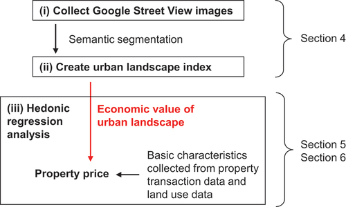
In low-rise residential areas in a suburban city of Tokyo, this paper investigates the relationship between common Japanese urban landscape and property prices via the following three steps. First, we collect Google Street View images in front of detached houses that have been sold. Second, we extract components of the landscape using AI technology for image recognition, and create what we call the “urban landscape index.” Specifically, we apply the recent semantic segmentation approach proposed by Tao, Sapra, and Catanzaro (2020), which as of August 2021 has achieved state-of-the-art results in two commonly used, large-scale open data sets: Mapillary and Cityscapes. This approach is impressive in its segmentation accuracy and label diversity compared to previous studies. Third, we construct a model to explain the extent to which these components contribute to the transaction price. After controlling for a sufficient range of characteristics of the properties and the neighborhoods considered, the strength of the correlation between the urban landscape index and property price is derived from the “landscape” channel. The component captured here as the urban landscape index may represent the landscape of the surrounding district in general (e.g., the landscape of a well-developed residence), or the street-level landscape more specifically. Thus, the landscape channel is distinguished as district-level and street-level, the latter of which is derived after further controlling for the district fixed effect.

The rest of the paper is organized as follows. Section 2 describes the study area and property transaction data. Section 3 presents the methodology. Section 4 presents examples of semantic segmentation of the Japanese landscape and develops hypotheses. Section 5 presents the variables and summary statistics for the following hedonic regression analysis. Section 6 shows the empirical results. Section 7 concludes the paper.

2. Study area and property transaction data

To investigate the economic value of urban landscape in typical low-rise residential areas commonly seen in the suburbs of metropolitan areas in Japan, the analysis is conducted in Hachioji city, a suburban city of Tokyo’s metropolitan area. The city is located more than 30 km away from Shinjuku Station, a terminus in central Tokyo. The population is around 577,000 according to the 2015 Census and has remained almost stable since 2005, and a relatively stable housing demand is expected in the analysis period. We employ samples in areas with designated zoning (that is, we exclude mountainous areas in which zoning is not applied), especially focusing on low-rise residential areas (i.e., category I, exclusively low-rise residential zones) in the main analysis. In our transaction samples of detached houses, 61% are located in low-rise residential areas.

We employ the transaction data of detached houses collected by an association of real estate agents through the Real Estate Information Network System (REINS).² Information on real estate transactions is recorded in these data, in the same way as in the Multiple Listing Service (MLS) in the United States. The REINS is the only real estate transaction system designated by the Ministry of Land, Infrastructure, Transport and Tourism (MLIT) in Japan, and is a representative system for real estate companies to register transaction information. The registration of data is considered to have sufficient coverage, as it is mandatory for a real estate agent or company to register the information on transacted properties under exclusive brokerage service agreement, although not for all properties. Indeed, transaction volumes in each regional submarket (mainly at prefecture level) based on the REINS data have been announced to the public as market reports.³ In this context, the number of samples and their property characteristics studied in this paper is likely to be representative of the submarket of Hachioji city.⁴

We employ newly built and resold detached houses transacted from 2016 to 2019. There are 800 observations in total in the low-rise residential areas considered (and 1,307 samples in the entire area of the Hachioji city), after truncating samples with missing or atypical information.⁵ The addresses are geocoded using Geocoding API, provided by Google. The transaction prices and other property characteristics (which will be shown later in Table 1(a) are recorded in the data. As we describe in the next section, variables constructed from the Google Street View images will be linked to the property transaction data.

Table 1. Summary statistics.

(a) Property characteristics
	Mean			S.D.
Dependent variable
Price [10,000 JPY]	2466.3			1115.9
Building characteristics
Newly built	0.250
Age [years]	17.5			14.4
Floor area [m^2]	107.3			27.9
Non-timbered	0.109
Land characteristics
Land area [m^2]	169.1			63.2
Walking time to station [min]	5.9			7.4
Bus to station	0.530
With parking space	0.755
Distance to junior high school [km]	0.777			0.401
Floor-area ratio (FAR) [%]	75.638			13.823
Front road width
Less than 4 m	0.034
4–5 m	0.179
5–6 m	0.196
6–7 m	0.254
7–10 m	0.053
10 m or more	0.093
Unknown	0.193
Land use within 500 m radius [ratio]
High-rise building	0.020			0.038
Dense low-rise building	0.021			0.081
Low-rise building	0.630			0.168
Vacant land	0.016			0.030
Park and green	0.005			0.014
Farmland	0.035			0.057
Number of observations	800
(b) Urban landscape index created through sematic segmentation of the Google Street View images
Variable	Mean		Min		Max
	Mean	S.D.	Mean	S.D.	Mean	S.D.
Vegetation	0.108	0.080			0.236	0.170
Sky	0.237	0.059			0.346	0.053
Building	0.200	0.088	0.068	0.059
Building + Wall + Fence	0.348	0.102
Pole	0.007	0.006			0.027	0.025
Sidewalk	0.029	0.023			0.094	0.057
Sidewalk + Car	0.042	0.030
Terrain	0.025	0.039			0.091	0.120

3. Methodology

Figure 1 shows the flow of our analyses. First, using Street View Static API, 12 Google Street View images (i.e., every 30 degrees) are collected in front of each transacted property. To be more specific, for each property, the nearest point on the road is chosen. Although the landscape impression may change depending on the retrieving point and on the angle, the effects are reduced when we take the average of the multiple images at the retrieving point. We collect the most recent images uploaded to Google Maps as of August 2021.

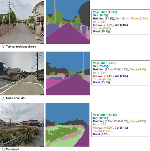
Figure 2. Examples of original images and semantic segmentation.The right-hand squares show the pixel ratios of each landscape component within the images.

Second, for the collected images, semantic segmentation is conducted, a deep learning algorithm that associates a label or category to every pixel in an image. We employ the recent semantic segmentation approach proposed by Tao, Sapra, and Catanzaro (2020), which as of August 2021 has achieved state-of-the-art results in two commonly used open data sets: Mapillary and Cityscapes. Cityscapes is a large data set that labels semantic classes across 5,000 urban street images in 50 German cities (Cordts et al. 2016). Mapillary Vistas is another large data set, containing 25,000 high-resolution images from across the world, with annotated semantic object categories (Neuhold et al. 2017). The semantic segmentation model is first pre-trained on the larger Mapillary, and then trained on Cityscapes. Using the pre-trained model, every Street View image is partitioned into multiple-segment categories: road, sidewalk, building, wall, fence, pole, traffic light, traffic sign, vegetation, terrain, sky, person, rider, car, truck, bus, train, motorcycle and bicycle. Given that some categories are almost blank, we create our urban landscape index using major categories (which are shown in Table 1(b)).

Third, we conduct hedonic regression analysis to decompose the property prices (that is, the sum of the building price and land price) into multiple components. There are many factors forming the property prices, including building characteristics (e.g., property age and floor area), land characteristics (e.g., land area and walking time to nearest station), and land use around the properties.⁶ Beyond these basic characteristics, this paper further extends these methods by capturing urban landscape factors using Google Street View images. It is expected that the urban landscape index would impact the land price, and the building price would be basically determined by the characteristics of building itself. Thus, we include the characteristics of building as explanatory variables in the hedonic regression analysis so that the building price level is sufficiently controlled.

We estimate the correlation between property price and urban landscape in the following regression:

(1) $ln{P}_{it}=\alpha +\hspace{0.17em}\sum _s{\beta }_s{V}_{si}^{\hspace{0.17em}}+\hspace{0.17em}\sum _k{\gamma }_k{X}_{ki}+D_j+T_t+e_{it}$(1)

where ln P_it is the log of the transaction price for unit i in period t. α is the constant. V_si is the urban landscape index for landscape component s, and β_s is the corresponding coefficient. Specifically, the index represents the proportion of landscape component s in the images, and is created through semantic segmentation of the Google Street View images. More precisely, 1% increase in the proportion of component s leads to a β_s% increase in the transaction price. X_ki is the control variable k shown in Table 1(a), and γ_k is the corresponding coefficient. D_j captures the district fixed effect, that is, it takes 1 for properties in district j, and 0 otherwise. T_t captures the quarterly fixed effect for the time of the transaction, that is, it takes 1 for a property transaction in period t, and 0 otherwise. e_it is the error term.

When we exclude the district fixed effect, D_j, the urban landscape index V_si serves as a proxy for the district-level landscape. For instance, if the entire residential area (i.e., the district) has been uniformly developed as a “greenery residential area,” the greenery is likely to be the district-level landscape. On the other hand, when we include the district fixed effect, D_j, the urban landscape index V_si serves as a proxy for the street-level landscape. For instance, even within each “greenery residential area” (i.e., within each district), openness can vary across streets.

4. Semantic segmentation and hypotheses development

4.1. Example of semantic segmentation

To ensure that each category from the semantic segmentation captures the intended landscape component, Figure 2 shows examples of original images and their semantic segmentation outcomes, as well as the pixel ratios of each landscape component within the images. Although the pre-trained model is trained on street images from all around the world, we confirm that the semantic segmentation is conducted properly for the Japanese Street View images.

Panel (a) shows a typical residential area. The dark green category captures vertical “greenery” as the vegetation component (accounting for 11.6% of the pixels in the entire image), including trees and plants. The blue category captures “openness” as the sky component (accounting for 28.3%). The dark gray category captures “visual enclosure” as the building component (accounting for 13.8%). In some cases, buildings are also captured by a wall (light blue category; accounting for 9.4%) or a fence (light pink category; accounting for 4.5%); thus, we will also create an alternative indicator of the visual enclosure as the sum of these three categories. The light gray category captures “power pole” as the pole component (accounting for 1.5%). The purple category captures the road component (accounting for 29.3%), and this is set as a reference category in the following hedonic regression analyses.

Panel (b) shows a case capturing “road shoulder,” which is an open space in the shoulder of a road that is often used as private parking space or as paved vacant lots.⁷ This is captured by the dark pink category as the sidewalk component (accounting for 6.1%). In some cases, cars are parked in the parking space, and so we will also create an alternative indicator of the road shoulder as the sum of the two components: sidewalk and car (dark blue category; accounting for 0.6%). Panel (c) shows a case capturing “farmland” within a residential area, which is the exposure of the ground. This is captured by the light green category as the terrain component (accounting for 16.9%). Note that the vertical greenery in the farmland is captured by the vegetation component.

For the typical residential area (panel (a) of Figure 2), Figure 3 shows 12 Street View images (i.e., every 30 degrees). Table 2 shows the proportion of each landscape component for these 12 views in percentage terms; the mean, minimum and maximum values for these 12 views are also calculated. Although the semantic segmentation is conducted properly overall, we see that there are some misclassifications of sidewalks, walls and fences by buildings (e.g., image number 5). It is also true that the proportion of buildings increases when the building is in the foreground (e.g., image number 10). These problems can be reduced by taking the mean value of the proportion for each component from the 12 views, justified by the fact that the landscape is an average impression from a 360-degree view at the location. The minimum or maximum values of the proportion from the 12 views may also be useful in capturing the strongest impression in the location. For instance, if the minimum proportion of the building is large, the impression conveyed is that the visual enclosure is high at the location; by contrast, the maximum proportion of the building may not be useful, because the view in front of the building is always included in the 12 views. Similarly, if the maximum proportion of vegetation is large, the impression conveyed is that the location has plenty of greenery.

Figure 3. 12 views (every 30 degrees) for the typical residential areas shown in Figure 2(a).

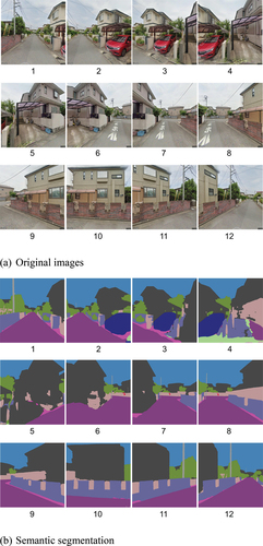
Table 2. Percentage of each landscape component for the 12 views of the typical residential areas shown in Figure 2(a).

Number	Vegetation	Sky	Building	Building + Wall + Fence	Pole	Sidewalk	Sidewalk + Car	Terrain
1	11.64	28.21	13.79	27.72	1.52	1.60	1.60	0.02
2	8.21	28.97	18.60	22.39	0.11	2.03	13.57	0.61
3	8.68	22.79	37.28	46.83	0.00	3.60	11.02	0.13
4	3.91	14.91	32.74	56.26	0.00	0.12	11.02	9.30
5	6.93	12.58	63.58	69.44	0.00	1.19	1.19	0.07
6	2.80	16.42	39.39	45.55	0.24	0.00	0.00	0.00
7	2.89	26.12	31.07	39.09	0.16	1.15	1.15	0.00
8	3.51	26.35	17.30	38.31	0.33	1.31	1.31	0.00
9	0.75	16.91	33.18	58.58	0.00	2.29	2.29	0.00
10	2.51	7.66	45.78	74.20	0.00	0.16	0.16	0.00
11	9.47	12.92	33.16	55.71	1.55	0.55	0.55	0.00
12	8.78	26.48	20.04	33.53	1.17	0.82	0.82	0.04
Mean	5.84	20.03	32.16	47.30	0.42	1.24	3.72	0.85
Min	0.75	7.66	13.79	22.39	0.00	0.00	0.00	0.00
Max	11.64	28.97	63.58	74.20	1.55	3.60	13.57	9.30

In the hedonic regression analysis, aggregated proportions of the 12 views (shown in bold) are employed.

4.2. Hypotheses

Based on the examples discussed above, Table 3 presents the hypotheses for the hedonic regression analysis. For each landscape element addressed here, we present the baseline and additional components of the images, the summary statistics to be measured, and a hypothesis on the direction of the correlation with the price level.

Table 3. Hypotheses regarding correlations between the urban landscape index and property price.

Landscape element	Urban landscape index	Summary statistics	Expected correlation with property price
Greenery	Vegetation	Mean (Max)	+ (Comfortable environment with abundant greenery and plantings)
Openness	Sky	Mean (Max)	+ (Sufficient sunlight in the community)
Visual enclosure	Building (+ Wall + Fence)	Mean (Min)	+ (Matured residential area with a certain level of enclosure by buildings)
Power pole	Pole	Mean (Max)	‐ (Messy Landscape characterized by electrical wires) or 0 (Common urban landscape in Japan)
Road shoulder	Sidewalk (+ Car)	Mean (Max)	? (Loss of continuity of buildings or visual enclosures; Enhance openness; Common urban landscape in Japan)
Farmland	Terrain	Mean (Max)	? (Loss of continuity of buildings or visual enclosures; Enhance openness; Common urban landscape in Japan)

Our hypotheses on the major scene perceptions are basically consistent with previous studies on the visual impression of urban landscape in the field of architecture (e.g., Hirate and Yasuoka 1986; Ishikawa et al. 1995; Nishio and Ito 2015, 2020; Takei and Fukushima 1983) and on the relationship between property price and landscape elements using recent image recognition technologies (e.g., Chen et al. 2020; Fu et al. 2019; Yang et al. 2021; Ye et al. 2019a; Zhang and Dong 2018). “Greenery” is captured through the mean or maximum proportion of the vegetation component. It is expected to have a positive relationship with transaction price through the provision of a comfortable environment with abundant greenery and plantings. “Openness” is captured through the mean or maximum proportion of the sky component. It is expected to have a positive relationship with transaction price by offering sufficient sunlight to the community. “Visual enclosure” is captured through the mean or minimum proportion of the building component, as well as the mean proportion of the sum of the building, wall and fence components. Sufficient level of visual enclosure represents that the residential area is matured, and thus, it is expected to have a positive relationship with transaction price.

With regard to urban landscapes specific to Japan, “power pole” is captured through the mean or maximum proportion of the pole component. It is expected to have a nonpositive relationship with transaction price, as it is a messy landscape characterized by electrical wires in the sky, but it is so common in the Japanese landscape that it may not reduce the transaction price. “Road shoulder” is captured through the mean or maximum proportion of pixels for the sidewalk component, as well as the mean proportion of the sum of the sidewalk and car components. Its relationship with transaction price is unclear; although it reduces the continuity of buildings or the visual enclosure, it enhances the openness. This is so common in the Japanese landscape that it may not reduce the transaction price. “Farmland” is captured through the mean or maximum proportion of the terrain component. Its relationship with transaction price is also unclear; the same mechanisms as for road shoulder apply.

5. Variables and summary statistics

We employ low-rise residential area samples for the main analysis. Table 1 shows summary statistics (means and standard deviations) for (a) property characteristics and (b) urban landscape index, the latter of which is created through sematic segmentation of the Google Street View images. In panel (a), the building characteristics include: a newly built dummy (taking 1 for a newly built house and 0 otherwise); property age; floor area; and a non-timbered dummy (most Japanese detached houses are timbered). The land characteristics include: land area; walking time to the nearest station; a dummy variable indicating a need to take a bus to the nearest station; a dummy variable for a lot with parking space; distance to a junior high school; and the regulation (upper limit) of the floor-area ratio (FAR). After controlling for the existence of parking space in the lot, the road shoulder captures the landscape of the location. Front road width is included as a categorical variable. In Japan, if the front road width is less than 4 m (and the length of the lots connected to the road is less than 2 m), rebuilding the existing house is forbidden. The “less than 4 m category” is expected to be negatively correlated with price. The unknown status is included so as not to delete missing observation samples, which exist in non-negligible numbers.

Land use within a 500 m radius around the property (that is, the ratio of each land use type) is measured using a geographic information system (GIS) based on 50 m-mesh land use data, provided as National Land Information (Ministry of Land, Infrastructure, Transport and Tourism). The categories include: high-rise building; dense low-rise building (that is, a low-rise building is densely concentrated in the area); low-rise building (the most common surrounding land use type, as we employ low-rise residential area samples); vacant land; park and green space (well-maintained park or green space); and farmland. After controlling for the initial three categories, “openness” and “visual enclosure” capture the landscape of the location. Further, the last three categories control part of the quality of the location. The existence of vacant land partly controls for the sidewalk component, the existence of a park and/or green space partly controls for the vegetation component (and even the pole component, as the overall quality of the location), and the existence of farmland around the location partly controls for the farmland component.

In panel (b), the means and standard deviations of the urban landscape index created through sematic segmentation of the Google Street View images are shown for the mean and minimum and maximum proportions. On average, vegetation, sky and buildings account for 10.8%, 23.7%, and 20.0%, respectively, of the mean proportion. On the other hand, the corresponding values for pole, sidewalk and terrain are less than 5%. As expected, the average of the minimum (maximum) proportion is smaller (larger) than the mean proportion of the corresponding landscape component; these variables will be employed in the robustness checks.

6. Empirical results

6.1. Main results

Table 4 shows the correlation between property price and the urban landscape index based on equation (1)(1) $ln{P}_{it}=\alpha +\hspace{0.17em}\sum _s{\beta }_s{V}_{si}^{\hspace{0.17em}}+\hspace{0.17em}\sum _k{\gamma }_k{X}_{ki}+D_j+T_t+e_{it}$(1) . As in the following discussion, the results confirm that the quality of surrounding landscapes has a meaningful relationship with real estate price formation following the hypotheses in Table 2. Columns (1) and (2) control only the very basic variables, and thus the urban landscape index simply serves as a locational proxy. Columns (3) and (4) add control variables, but still do not include the district fixed effect, hence column (4) measures the district-level landscape. Columns (5) and (6) now include the district fixed effect, and thus column (6) measures the street-level landscape. Comparing R² between columns (1) and (2) (0.635 and 0.652), between columns (3) and (4) (0.695 and 0.705), and between columns (5) and (6) (0.794 and 0.801), reveals that the landscape index partly improves the explanatory power of the model. However, the degree of improvement is much larger when we include additional control variables.

Table 4. Correlations between urban landscape index and property price.

Measuring:		Locational proxy		District-level landscape		Street-level landscape
		(1)	(2)	(3)	(4)	(5)	(6)
Urban landscape index
Vegetation (Mean)			0.6469***		0.5866***		0.3454*
			(0.1924)		(0.1892)		(0.2018)
Sky (Mean)			0.9836***		0.9684***		1.0541***
			(0.2866)		(0.2957)		(0.2905)
Building (Mean)			0.2578		0.2528		0.5360***
			(0.1743)		(0.1750)		(0.1980)
Pole (Mean)			−3.6017*		−3.4615*		−1.2807
			(1.9449)		(1.7929)		(1.8650)
Sidewalk (Mean)			1.3820***		0.7494		0.1757
			(0.5338)		(0.5243)		(0.5769)
Terrain (Mean)			−0.4643		−0.2295		−0.0182
			(0.3085)		(0.2788)		(0.2567)
Building characteristics
Newly built		0.0114	0.0111	0.0644*	0.0578	0.1072***	0.1038***
		(0.0337)	(0.0351)	(0.0350)	(0.0360)	(0.0346)	(0.0345)
Age [years]		−0.0180***	−0.0180***	−0.0169***	−0.0170***	−0.0169***	−0.0167***
		(0.0013)	(0.0013)	(0.0013)	(0.0013)	(0.0013)	(0.0012)
Floor area [m^2]		0.0064***	0.0063***	0.0051***	0.0050***	0.0041***	0.0041***
		(0.0007)	(0.0007)	(0.0007)	(0.0007)	(0.0007)	(0.0007)
Non-timbered				0.0384	0.0395	0.0415	0.0437
				(0.0418)	(0.0413)	(0.0413)	(0.0408)
Land characteristics
Land area [m^2]		0.0019***	0.0017***	0.0019***	0.0018***	0.0017***	0.0016***
		(0.0004)	(0.0004)	(0.0004)	(0.0004)	(0.0004)	(0.0004)
Walking time to station [min]		−0.0130***	−0.0139***	−0.0157***	−0.0162***	−0.0098***	−0.0095***
		(0.0028)	(0.0027)	(0.0030)	(0.0030)	(0.0037)	(0.0035)
Bus to station		−0.5044***	−0.5210***	−0.4926***	−0.5077***	−0.2076***	−0.2138***
		(0.0396)	(0.0389)	(0.0449)	(0.0459)	(0.0792)	(0.0751)
With parking space				0.0474*	0.0462*	0.0462*	0.0491*
				(0.0280)	(0.0280)	(0.0254)	(0.0250)
Distance to junior high school [km]				−0.1268***	−0.1238***	−0.0099	−0.0238
				(0.0277)	(0.0278)	(0.0558)	(0.0544)
Floor-area ratio (FAR) [%]				−0.0010	−0.0011	0.0018*	0.0015
				(0.0008)	(0.0008)	(0.0010)	(0.0009)
Front road width
Less than 4 m				−0.1234**	−0.1421***	−0.1656***	−0.1651***
				(0.0515)	(0.0549)	(0.0546)	(0.0581)
4–5 m				−0.1595***	−0.1614***	−0.1363***	−0.1430***
				(0.0350)	(0.0355)	(0.0340)	(0.0345)
5–6 m				(reference)	(reference)	(reference)	(reference)
6–7 m				0.0433	0.0344	−0.0213	−0.0265
				(0.0280)	(0.0277)	(0.0291)	(0.0285)
7–10 m				0.0352	0.0099	0.0082	−0.0062
				(0.0481)	(0.0469)	(0.0492)	(0.0475)
10 m or more				0.0217	−0.0091	−0.0276	−0.0394
				(0.0487)	(0.0482)	(0.0488)	(0.0456)
Unknown				−0.0357	−0.0370	−0.0606*	−0.0579*
				(0.0343)	(0.0340)	(0.0337)	(0.0328)
Land use within 500 m radius [ratio]
High-rise building				0.3648	0.2703	0.3789	0.1972
				(0.2777)	(0.2817)	(0.5165)	(0.5177)
Dense low-rise building				0.4992***	0.5111***	0.5392*	0.2361
				(0.1279)	(0.1322)	(0.2855)	(0.2908)
Low-rise building				0.1109	0.0854	0.1773	0.1054
				(0.0789)	(0.0844)	(0.1200)	(0.1198)
Vacant land				0.9247***	0.7879***	0.1512	−0.0726
				(0.3043)	(0.2929)	(0.5705)	(0.5676)
Park and green				2.9514***	2.3671***	−1.0923	−1.3626
				(0.7220)	(0.7411)	(1.0142)	(1.0067)
Farmland				−0.2368	−0.3831**	0.0651	−0.0975
				(0.1917)	(0.1836)	(0.2975)	(0.2872)
Constant		7.3556***	7.0257***	7.5285***	7.2457***	7.2960***	6.9458***
		(0.0799)	(0.1387)	(0.1272)	(0.1528)	(0.1989)	(0.2100)
Time fixed effect (quarterly)		Yes	Yes	Yes	Yes	Yes	Yes
District fixed effect						Yes	Yes
Number of observations		800	800	800	800	800	800
R^2		0.635	0.652	0.695	0.705	0.794	0.801
Adjusted R^2		0.624	0.638	0.678	0.687	0.751	0.757

The dependent variable is the log of the transaction price. White-corrected robust standard errors are in parentheses. Significance level: *** p < 0.01, ** p < 0.05, * p < 0.1.

First, greenery, openness, and visual enclosure are positively correlated with property price at street level. In column (6) including the district fixed effect, the coefficients of the mean proportions of vegetation, sky, and building are positive with statistical significance. A 1% increase in the proportion of vegetation, sky, and building, respectively, lead to 0.34%, 1.05%, and 0.53% increases in transaction price.

The coefficient of vegetation is larger when we use much fewer control variables, showing that greenery partly serves as a locational proxy. Specifically, the park and green space ratio within 500 m is positive and statistically significant in column (4); this and the other control variables explain the decrease in the size of the coefficient for the mean proportion of the vegetation component from column (2) to column (4). However, greenery still captures the street-level landscape; that is, even within a district, the level of greenery is different on each street. Specifically, the coefficient of vegetation is still positive with 10% statistical significance in column (6), which controls for the district fixed effect.⁸ This is in contrast to the fact that the park and green space ratio within 500 m now becomes negative without statistical significance; the effect of the existence of a well-maintained park or green space, which is likely to capture the characteristics of the district, is absorbed by the district fixed effect.

The coefficient of sky does not vary much even when we control much fewer control variables in columns (2) and (4), demonstrating that openness is heterogeneous across districts and across the streets within a district. The coefficient of building diminishes and loses statistical significance once we control for much fewer control variables in columns (2) and (4). This shows that visual enclosure is heterogeneous across the streets within a district, but does not have a clear trend across districts.

Second, the presence of a power pole is negatively correlated with property price at district level. In column (4) without controlling for the district fixed effect, the coefficient of pole is negative with statistical significance; a 1% increase in the proportion of pole leads to a 3.46% decrease in transaction price. However, once we control for the district fixed effect in column (6), the size of the coefficient diminishes and statistical significance is lost. This shows that power poles serve as a district-level landscape. The negative valuation at district-level means that it is recognized as a messy landscape characterized by electrical wires in the sky, and that the residential area achieving high valuation is likely to have less power poles in the whole district.

Let us roughly discuss the size of the coefficient of the pole component at district level, 3.46. Three power poles are recognized in the semantic segmentation in the typical residential area in Figure 2(a), and this is summarized as a mean proportion of 0.42% in Table 1. Thus, one power pole lowers property prices by (3.46 × 0.42)/3 = 0.48 [%], compared to a pole-free landscape. Given that each power pole lowers non-negligible numbers of surrounding houses, the overhead-to-underground conversion of electricity distribution networks is likely to improve property values widely in the residential area.

Third, the presence of either a road shoulder or farmland does not exhibit negative correlations with property price even at district level. In both columns (4) and (6), the coefficients of sidewalk are positive but without statistical significance. The coefficient becomes larger as fewer control variables are included; thus, the sidewalk component partly serves as a proxy of locational quality. In both columns (4) and (6), the coefficients of terrain are negative but without statistical significance. The coefficient becomes larger in absolute terms as fewer control variables are included; thus, the terrain component partly serves as a proxy of locational quality. The insignificant or neutral valuations of road shoulder and farmland mean that these types of landscape have two sides: They reduce the continuity of buildings or the visual enclosure, while they enhance the openness. It is also true that the landscapes are so common in Japanese residential areas that they may not be reflected in the valuations.

With regard to the control variables, a narrow front road width (less than 5 m) reduces property price with statistical significance. Most of the land use ratio within 500 m radius of a transacted property exhibits statistical significance when we do not control for the district fixed effect (column (4)). However, it loses statistical significance once we control for the district fixed effect (column (6)). This confirms that the district fixed effect control is effective in accounting for the heterogeneity in land use across districts.

6.2. Subsample on land use type

Table 5 shows the entire area sample (columns (1) and (2)) and subsamples of other residential areas (excluding residential areas with a category I exclusively low-rise residential zone; columns (3) and (4)) and loosely regulated areas (quasi-industrial zones, neighborhood commercial zones, and commercial zones; columns (5) and (6)). Columns (1), (3) and (5) capture the district-level landscape without controlling for the district fixed effect (corresponding to column (4) of Table 4), while columns (2), (4) and (6) capture the street-level landscape by controlling for the district fixed effect (corresponding to column (6) of Table 4). The nonexclusive zoning system used in Japan restricts specific types of land use in a location, and does not intend to realize a single (pure) land use therein. “Low-rise residential area” is the strictest type of zoning, literally allowing only low-rise residential houses to be situated in an area. In an “other residential area,” low-rise and high-rise residential houses (and even other facilities) can coexist. In a “loosely regulated area,” residential houses and commercial/industrial uses can coexist. In this context, the economic value of landscape is more likely to be observed in pure low-rise residential areas, and may be lost in more loosely regulated areas where multiple types of land use coexist.

Table 5. Subsample analysis of land use type.

Sample:		Entire area		Other residential area		Loosely regulated area
Measuring:		District-level landscape	Street-level landscape	District-level landscape	Street-level landscape	District-level landscape	Street-level landscape
		(1)	(2)	(3)	(4)	(5)	(6)
Urban landscape index
	Vegetation (Mean)	0.4505***	0.1060	0.2889	0.1646	0.1436	−0.0573
		(0.1582)	(0.1695)	(0.3808)	(0.4132)	(0.5192)	(0.6095)
	Sky (Mean)	0.6148***	0.7087***	0.3485	0.4885	0.0111	0.4896
		(0.2009)	(0.2046)	(0.4133)	(0.5209)	(0.5656)	(0.8693)
	Building (Mean)	0.1893	0.3214**	−0.0310	0.5410	0.3167	0.3383
		(0.1392)	(0.1497)	(0.3956)	(0.4030)	(0.3864)	(0.5824)
	Pole (Mean)	−1.5049	0.0444	1.6424	7.8979	2.9837	3.9114
		(1.3403)	(1.5129)	(3.5051)	(5.9158)	(2.6071)	(4.2802)
	Sidewalk (Mean)	0.3459	−0.0141	−0.1771	1.6259	−0.3943	−1.2080
		(0.4646)	(0.4866)	(0.9767)	(1.2077)	(1.2012)	(1.8886)
	Terrain (Mean)	−0.4776*	−0.1830	−0.8464**	0.1083	−0.6307	−0.6099
		(0.2498)	(0.2389)	(0.4156)	(0.4695)	(0.5149)	(0.9942)
Building characteristics, Land characteristics, Land use within 500 m radius, Zoning category, Time fixed effect (quarterly) and a Constant		Yes	Yes	Yes	Yes	Yes	Yes
District fixed effect			Yes		Yes		Yes
Number of observations		1307	1307	297	297	210	210
R^2		0.699	0.795	0.742	0.894	0.756	0.875
Adjusted R^2		0.686	0.757	0.693	0.806	0.684	0.748

The dependent variable is the log of the transaction price. White-corrected robust standard errors are in parentheses. Significance level: *** p < 0.01, ** p < 0.05, * p < 0.1.

In columns (1) and (2), the entire area sample basically confirms the same results as those yielded from our main analysis using low-rise residential areas (Table 4), except for the loss of statistical significance for the vegetation component at street level. This may be due to the fact that the other residential area and loosely regulated area subsamples do not show a correlation between vegetation and property price (columns (3)–(6)). In other words, street-level greenery is evaluated only within low-rise residential areas. Note that terrain exhibits a negative correlation with property price at district level. This may capture the strong heterogeneity across districts when we employ the entire sample. That is, areas with farmland may have been facing housing development only recently, and thus still retain low land prices.

In the other residential areas (columns (3) and (4)) and in loosely regulated areas (columns (5) and (6)), we do not observe a correlation between the urban landscape index and transaction price with statistical significance (except that terrain exhibits a negative correlation with property price at district level in other residential areas, as in the entire area). This implies that the urban landscape is basically reflected in transaction price only in low-rise residential areas, in which the landscape is valued by market participants. In the remaining areas, other factors like transportation and shopping convenience matter, whereas the urban landscape does not influence the transaction price.

6.3. Robustness checks

Table 6 conducts robustness checks by using alternative indicators of the urban landscape index. The samples are properties in low-rise residential areas, as in Table 4. Columns (1), (3), (5) and (7) capture the district-level landscape without controlling for the district fixed effect (corresponding to column (4) of Table 4), while columns (2), (4), (6) and (8) capture the street-level landscape by controlling for the district fixed effect (corresponding to column (6) of Table 4). We employ alternative indicators one by one, and the other baseline indicators are included as control variables. For instance, when we employ the maximum proportion of vegetation (instead of the mean proportion of vegetation), we include the mean proportions of sky, building, pole, sidewalk, and terrain. The results are basically consistent with those presented in Table 4.

Table 6. Robustness checks.

(a) Greenery, openness and visual enclosure
Measuring:		District-level landscape	Street-level landscape	District-level landscape	Street-level landscape	District-level landscape	Street-level landscape	District-level landscape	Street-level landscape
		(1)	(2)	(3)	(4)	(5)	(6)	(7)	(8)
Urban landscape index
Alternative indicator
	Vegetation (Max)	0.2312***	0.1781**
		(0.0842)	(0.0886)
	Sky (Max)			0.6096**	0.7201***
				(0.2603)	(0.2541)
	Building (Min)					0.3150	0.6047**
						(0.2181)	(0.2417)
	Building + Wall + Fence (Mean)							0.1377	−0.1104
								(0.2400)	(0.2400)
Baseline indicator
	Vegetation (Mean)			0.3657**	0.1219	0.5445***	0.2394	0.5503**	−0.0936
				(0.1728)	(0.1735)	(0.1727)	(0.1798)	(0.2614)	(0.2682)
	Sky (Mean)	0.8598***	1.0606***			0.8706***	0.8275***	0.9398**	0.4881
		(0.2905)	(0.2782)			(0.2695)	(0.2515)	(0.3971)	(0.3722)
	Building (Mean)	0.1612	0.5294***	0.0390	0.3121*
		(0.1663)	(0.1850)	(0.1556)	(0.1615)
	Pole (Mean)	−3.6499**	−1.2459	−3.1002*	−0.9070	−3.7286**	−2.0014	−3.4045*	−1.7044
		(1.7957)	(1.8669)	(1.7543)	(1.8524)	(1.8196)	(1.9027)	(1.7803)	(1.8727)
	Sidewalk (Mean)	0.7678	0.1951	0.9873*	0.4614	0.7256	0.1422	0.9189*	0.1610
		(0.5217)	(0.5753)	(0.5092)	(0.5609)	(0.5280)	(0.5842)	(0.5239)	(0.5981)
	Terrain (Mean)	−0.2364	−0.0334	−0.2364	−0.0302	−0.1958	0.0276	−0.1925	−0.1518
		(0.2756)	(0.2545)	(0.2780)	(0.2637)	(0.2894)	(0.2712)	(0.2981)	(0.2826)
Building characteristics, Land characteristics, Land use within 500 m radius, Time fixed effect (quarterly) and a Constant		Yes	Yes	Yes	Yes	Yes	Yes	Yes	Yes
District fixed effect			Yes		Yes		Yes		Yes
Number of observations		800	800	800	800	800	800	800	800
R^2		0.705	0.801	0.702	0.798	0.705	0.800	0.704	0.798
Adjusted R^2		0.686	0.758	0.683	0.754	0.687	0.756	0.686	0.753
(b) Power pole, road shoulder, and farmland
Measuring:		District-level landscape	Street-level landscape	District-level landscape	Street-level landscape	District-level landscape	Street-level landscape	District-level landscape	Street-level landscape
		(1)	(2)	(3)	(4)	(5)	(6)	(7)	(8)
Urban landscape index
Alternative indicator
	Pole (Max)	−0.7583*	−0.3847
		(0.4217)	(0.4510)
	Sidewalk (Max)			0.1081	0.0442
				(0.1977)	(0.2030)
	Sidewalk + Car (Mean)					0.5241	0.2099
						(0.3816)	(0.3497)
	Terrain (Max)							−0.0931	0.0017
								(0.0954)	(0.0906)
Baseline indicator
	Vegetation (Mean)	0.5967***	0.3453*	0.5783***	0.3434*	0.5965***	0.3532*	0.6010***	0.3439*
		(0.1890)	(0.2019)	(0.1896)	(0.2017)	(0.1893)	(0.2009)	(0.1911)	(0.2038)
	Sky (Mean)	0.9552***	1.0531***	0.9987***	1.0584***	0.9716***	1.0473***	0.9759***	1.0524***
		(0.2928)	(0.2890)	(0.2903)	(0.2874)	(0.2941)	(0.2852)	(0.2945)	(0.2903)
	Building (Mean)	0.2565	0.5360***	0.2601	0.5369***	0.2413	0.5285***	0.2530	0.5372***
		(0.1747)	(0.1980)	(0.1751)	(0.1987)	(0.1757)	(0.1992)	(0.1746)	(0.1981)
	Pole (Mean)			−3.6663**	−1.2998	−3.5458**	−1.2658	−3.3911*	−1.2803
				(1.7483)	(1.8453)	(1.7694)	(1.8492)	(1.7998)	(1.8701)
	Sidewalk (Mean)	0.7509	0.1687					0.7269	0.1860
		(0.5234)	(0.5776)					(0.5198)	(0.5726)
	Terrain (Mean)	−0.2359	−0.0189	−0.3090	−0.0290	−0.2540	−0.0110
		(0.2783)	(0.2567)	(0.2780)	(0.2575)	(0.2784)	(0.2635)
Building characteristics, Land characteristics, Land use within 500 m radius, Time fixed effect (quarterly) and a Constant		Yes	Yes	Yes	Yes	Yes	Yes	Yes	Yes
District fixed effect			Yes		Yes		Yes		Yes
Number of observations		800	800	800	800	800	800	800	800
R^2		0.705	0.801	0.704	0.801	0.705	0.801	0.705	0.801
Adjusted R^2		0.686	0.757	0.686	0.757	0.686	0.757	0.687	0.757

The dependent variable is the log of the transaction price. White-corrected robust standard errors are in parentheses. Significance level: *** p < 0.01, ** p < 0.05, * p < 0.1.

Panel (a) presents the results regarding greenery, openness, and visual enclosure. In columns (1) and (2), we employ the maximum proportion of the vegetation component, whose coefficient is positive with statistical significance at street level. Thus, we confirm the robustness on the fact that greenery is positively correlated with property price at street level. Columns (3) and (4) employ the maximum proportion of the sky component, whose coefficient is positive with statistical significance at street level. Thus, we confirm the robustness of the fact that openness is positively correlated with property price at street level. Columns (5) and (6) employ the minimum proportion of the building component, whose coefficient is positive with statistical significance at street level. Thus, we confirm the robustness of the fact that visual enclosure is positively correlated with property price at street level. Note, however, that the mean proportion of the sum of the three components (building, wall, and fence) does not exhibit a correlation with transaction price in columns (7) and (8). This implies that the building component – but not the wall or fence components – is correlated with property price.

Panel (b) displays the results for power pole, road shoulder, and farmland. In columns (1) and (2), we employ the maximum proportion of the pole component, whose coefficient is negative with statistical significance only at district level. Thus, we confirm the robustness of the fact that the presence of a power pole is negatively correlated with property price at district level. In columns (3) and (4) (columns (5) and (6)), we employ the maximum proportion of the sidewalk component (mean proportion of the sum of the sidewalk and the car components). In neither regression are the coefficients statistically significant, confirming the robustness of the fact that the presence of a road shoulder does not exhibit a negative correlation with property price at either district or street level. In columns (7) and (8), we employ the maximum proportion of the terrain component. The coefficients are not statistically significant, confirming the robustness of the fact that the presence of farmland does not exhibit a negative correlation with property price at either district or street level.

7. Conclusion

While visual impression of urban landscape has been investigated in detail in the field of architecture, an economic consideration of the urban landscape across space is also an important aspect to give an incentive to build and maintain a good residential environment. Employing a novel semantic segmentation approach using Google Street View images, we have investigated the relationship between urban landscapes and property prices in low-rise residential areas in a suburban city of Tokyo, Japan. Such visual images have been used to represent the landscape of both surrounding districts in general and the street-level landscape; more specifically, the latter has been derived after controlling for the district fixed effect. We first showed that greenery, openness and visual enclosure are positively correlated with property price at street level. We then investigated the value of common Japanese urban landscapes: (i) the presence of a power pole is negatively correlated with property price at district level; and (ii) the presence of a road shoulder and farmland, either of which may disrupt the continuity of a residential area, does not exhibit negative correlations with property price at either district or street level. Thus, the quality of surrounding landscapes, as captured through Street View images, has a meaningful relationship with real estate price formation.

Our results suggest that basic landscape elements, such as greenery, openness and visual enclosure, are important in maintaining the value of residential areas; thus, protection of the residential environment through residential area planning and/or building agreement is meaningful. Furthermore, the value of residential areas can be increased by promoting the undergrounding of power poles. Although road shoulder does not lead to a uniform decline in economic value, the value of the landscape is potentially improved if it is well designed, such as a parking lot covered with greenery. Since farmland also does not lead to a uniform decline in economic value, preservation of urban farmland within residential area, in other words, coexistence of the two types of land use, may be justified.

Our results also show that the semantic segmentation approach, with high segmentation accuracy and label diversity, enables researchers to quantify micro-level landscapes that have previously proven difficult to obtain at large scale, and that this methodology is also useful in analyzing urban landscapes specific to Japan. The Hachioji city investigated in this paper is a typical low-rise residential area in the suburbs, and the conclusions of this study are likely to be a common feature of at least the suburban areas of major metropolitan areas.

Although the methodology is easily applicable to other types of real estate in different regions, subsample analysis of land use type indicates that any correlation between landscape and property price may be heterogeneous (e.g., central area and other suburban areas), and thus a functional form of hedonic regression should be tailored to each local context. To fulfill this aim, automating functional form to identify the elements that formulate property prices (e.g., He, Páez, and Liu 2017; Law, Paige, and Russell 2019; Law et al. 2020) is worthy of investigation.

Acknowledgments

We would like to thank two anonymous referees, Yasushi Asami, Masayoshi Hayashi, Sachio Muto, Toshihiko Yamasaki, Noriyuki Yanagawa, participants in the CREI workshop at the University of Tokyo, and members of Japan Real Estate Institute for their insightful comments. We also thank the Real Estate Information Network System (REINS) and Joint Research Program No. 1075 at the Center for Spatial Information Science, The University of Tokyo, for providing the data.

Disclosure statement

No potential conflict of interest was reported by the author(s).

Additional information

Funding

The authors gratefully acknowledge the support received from JSPS KAKENHI Grant Numbers 20K14896, 20H00082, and 17H00988, and a Google Cloud Platform Credit Coupon at The University of Tokyo.

Notes on contributors

Masatomo Suzuki

Masatomo Suzuki is a specially appointed associate professor at Center for the Promotion of Social Data Science Education and Research, Hitotsubashi University. His research interests include housing, real estate, city planning, and urban economics.

Junichiro Mori

Junichiro Mori is an associate professor at Graduate School of Information Science and Engineering, The University of Tokyo. His research interests include artificial intelligence, massive data analysis, and social network analysis.

Takashi Nicholas Maeda

Takashi Nicholas Maeda is an associate professor at the School of System Design and Technology of Tokyo Denki University. His research interests include causal discovery and urban computing.

Jun Ikeda

Jun Ikeda is a former graduate student at Graduate School of Information Science and Technology, The University of Tokyo.

Notes

¹ Ministry of Land, Infrastructure, Transport and Tourism. “Status of development of non-pole systems (domestic and overseas).” Available at: https://www.mlit.go.jp/road/road/traffic/chicyuka/chi_13_01.html (in Japanese; accessed 9 December 2021).

² For details, see: http://www.reins.or.jp/ (in Japanese; accessed 22 December 2021).

³ For details of the market data created from the REINS database, see: http://www.reins.or.jp/library/2019.html (accessed 16 February 2022; in Japanese).

⁴ Further, for condominiums in the Tokyo metropolitan area, Shimizu, Nishimura, and Watanabe (2016) compare the nature of the REINS data and other related data sources: properties listed in a web portal provided by one of the largest private vendors of residential information, and transacted properties (a part of registered properties) whose transaction prices are collected by the MLIT. It is shown that the regression coefficients in the hedonic regression analyses are at least consistent even though there may be differences in property characteristics.

⁵ In this low-rise residential area, we truncate 118 samples for inaccurate addresses, 26 samples for having a property age older than 50 years, and 27 samples for other missing information.

⁶ The economic value of urban landscape for existing properties can be captured through a property transaction price, which is the sum of building and land prices. The transaction price in our data more formally captures a market valuation than publicly available appraisals of land prices in Japan. Employing land transaction data also has difficulty in acquiring Google Street View images containing buildings that will be constructed on the land after the transactions; this may completely alter the landscape of newly developing residential areas.

⁷ It is true that in some cases, sidewalks are really sidewalks for wider streets. However, as in Figure 2(a), in typical residential districts with narrow streets, it is not common to see sidewalks with curbstones. Note that we controlled for the front road width in the hedonic regression analyses to partially separate this effect.

⁸ The variance inflation factor (VIF) for the urban landscape index in Table 4 (columns (1), (4), and (6)) is less than 5, not a level that would cause much of a multicollinearity problem. At variable level, the correlation between the “vegetation” and the “park and green space ratio” is weak (correlation coefficient of 0.03), implying that the greenery differs on each street, as a landscape.

References

- Biljecki, F., and K. Ito. 2021. “Street View Imagery in Urban Analytics and GIS: A Review.” Landscape and Urban Planning 215: 104217.
- Chen, L., X. Yao, Y. Liu, Y. Zhu, W. Chen, X. Zhao, and T. Chi. 2020. “Measuring Impacts of Urban Environmental Elements on Housing Prices Based on Multisource Data: A Case Study of Shanghai, China.” ISPRS International Journal of Geo-Information 9 (2): 106. doi:10.3390/ijgi9020106.
- Cordts, M., M. Omran, S. Ramos, T. Rehfeld, M. Enzweiler, R. Benenson, U. Franke, S. Roth, and B. Schiele. 2016. “The Cityscapes Dataset for Semantic Urban Scene Understanding.” In Proceedings of the IEEE Conference on Computer Vision and Pattern Recognition (CVPR), Las Vegas, NV, USA. 3213–3223.
- Fu, X., T. Jia, X. Zhang, S. Li, Y. Zhang, and S. Fu. 2019. “Do Street-Level Scene Perceptions Affect Housing Prices in Chinese Megacities? An Analysis Using Open Access Datasets and Deep Learning.” PloS ONE 14 (5): e0217505. doi:10.1371/journal.pone.0217505.
- Gao, X., and Y. Asami. 2001. “The External Effects of Local Attributes on Living Environment in Detached Residential Blocks in Tokyo.” Urban Studies 38 (3): 487–505. doi:10.1080/00420980120027465.
- Gao, X., and Y. Asami. 2007. “Effect of Urban Landscapes on Land Prices in Two Japanese Cities.” Landscape and Urban Planning 81 (1–2): 155–166. doi:10.1016/j.landurbplan.2006.11.007.
- He, L., A. Páez, and D. Liu. 2017. “Built Environment and Violent Crime: An Environmental Audit Approach Using Google Street View.” Computers, Environment and Urban Systems 66: 83–95. doi:10.1016/j.compenvurbsys.2017.08.001.
- Hirate, K., and M. Yasuoka. 1986. “A Study on the Evaluation of Street-Vistas with Roadside Trees: The Experiments with Using Black and White Photomontage Slidefilms.” Journal of Architecture, Planning and Environmental Engineering (Transactions of AIJ) 362: 35–43. [in Japanese]. doi:10.3130/aijax.362.0_35.
- Ishikawa, T., A. Okabe, Y. Sadahiro, and S. Kakumoto. 1995. “A Study on the Cognition of Open Space Using 3-D Stereo GIS.” Journal of Architecture and Planning (Transactions of AIJ) 475: 149–154. [in Japanese]. doi:10.3130/aija.60.149_5.
- Ito, K., and F. Biljecki. 2021. “Assessing Bikeability with Street View Imagery and Computer Vision.” Transportation Research Part C: Emerging Technologies 132: 103371. doi:10.1016/j.trc.2021.103371.
- Jim, C. Y., and W. Y. Chen. 2009. “Value of Scenic Views: Hedonic Assessment of Private Housing in Hong Kong.” Landscape and Urban Planning 91 (4): 226–234. doi:10.1016/j.landurbplan.2009.01.009.
- Johnson, E. B., A. Tidwell, and S. V. Villupuram. 2020. “Valuing Curb Appeal.” The Journal of Real Estate Finance and Economics 60 (1): 111–133. doi:10.1007/s11146-019-09713-z.
- Koura, H., and K. Kamino. 1995. “Study on Structure of Integrated Setting in Townscape of Urban Environment.” Journal of the City Planning Institute of Japan 30: 223–228. [in Japanese]. doi:10.11361/journalcpij.30.223.
- Koura, H., and K. Kamino. 1996. “Structure of Integrated Setting in Townscape as Pedestrian Environment.” Journal of Architecture and Planning (Transactions of AIJ) 484: 167–174. [in Japanese]. doi:10.3130/aija.61.167_3.
- Law, S., B. Paige, and C. Russell. 2019. “Take a Look Around: Using Street View and Satellite Images to Estimate House Prices.” ACM Transactions on Intelligent Systems and Technology (TIST) 10 (5): 1–19. doi:10.1145/3342240.
- Law, S., C. I. Seresinhe, Y. Shen, and M. Gutierrez-Roig. 2020. “Street-Frontage-Net: Urban Image Classification Using Deep Convolutional Neural Networks.” International Journal of Geographical Information Science 34 (4): 681–707. doi:10.1080/13658816.2018.1555832.
- Lindenthal, T., and E. B. Johnson. 2021. “Machine Learning, Architectural Styles and Property Values.” The Journal of Real Estate Finance and Economics. forthcoming. doi:10.1007/s11146-021-09845-1.
- McNair, B. J., J. Bennett, D. A. Hensher, and J. M. Rose. 2011. “Households’ Willingness to Pay for Overhead-to-underground Conversion of Electricity Distribution Networks.” Energy Policy 39 (5): 2560–2567. doi:10.1016/j.enpol.2011.02.023.
- Neuhold, G., T. Ollmann, S. Rota Bulò, and P. Kontschieder. 2017. “The Mapillary Vistas Dataset for Semantic Understanding of Street Scenes.” In Proceedings of the IEEE International Conference on Computer Vision (ICCV), Venice, Italy. 4990–4999.
- Nishio, S., and F. Ito. 2015. “The Effect of Sky Factor and the Change on Impression of Townscape: With the Experiment for Evaluation Impression while Walking.” Journal of Architecture and Planning (Transactions of AIJ) 710: 907–914. [in Japanese]. doi:10.3130/aija.80.907.
- Nishio, S., and F. Ito. 2020. “Statistical Validation of Utility of Head-mounted Display Projection-based Experimental Impression Evaluation for Sequential Streetscapes.” Environment and Planning B: Urban Analytics and City Science 47 (7): 1167–1183.
- Oku, T. 1985. “The Influence of Townscape Elements on the Estimation of Townscape: Experimental Study on Visual Characteristics and Feelings of Townscape Part 2.” Journal of Architecture, Planning and Environmental Engineering (Transactions of AIJ) 351: 27–37. [in Japanese]. doi:10.3130/aijax.351.0_27.
- Shimizu, C., K. G. Nishimura, and T. Watanabe. 2016. “House Prices at Different Stages of the Buying/Selling Process.” Regional Science and Urban Economics 59: 37–53. doi:10.1016/j.regsciurbeco.2016.04.001.
- Takei, M., and T. Fukushima. 1983. “A Study on Effect of Tree Planning Which Mitigates the Sense of Oppression by A Building: A Study on Visual Environmental Planning of Urban District.” Journal of Architecture and Planning (Transactions of AIJ) 332: 102–110. [in Japanese].
- Tang, J., and Y. Long. 2019. “Measuring Visual Quality of Street Space and Its Temporal Variation: Methodology and Its Application in the Hutong Area in Beijing.” Landscape and Urban Planning 191: 103436. doi:10.1016/j.landurbplan.2018.09.015.
- Tao, A., K. Sapra, and B. Catanzaro. 2020. “Hierarchical Multi-scale Attention for Semantic Segmentation.” arXiv preprint arXiv:2005.10821.
- Tempesta, T., D. Vecchiato, and P. Girardi. 2014. “The Landscape Benefits of the Burial of High Voltage Power Lines: A Study in Rural Areas of Italy.” Landscape and Urban Planning 126: 53–64. doi:10.1016/j.landurbplan.2014.03.003.
- Yamagata, Y., D. Murakami, T. Yoshida, H. Seya, and S. Kuroda. 2016. “Value of Urban Views in a Bay City: Hedonic Analysis with the Spatial Multilevel Additive Regression (SMAR) Model.” Landscape and Urban Planning 151: 89–102. doi:10.1016/j.landurbplan.2016.02.008.
- Yang, J., H. Rong, Y. Kang, F. Zhang, and A. Chegut. 2021. “The Financial Impact of Street-level Greenery on New York Commercial Buildings.” Landscape and Urban Planning 214: 104162. doi:10.1016/j.landurbplan.2021.104162.
- Ye, Y., H. Xie, J. Fang, H. Jiang, and D. Wang. 2019a. “Daily Accessed Street Greenery and Housing Price: Measuring Economic Performance of Human-scale Streetscapes via New Urban Data.” Sustainability 11 (6): 1741. doi:10.3390/su11061741.
- Ye, Y., W. Zeng, Q. Shen, X. Zhang, and Y. Lu. 2019b. “The Visual Quality of Streets: A Human-centred Continuous Measurement Based on Machine Learning Algorithms and Street View Images.” Environment and Planning B: Urban Analytics and City Science 46 (8): 1439–1457.
- Yokohari, M., K. Takeuchi, T. Watanabe, and S. Yokota. 2000. “Beyond Greenbelts and Zoning: A New Planning Concept for the Environment of Asian Mega-Cities.” Landscape and Urban Planning 47 (3–4): 159–171. doi:10.1016/S0169-2046(99)00084-5.
- Zhang, Y., and R. Dong. 2018. “Impacts of Street-visible Greenery on Housing Prices: Evidence from a Hedonic Price Model and a Massive Street View Image Dataset in Beijing.” ISPRS International Journal of Geo-Information 7 (3): 104. doi:10.3390/ijgi7030104.