Method of estimating the lateral vibration of an elevator rope from the vertical vibration of a compensating sheave

ABSTRACT

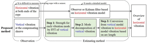
Observing the vibration of the elevator ropes in an elevator shaft is a difficult task. Although several methods of observing the displacement using image processing or laser displacement meters and then estimating the vibration through an observer or a Kalman filter have been developed, it is difficult to install sensors because of the movement of the elevator car and the thinness of the rope as an observation target. Therefore, in this study, we focus on a pulley called a compensating sheave that does not change its lateral position as the car and ropes move. The horizontal vibration of the ropes causes the compensating sheave to vibrate in the vertical direction. A method of estimating the horizontal vibration from this vertical vibration using arc length calculations and a short-time fast Fourier transform is proposed. First, the vertical vibration of the compensating sheave is distributed to the various mode responses based on the predominant frequency of the vertical vibration. The mode-decomposed vertical vibration is then converted into a horizontal mode response using an arc length relational expression. Analysis of seismic response data confirms that the proposed method can estimate the 1st, 2nd, and 3rd horizontal mode responses from the vertical vibration.

KEYWORDS:

• Elevator rope
• arc length
• compensating sheave
• vibration
• state estimation
• geometric relationship

1. Introduction

The continuing worldwide construction of high-rise buildings has heightened the importance of elevators as a means of vertical motion within buildings. As shown in Figure 1, elevator shafts contain a number of ropes – including the main ropes, compensation ropes, and various cables – that move in conjunction with the ascent or descent of the elevator car. Building vibrations during earthquakes may cause these ropes to undergo large-amplitude vibrations. In a high-rise building, the natural frequencies of the building are close to those of the elevator ropes in the low-order modes. Thus, the ropes resonate with the building and increase their amplitude. This is known as the problem of rope sway. Large rope-sway amplitudes may result in damage to hardware arising when ropes and cables collide with – or get caught on – protrusions within the shaft, such as rail brackets or mounting hardware used to affix equipment installations. Emergency control of elevators during earthquakes has been the subject of extensive research, which has demonstrated the effectiveness of control systems that use seismic early-warning systems to halt the motion of elevators before the arrival of the main shocks (Kubo et al. 2009). In previous work, we proposed a sway-control technique that – assuming elevator operation has been suspended by an emergency control system – seeks to accelerate the restoration of elevator functions with the minimum incurred damage by reducing the maximum response and shortening the duration of vibrations (e.g., (Miura and Kohiyama 2012; Nguyen, Miura, and Sone 2019)). Most of the vibration control is achieved through feedback control, so it is necessary to acquire a real-time vibration response. A common response estimation method for condition monitoring or feedback control involves an observer or a Kalman filter. If the real system can be modeled, it is possible to create an observer or a Kalman filter and estimate the state variables. The “horizontal” vibration model of the rope is generally a string model, which is solved by the finite difference method (Teshima et al. 2002), finite element method (Otsuki et al. 2006), or assumed-mode technique (Benosman 2014). That is, modeling is possible, and many studies have used observers and Kalman filters.

Figure 1. Ropes in an elevator shaft. The compensation rope connects the car and the counterweight on the lower side via the compensating sheave for balancing the mass.

However, observation problems remain. It is difficult to install sensors that stably observe the horizontal vibration of the rope. The first problem, mainly for the main rope and the compensation rope, is that the car travels up and down. When the sensor is installed on the elevator shaft, the observed position of the rope (whether it is an antinode or a node) changes as the car moves. If sensors are attached to the car or the sheave, only the responses at the ends of the rope can be obtained. The second problem is that the rope does not swing in a single axis and the diameter of the rope is relatively small. Thus, it may not pass through the laser emitted by the laser displacement meter. Takumi and Utsuno (Takumi and Utsuno 2022) have succeeded in measuring the amplitude at a position 0.5 m from the end of a 2-m rope by using a slit-type laser displacement meter. This method can observe “small” amplitude vibration.

To solve these problems, especially for compensation ropes, this paper focuses on the vertical vibration of the pulley, which is called the compensating sheave. There is a groove for the rope in the sheave, and the rope hangs in the groove. The protrusion from the compensating sheave slides on the guide (support) in the vertical direction, so the compensating sheave can vibrate freely along the vertical guide. Thus, it is easy to obtain the displacement and acceleration of the vertical vibration of the compensating sheave. As a result, it is not necessary to change the sensor position even when the car is moving, and it remains possible to observe the movement of the pulley when the rope vibration deviates slightly from the main vibration direction. However, the relation between “vertical” vibration and “horizontal” vibration has not been fully clarified. There are many studies dealing with rope vibrations. Takumi and Utsuno (Takumi and Utsuno 2022) evaluate damping using a rope with fixed length positions at both ends. In this case, the rope vibrates as it stretches. However, the vertical displacement of a sheave (or a car) had not been considered. Wu et al. (Shuiyuan, Ping, and Gong 2021) establish the mathematical model and mechanical model of the horizontal vibration of the steel wire rope. In their experiment, the mass block (car) on one end of the rope can move along a vertical guide. In this research, there is an assumption that the vibration of the mass block is ignored in the vertical direction. There are also studies using models that include both vertical and horizontal motion (Nguyen, Miura, and Sone 2019; Otsuki et al. 2006; Yang et al. 2017; Xiujuan, Zhanga, and Qin 2019), but vertical motion (car motion) is not affected by horizontal motion (rope). In addition, much research has been done that deals only with the vertical vibrations of elevator systems (Watanabe and Okawa 2018; Zhang et al. 2019; Hucheng, Zhang, and Cheng 2019; Peng et al. 2020). Zhang et al. (Zhang et al. 2019) model a main rope with a variable stiffness spring and analyze the vertical vibration of a high-speed elevator system as the car moves vertically. Evaluation of the physical parameters and analysis of the vertical vibration of the rope due to the vertical motion of the car are very valuable for elucidating complex elevator systems. However, the horizontal vibration of the rope and the vertical vibration of the sheave really have a mathematical or physical relationship. Watanabe (Watanabe 2020) proposed a model relating rope lateral vibration to vertical vibration via rope tension, with the rope vertical vibration related to the lateral vibration via the amount of pulling up caused by rope sway. In an experiment conducted by Ito et al. (Ito, Morishita, and Kimura 2006), the correlation between the horizontal displacement at the center of rope and the vertical displacement of mass was found to decrease when the rope vibrates at a frequency away from the first mode. This is probably because the observation point of the rope is a node in the secondary mode. Furthermore, the relation between the maximum horizontal displacement of the rope and the vertical displacement of the mass differs for each vibration mode. Analysis of the relationship contributes to easier estimation of the horizontal vibration of the rope.

This paper presents an estimation method that restores the modal responses instead of directly linking the vertical displacement of the compensating sheave to the horizontal displacement of the rope. An outline of the proposed method is shown in Figure 2. The novelty of this proposal is that it does not require a detailed model, unlike estimation based on a Kalman filter or an observer. Furthermore, it is difficult to obtain the displacement of the swaying rope with a sensor, but the proposed method measures the sheave moving on the guide, so measurement failure does not occur.

Figure 2. Estimation procedure.

The compensating sheave vibrates up and down as the ropes vibrate horizontally. The relation between vertical modal vibration and horizontal modal vibration is formulated over a reasonable range of amplitudes for rope vibration. This paper does not solve the coupled problem of horizontal motion and vertical motion, but obtains a geometric correlation based on the integral equation of arc length, which does not have a closed-form solution.

2. Materials and methods

Because the actual rope behavior includes the expansion and contraction of the rope and the vertical vibration of the car, the sheave also moves up and down during normal operation (Watanabe et al. 2013). In addition, the rope vibrations are so complex that some assumptions must be made. First, it is assumed that the rope vibration on the counterweight side can be suppressed by a vibration suppressor (Kimura 2016). As the vibration suppressor raises the natural frequency along with the physical restraint effect, it is considered that the rope is unlikely to resonate with the building response. Therefore, it does not become too large. Second, it is assumed that the friction between the sheave and the ropes prevents the rope on the counterweight side from moving to the car side via the compensating sheave. Therefore, the focus of this study is on the car side. Third, although there are multiple ropes, they are assumed to vibrate in approximately the same mode, so the ropes can be evaluated as a single rope. Relaxing these assumptions would require more detailed simulations or experimental verification.

2.1. Estimation theory

2.1.1. Relation between amplitude and arc length of sine function

To the best of the authors’ knowledge, Equation (1)(1) $l={\int }_{xmin}^{xmax}\sqrt{1+{\left(\frac{dy}{dx}\right)}^2}dx$(1) for the arc length l from x_min to x_max of a curve y = f(x), including simple curves, cannot be solved in most cases.

(1) $l={\int }_{xmin}^{xmax}\sqrt{1+{\left(\frac{dy}{dx}\right)}^2}dx$(1)

Therefore, the arc length from 0 to π of the sine function (2) with the amplitude a is calculated using Equation (3)(3) $l={\int }_0^{\pi }\sqrt{1+{\left(\frac{dy}{dx}\right)}^2}dx\approx \sum _{s=1}^m\sqrt{{\left(\frac{\pi }{m}\right)}^2+{\left\{f\left(\frac{\pi }{m}s\right)-f\left(\frac{\pi }{m}(s-1)\right)\right\}}^2},$(3) :

(2) $y=f(x)=asinx,$(2)

(3) $l={\int }_0^{\pi }\sqrt{1+{\left(\frac{dy}{dx}\right)}^2}dx\approx \sum _{s=1}^m\sqrt{{\left(\frac{\pi }{m}\right)}^2+{\left\{f\left(\frac{\pi }{m}s\right)-f\left(\frac{\pi }{m}(s-1)\right)\right\}}^2},$(3)

where m is the number of partitions and s is the element number. As an example, Figure 3 shows y and l when a = 1 and N = 10⁶π. When the amplitude a of the sinusoidal curve changes, the right end of the red line moves by l-π. The relation between the length l-π and the amplitude a is plotted in Figure 4. When a is in the range (0, 0.1], as shown in Figure 4(a), the approximate relation between a and l-π is as follows:

Figure 3. Sinusoidal curve y = a sin x ($0\le x\le \pi$) and its length l. When a straight line of length l bends in the shape of a sin x, the right edge moves to the left by l-π.

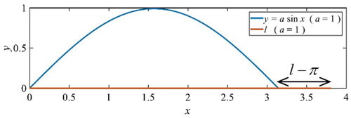
Figure 4. Applicable range of approximate curve. The relation between a and l-π differs depending on whether a is small or large. (a) (0, 0.1]; (b) (0, 10.0].

(4) $a=\sqrt{\frac{l-\pi }{0.7835}}$(4)

The approximation in Figure 4(a) provides a reasonable fit. Note that the approximation only holds when a is sufficiently small, as is clear from Figure 4(b), in which the range of a has been extended. Table 1 summarizes the ranges of amplitude a and the approximate quadratic functions with an intercept term of 0. When the range of a is large, the linear term becomes dominant over the square term. Now, the integration range is from 0 to π. Therefore, a = 3 means that the amplitude and the integration range are almost equal. In the relation between the rope amplitude and the sheave displacement discussed in the remainder of this paper, the deformed shape of a = 1 shown in Figure 3 is unrealistic. Therefore, l-π can be regarded as proportional to the square of a.

Table 1. Approximate curves.

Range of a (divided width of a is 0.001)	l-π
0.001 ~ 0.100	0.7835a^2 + 0.0001a
0.001 ~ 1.000	0.6326a^2 + 0.0573a
0.001 ~ 2.000	0.4310a^2 + 0.2356a
0.001 ~ 3.000	0.2993a^2 + 0.4298a

2.1.2. Rope vibration amplitude and end point movement

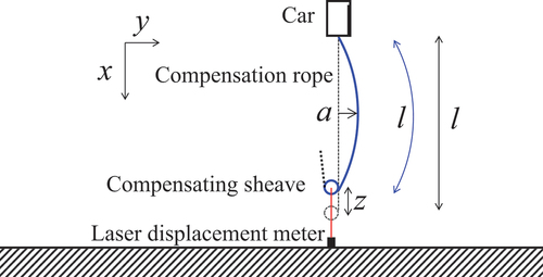
The compensation rope is now discussed in a similar manner as in Section 2.1. The vertical vibration of the compensating sheave z can be measured using a laser displacement meter positioned directly under the sheave. When the rope deforms, as shown in Figure 5, the rope length l satisfies the following equations:

Figure 5. Relation between vertical vibration of the compensating sheave z and horizontal vibration of the compensation rope a.

(5) $y=asin\frac{x}{l-z}\pi ,$(5)

(6) $l={\int }_0^{l-z}\sqrt{1+{\left(\frac{dy}{dx}\right)}^2}dx.$(6)

The result for l = 200 m is shown as the intersection of the curved surface and the plane in Figure 6, because Equations (5)(5) $y=asin\frac{x}{l-z}\pi ,$(5) and (6(6) $l={\int }_0^{l-z}\sqrt{1+{\left(\frac{dy}{dx}\right)}^2}dx.$(6) ) cannot be solved. According to the discussion in Section 2.1, the intersection curve can be estimated as a quadratic function.

Figure 6. Rope length l when the vertical displacement of the compensating sheave is z and the horizontal amplitude of the compensation rope is a. (b) is the view of (a) from the upper side of the l-axis.

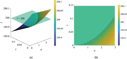
To express the intersection curve mathematically, the discretization steps of a and z are reduced: 0.01 for a and 0.001 for z. The value of z that gives the smallest absolute value of the difference from the plane for each value of a is then selected. The pairs of a and z are approximated by a quadratic equation with an intercept term of 0. Table 2 summarizes the rope length l and the approximate quadratic function.

Table 2. Approximate formulae of vertical displacement z. a varies from 0.005 to 2.495 in increments of 0.01. The coefficient of the first-order term increases when the rope length l becomes small.

l	z × 10^3
200	12.3a^2 + 0.0a
175	14.1a^2 + 0.0a
150	16.5a^2 – 0.0a
125	19.7a^2 + 0.0a
100	24.7a^2 – 0.0a
75	32.9a^2 + 0.1a
50	49.5a^2 – 0.1a
25	99.6a^2 – 0.9a

Assuming that the quadratic terms are dominant, they can be combined into one function of l and z as follows:

(7) $a=\sqrt{\frac{lz}{2.5}}$(7)

This is in good agreement with Watanabe’s result (Watanabe 2020),

(8) $z=\frac{{\pi }^2}{4l}{a}^2\approx \frac{2.5}{l}{a}^2,$(8)

which was calculated using terms up to the first order of the Taylor series for the integrand in Equation (6)(6) $l={\int }_0^{l-z}\sqrt{1+{\left(\frac{dy}{dx}\right)}^2}dx.$(6) .

In the case of the vibration shape in the N-th mode, represented by Equation (9)(9) $y=a_{N}sin\frac{Nx}{l-z_N}\pi$(9) , the influence of the amplitude a_N on the vertical displacement z_N is divided over the N modes. Thus, Equation (10)(10) $a_N=\frac{1}{N}\sqrt{\frac{l{z}_N}{2.5}}$(10) is obtained.

(9) $y=a_{N}sin\frac{Nx}{l-z_N}\pi$(9)

(10) $a_N=\frac{1}{N}\sqrt{\frac{l{z}_N}{2.5}}$(10)

The response z_N of each mode to z, shown in Figure 7, is explained in Section 2.3. Note that Equation (7)(7) $a=\sqrt{\frac{lz}{2.5}}$(7) is only an approximation of the quadratic term, or the approximate solution using only limited terms of the Taylor series. When the rope length l is too small or the order N is too large, the influence of the linear term in Table 2 becomes large, and the approximation may not be good. The limit at which Equation (10)(10) $a_N=\frac{1}{N}\sqrt{\frac{l{z}_N}{2.5}}$(10) can be applied is that if at least the first-order mode is predominant, l = 25 m is sufficient and the influence of the square term is dominant. Additionally, if l < 25 m, the amplitude a does not increase, so Equation (10)(10) $a_N=\frac{1}{N}\sqrt{\frac{l{z}_N}{2.5}}$(10) is sufficiently accurate.

Figure 7. Vertical vibration of the compensating sheave z_N and horizontal vibration of the compensation rope a_N for each mode. (a) 1st; (b) 2nd; (c) 3rd; (d) Combination of 1st to 3rd modes (a₁: a₂: a₃ = 5: 3: 2).

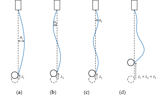
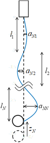
In the case of Figure 8, where the mode shape is not a uniform sine wave because of the influence of the rope’s own weight, among other factors, the vertical vibration z_N is expressed by the following equations as the sum of the contributions of the N elements:

Figure 8. Rope vibration when the tension distribution in the length direction is large.

(11) $z_N=\sum _{j=1}^N{z}_{Nj},\left(j=1,2,\dots ,N\right),$(11)

(12) $a_{Nj}\approx \sqrt{\frac{l_j{z}_{Nj}}{2.5}}$(12)

where Equation (12)(12) $a_{Nj}\approx \sqrt{\frac{l_j{z}_{Nj}}{2.5}}$(12) is derived from Equation (7)(7) $a=\sqrt{\frac{lz}{2.5}}$(7) . Substituting Equation (12)(12) $a_{Nj}\approx \sqrt{\frac{l_j{z}_{Nj}}{2.5}}$(12) into Equation (11)(11) $z_N=\sum _{j=1}^N{z}_{Nj},\left(j=1,2,\dots ,N\right),$(11) gives the following expression

(13) $z_N=\sum _{j=1}^N{z}_{Nj}\approx 2.5\sum _{j=1}^N\frac{{a_{Nj}}^2}{l_j}.$(13)

The variables representing average values are given by Equations (14)(14) ${\bar{a}}_N^2=\frac{\sum _{j=1}^N{a}_{Nj}^2}{N}$(14) and (15(15) ${\bar{l}}_N=\frac{\sum _{j=1}^N{l}_j}{N}=\frac{l}{N}$(15) ).

(14) ${\bar{a}}_N^2=\frac{\sum _{j=1}^N{a}_{Nj}^2}{N}$(14)

(15) ${\bar{l}}_N=\frac{\sum _{j=1}^N{l}_j}{N}=\frac{l}{N}$(15)

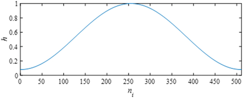
Using a linear density ρ, the tension S related to the length direction y and natural frequency f_i, the i-th mode shape ${\phi }_i$ is given by the following equation [11](11) $z_N=\sum _{j=1}^N{z}_{Nj},\left(j=1,2,\dots ,N\right),$(11) :

(16) ${\phi }_i=\frac{1}{{\left(\rho S(y)\right)}^{\frac{1}{4}}}sin\left\{2\pi f_i{\int }_0^y\sqrt{\frac{\rho }{S(y)}}dy\right\}.$(16)

For example, Figure 9 shows the tension distributions and mode shapes given by Equation (16)(16) ${\phi }_i=\frac{1}{{\left(\rho S(y)\right)}^{\frac{1}{4}}}sin\left\{2\pi f_i{\int }_0^y\sqrt{\frac{\rho }{S(y)}}dy\right\}.$(16) for various weights of the compensating sheave connected to a 200-m rope with ρ = 2.11 kg/m.

Figure 9. Rope tension distribution and mode shape distortion. (a) Rope tension distribution; (b) mode shape.

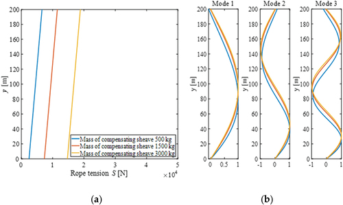
Figure 9 shows that if the mass of the sheave is more than about 1500 kg, the influence of the weight of the rope can be ignored. Therefore, Equations (14)(14) ${\bar{a}}_N^2=\frac{\sum _{j=1}^N{a}_{Nj}^2}{N}$(14) and (15(15) ${\bar{l}}_N=\frac{\sum _{j=1}^N{l}_j}{N}=\frac{l}{N}$(15) ) can be regarded as ${\bar{a}}_N^2=a_{Nj}^2$ and ${\bar{l}}_N=l_j$. The effect of tension distribution is greater when the sheave is very light compared to the weight of the rope. The situation rarely occurs with compensation rope and compensating sheave. In the case of a rope for another purpose, it is necessary to check the mode shapes.

2.1.3. Vertical vibration frequency and vibration mode

Because an elevator system has the current position (floor) information, the corresponding approximate natural frequencies f_i (i = 1, 2, …) of the rope can be obtained in advance. Applying a Fourier transform to the time history data of the vertical vibration of the sheave, the predominant frequency of the vertical vibration can be extracted. Considering only the geometrical relation, the frequency of the vertical vibration is twice the frequency of the horizontal vibration. Thus, the predominant frequency of the vertical vibration determines the order N of the mode in which the rope is mainly swaying. The effect z_N(t) of each mode on the vertical vibration z(t) is considered by the following equation with reference to the fast Fourier transform (FFT) result Z.

(17) $z_N(t)=\frac{Z(2f_N)}{\sum _{i=1}^{N_0}Z(2f_i)}z(t)\left(N=1,2,\dots ,N_0\right)$(17)

That is, the vertical vibration z(t) is decomposed into N₀ modes by Equation (17)(17) $z_N(t)=\frac{Z(2f_N)}{\sum _{i=1}^{N_0}Z(2f_i)}z(t)\left(N=1,2,\dots ,N_0\right)$(17) . When performing the FFT, it is desirable to use a window function such as a Hamming window to eliminate leakage errors.

The length of the time history data T [s] used for the Fourier transform needs to be sufficient to evaluate the first-order vibration of the rope. When the rope is at its longest, the first-order natural frequency of the horizontal vibration of the rope attains its minimum value f_1min [Hz]. Therefore, T > 1/(2 f_1min) [s] data are required. Thus, the number of data n recorded in T [s] at Δf [Hz] satisfies the following:

(18) $n=\mathrm{\Delta }fT>\frac{\mathrm{\Delta }f}{2f_{1\mathrm{m}\mathrm{i}\mathrm{n}}}$(18)

In the FFT, n = 2^p (p is an integer), so the data length n is as follows:

(19) $n=2^p>\frac{\mathrm{\Delta }f}{2f_{1\mathrm{m}\mathrm{i}\mathrm{n}}}$(19)

If n = 2^p, the FFT result may be too coarse and there may be no value close to the natural frequency 2f_i. In that case, the FFT result can be adjusted by adding n zeros before the observed value z of the vertical vibration.

2.1.4. Estimation procedure

The estimation procedure is summarized as follows:

Preparation

• Step P1: Calculate the i-th mode natural frequency f_i (i = 1, 2, …, N₀) for the elevator car position (rope length) l. When the average tension of the rope (tension at the center point in the length direction) is $\bar{S}$, the i-th mode natural frequency of a string of length l and linear density ρ is expressed by the following equation:

(20) $f_i=\frac{i}{2l}\sqrt{\frac{\bar{S}}{\rho }}$(20)

• Step P2: Use Equation (19)(19) $n=2^p>\frac{\mathrm{\Delta }f}{2f_{1\mathrm{m}\mathrm{i}\mathrm{n}}}$(19) with the smallest natural frequency f_1min obtained in Step P1 to determine the required data length n.

Real-time analysis

• Step 1: The FFT is applied to the past n vertical vibration data z from the current time with n zeros added, and the amplitude Z(2f_i) corresponding to the natural frequency of the rope is obtained.

• Step 2: The value z_N of each mode in the vertical displacement z is calculated using Equation (17)(17) $z_N(t)=\frac{Z(2f_N)}{\sum _{i=1}^{N_0}Z(2f_i)}z(t)\left(N=1,2,\dots ,N_0\right)$(17) .

• Step 3: The modal amplitude a_N is calculated using Equation (10)(10) $a_N=\frac{1}{N}\sqrt{\frac{l{z}_N}{2.5}}$(10) ; return to Step 1.

2.2. Verification models

2.2.1. Building model

The seismic response of the building is used as an input to the elevator system, and verification is performed to restore the horizontal mode responses of the compensation rope from the vertical vibration of the compensating sheave.

First, a 200-m building with a primary natural frequency of 0.167 Hz is modeled. This is an approximate value based on the building height. The stiffness is determined by the A_i distribution, which is prescribed by the Building Standard Law of Japan, and the damping is set to be proportional to the stiffness with a first-order damping ratio of 0.01. The natural frequencies (1^st to 5^th) of the building are presented in Table 3.

Table 3. Natural frequencies of the building (1st to 5th order).

Mode	1st	2nd	3rd	4th	5th
Natural frequency [Hz]	0.167	0.437	0.708	0.978	1.247

2.2.2. Rope model

Regarding the horizontal vibration of the rope, Kimura and Kuguminato (Kimura and Kuguminato 2013) stated that modes of up to at least the third order should be considered when targeting compensation ropes. Therefore, the number of modes for vibration analysis N_c is set to five; N_c = 5 was validated in the vibration analysis of a compensation rope by Kaczmarczyk et al. (Kaczmarczyk, Iwankiewicz, and Terumichi 2009).

The vibration analysis model of the elevator rope is that of Miura and Sone (Miura and Sone 2019). In the model, the displacement $\bar{w}(y,t)$ at position y [m] of a rope of length l [m] is expressed as a superposition of N_c mode shapes:

(21) $\bar{w}(y,t)=\sum _{i=1}^{N_{\mathrm{c}}}{q}_i(t){\phi }_i\left(\frac{y}{l}\right),$(21)

where $q_i(t)$ is the excitation coefficient and ${\phi }_i$ is the shape function of the i-th mode. A shape function that considers the tension distribution could be used, such as that in Equation (16)(16) ${\phi }_i=\frac{1}{{\left(\rho S(y)\right)}^{\frac{1}{4}}}sin\left\{2\pi f_i{\int }_0^y\sqrt{\frac{\rho }{S(y)}}dy\right\}.$(16) , but by setting the sheave to 1500 kg, the shape function ${\phi }_i=sin(i\pi y/l)$ can be used according to the discussion in Section 2.2. The parameters used for the analysis are summarized in Table 4.

Table 4. Parameters of the analysis model.

Parameter	Symbol	Value
Mass of compensating sheave	–	1500 kg
Mass per unit length of rope	ρ	2.11 kg/m
Damping coefficient per unit length of rope	–	0.0315 N·s/m^2
Length of rope	l	200 m
The number of modes for vibration analysis	Nc	5 ($\ge 3$)
The number of modes for estimation	N0	3
Analysis frequency	Δf	100 Hz
Gravity acceleration	–	9.81 m/s^2
Average tension of rope	$\bar{S}$	$9.4266\times {10}^3$ N
1st natural frequency of rope (Approximate value obtained from average tension)	f1	0.1671 Hz
2nd natural frequency of rope (Approximate value obtained from average tension)	f2	0.3342 Hz
3rd natural frequency of rope (Approximate value obtained from average tension)	f3	0.5013 Hz

The vertical displacement z(t) is calculated by the method of Hirose et al. (Hirose, Kimura, and Ogawa 2015), which can be expressed by the following formula:

(22) $z(t)=\sum _{s=1}^m\left[\sqrt{\mathrm{\Delta }{l}^2+{\left\{\bar{w}\left(s\mathrm{\Delta }l,t\right)-\bar{w}\left((s-1)\mathrm{\Delta }l,t\right)\right\}}^2}-\mathrm{\Delta }l\right],$(22)

where the rope of length l is divided into m elements of length Δl.

2.2.3. Seismic waves

The analysis is performed using long-period ground motion records (National Research Institute for Earth Science and Disaster Resilience, NIED K-NET, KiK-net, National Research Institute for Earth Science and Disaster Resilience 2019). Specifically, we consider data from the Heisei 16 Niigata Prefecture Chuetsu Earthquake and the 2011 Tohoku Earthquake off the Pacific coast, in which the peak ground velocity reached 0.25 m/s. The level of seismic motion is used in Japan to describe whether the structure of the building has been damaged (plasticized) or not. Assuming an earthquake at a level where the structure of the building will not be damaged, the seismic motion can be standardized to a size of 0.25 m/s, corresponding to Level 1. The velocity is based on the design acceleration response spectrum defined in Notification No. 1461 of the Japanese Ministry of Construction in 2000. The acceleration waveforms obtained from the National Research Institute for Earth Science and Disaster Resilience (National Research Institute for Earth Science and Disaster Resilience, NIED K-NET, KiK-net, National Research Institute for Earth Science and Disaster Resilience 2019), resized to the peak ground velocity of 0.25 m/s, are shown in Figure 10. Figure 10 shows the acceleration waveforms and their Fourier spectra. In addition, the displacement waveforms which are the input to the rope obtained by inputting these accelerations into the building model are also shown.

Figure 10. Acceleration records resized according to the peak ground velocity of 0.25 m/s, their Fourier amplitude spectra, and displacement disturbance input to the rope. (a) Heisei 16 Niigata Prefecture Chuetsu Earthquake observed in Shinjuku (EW(East-West) component); (b) 2011 Tohoku Earthquake off the Pacific coast observed in Konohana (EW component).

3. Results

The seismic responses of the building were used as input waves, and a verification process was performed. Verification involved restoring the horizontal mode response of the compensation rope from the vertical vibration z(t) of the compensating sheave.

Preparation

• Step P1: The natural frequencies f₁, f₂, and f₃ given in Table 4 were obtained.

• Step P2: The required data size n = 512 (= 2⁹) was calculated using Equation (19)(19) $n=2^p>\frac{\mathrm{\Delta }f}{2f_{1\mathrm{m}\mathrm{i}\mathrm{n}}}$(19) .

Real-time analysis

• Steps 1–3: Because the data length T used for the FFT is $T=\frac{n}{\mathrm{\Delta }f}=5.12$ s, the frequency step of the FFT is $1/T=0.1953$ Hz. The values closest to 2f₁ (= 0.3342 Hz), 2f₂ (= 0.6684 Hz), and 2f₃ (= 1.0026 Hz) obtained from the FFT result using only n data are Z(0.3906), Z(0.5859), and Z(0.9766). When n zeros are added and n becomes 2^p+1, the FFT step size is 0.0977. Thus, the closest values are Z(0.2930), Z(0.6836), and Z(0.9766).

In this paper, the Hamming window (Oppenheim, Schafer, and Buck 1999) represented by Equation (23)(23) $h(n_i)=\left\{\begin{array}{cc}0.54-0.46cos\frac{2\pi n_i}{n-1},& 0\le n_i\le n-1\\ 0,& othewise\end{array}\right.$(23) and Figure 11 is used for the FFT.

Figure 11. Hamming window for n = 512 (= 2⁹).

(23) $h(n_i)=\left\{\begin{array}{cc}0.54-0.46cos\frac{2\pi n_i}{n-1},& 0\le n_i\le n-1\\ 0,& othewise\end{array}\right.$(23)

The results are shown in Figures 12–15. First, the vertical displacement z(t) of the compensating sheave was calculated from Equation (22)(22) $z(t)=\sum _{s=1}^m\left[\sqrt{\mathrm{\Delta }{l}^2+{\left\{\bar{w}\left(s\mathrm{\Delta }l,t\right)-\bar{w}\left((s-1)\mathrm{\Delta }l,t\right)\right\}}^2}-\mathrm{\Delta }l\right],$(22) ; the results are presented in Figure 12. As shown in Figure 13, the response in the 1st mode is very large. Figure 14 shows the result of applying the FFT to the vertical vibration z(t) and calculating the coefficient part $\frac{Z\left(2f_N\right)}{{\sum }_{i=1}^{N_0}Z\left(2f_i\right)}$ of Equation (17)(17) $z_N(t)=\frac{Z(2f_N)}{\sum _{i=1}^{N_0}Z(2f_i)}z(t)\left(N=1,2,\dots ,N_0\right)$(17) . The vertical vibration z(t) was divided into modes using Equation (17)(17) $z_N(t)=\frac{Z(2f_N)}{\sum _{i=1}^{N_0}Z(2f_i)}z(t)\left(N=1,2,\dots ,N_0\right)$(17) , as shown in Figure 14, and the horizontal modal response amplitude was obtained using Equation (10)(10) $a_N=\frac{1}{N}\sqrt{\frac{l{z}_N}{2.5}}$(10) . 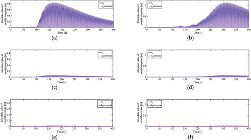Figure 15 shows the absolute value of the actual response and the estimated amplitude. As z(t) is a vertical vibration, it takes only positive values. Thus, the modal responses are compared in terms of absolute values. Regarding vibration control, when tension is used as a control force (for example, (Benosman 2014)), it does not matter whether the horizontal response is positive or not. However, when applying a control force in the horizontal direction, it is necessary to identify the vibration direction using other horizontal sensors. The modal responses are roughly the same in the 1st, 2nd, and 3rd modes, as shown in Figure 15. However, some errors appear between the actual and predicted responses. These are because f_i is an approximate value calculated from the average tension, Z(2f_i) is substituted by the nearest-neighbor value, and the influence of the 4th and 5th modes is also included.

Figure 12. Vertical displacement of the compensating sheave. (a) Heisei 16 Niigata Prefecture Chuetsu Earthquake; (b) 2011 Tohoku Earthquake off the Pacific coast.

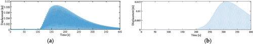
Figure 13. Modal displacements. Five modes are used for numerical analysis, but the responses after the third order are very small. (a) Heisei 16 Niigata Prefecture Chuetsu Earthquake; (b) 2011 Tohoku Earthquake off the Pacific coast.

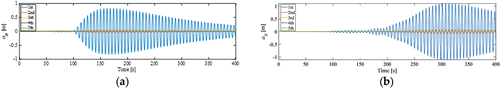
Figure 14. Coefficient of Equation (17)(17) $z_N(t)=\frac{Z(2f_N)}{\sum _{i=1}^{N_0}Z(2f_i)}z(t)\left(N=1,2,\dots ,N_0\right)$(17) (N₀ = 3). The sum of the three values is 1. (a) Heisei 16 Niigata Prefecture Chuetsu Earthquake; (b) 2011 Tohoku Earthquake off the Pacific coast.

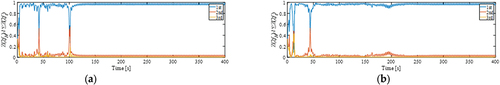
Figure 15. Actual and estimated values of modal responses a_N. (a) 1st mode, (c) 2nd mode, and (e) 3rd mode of the Heisei 16 Niigata Prefecture Chuetsu Earthquake; (b) 1st mode, (d) 2nd mode, and (f) 3rd mode of the 2011 Tohoku Earthquake off the Pacific coast.

4. Conclusion

This paper has described an estimation method in which the vertical vibration of a compensating sheave is distributed to the mode responses based on the predominant frequency of the vertical vibration. The mode-decomposed vertical vibration is then converted into a horizontal mode response using an arc length relational expression.

By applying an FFT with a Hamming window size based on the 1st natural frequency of the rope, it was possible to capture temporal changes in the dominant frequency. Although the proposed method has only been verified with a simplified elevator system, the results demonstrate that one displacement sensor can estimate three vibration modes of the rope.

In future research, we plan to verify the estimation accuracy when the rope does not vibrate in sine wave shapes.

Author contributions

Conceptualization, N.M.; methodology, N.M., T.M., Y.H., H.O. and X.T.N.; software, T.M., N.M. and X.T.N.; validation, N.M., T.M., Y.H., H.O. and X.T.N.; formal analysis, T.M. and N.M.; investigation, X.T.N., N.M. and T.M.; resources, N.M., Y.H. and H.O.; data curation, N.M., T.M., Y.H., H.O. and X.T.N.; writing—original draft preparation, N.M.; writing—review and editing, N.M., T.M., Y.H., H.O. and X.T.N.; visualization, N.M. and T.M.; supervision, N.M.; project administration, N.M.; funding acquisition, N.M. All authors have read and agreed to the published version of the manuscript.

Acknowledgments

This work was supported by JSPS KAKENHI, grant number 21K14389. We thank Stuart Jenkinson, PhD, from Edanz (https://jp.edanz.com/ac) for editing a draft of this manuscript.

Disclosure statement

No potential conflict of interest was reported by the author(s).

Additional information

Notes on contributors

Nanako Miura

Nanako Miura is an Associate Professor of Faculty of Mechanical Engineering, Kyoto Institute of Technology, Kyoto, Japan. She received her Ph.D in Engineering from Keio University. Her research interests include vibration control, structural health monitoring and earthquake disaster countermeasures.

Tomohiro Matsuda

Tomohiro Matsuda is a graduate student of Faculty of Mechanical Engineering, Kyoto Institute of Technology, Kyoto, Japan. He received his BEng from Kyoto Institute of Technology. His research interests include vibration control, elevator,seismic vibration.

Yoshiyuki Higashi

Yoshiyuki Higashi is an Assistant Professor of Faculty of Mechanical Engineering, Kyoto Institute of Technology, Kyoto, Japan. He received his Ph.D in Engineering from the University of Electro-Communications. His research interests include inspection robots, control of drones, indoor navigation, and object detection.

Hiroyuki Ono

Hiroyuki Ono is a Research Associate of Faculty of Mechanical Engineering, Kyoto Institute of Technology, Kyoto, Japan. He received his Ph.D in Engineering from Kyoto Institute of Technology. His research interests include micromechanics, elasticity and plasticity for composite materials.

Xuan Thuan Nguyen

Xuan-Thuan Nguyen is a lecturer at School of Mechanical Engineering, Hanoi University of Science and Technology Hanoi, Vietnam. He received his Ph.D in Engineering from Kyoto Institute of Technology. His research interests include Robotics, Robot control, Structural vibration, vibration control, Optimization.

References

- Benosman, M. 2014. “Lyapunov-based Control of the Sway Dynamics for Elevator Ropes.” IEEE Transactions on Control Systems Technology 22 (5): 1855–1863. doi:10.1109/TCST.2013.2294094.
- Hirose, I., H. Kimura, and K. Ogawa. 2015. “Suppression of Transverse Vibration of Elevator Rope Using Vertical Vibration of Counterweight.” Transactions of the JSME 81. (in Japanese). doi:10.1299/transjsme.15-00102.
- Hucheng, W., D. Zhang, and Q. Cheng. 2019. “Modeling and Parameters Analysis of Longitudinal Vibration of high-velocity Elevator Hoisting System.” ICIC Express Letters, Part B: Applications 10: 97–103. doi:10.24507/icicelb.10.02.97.
- Ito, H., M. Morishita, and H. Kimura. 2006. “The Modeling of Longitudinal and Lateral Vibrations on the Elevator Rope.” Transactions of the Japan Society of Mechanical Engineers Series C 72 (717): 1435–1439. (in Japanese). doi:10.1299/kikaic.72.1435.
- Kaczmarczyk, S., R. Iwankiewicz, and Y. Terumichi. 2009. “The Dynamic Behaviour of a non-stationary Elevator Compensating Rope System under Harmonic and Stochastic Excitations.” Journal of Physics: Conference Series 181: 1–8. doi:10.1088/1742-6596/181/1/012047.
- Kimura, H. 2016. “Free Vibration Analysis of a String with Vibration Suppressor (When the Position of Vibration Suppressor Is Opposite to the Pulled Position).” Mechanical Engineering Journal 3 (1): 15–00554-15–00554. doi:10.1299/mej.15-00554.
- Kimura, H., and T. Kuguminato. 2013. “Simplified Calculation Method for Detecting Elevator Rope Deflection during Earthquake (Considering the Distribution of Rope Tension).” Journal of System Design and Dynamics 7: 343–354. doi:10.1299/jsdd.7.343.
- Kubo, T., Y. Hisada, S. Horiuchi, and S. Yamamoto. 2009. “Application of long-period Ground Motion Prediction Using Earthquake Early Warning System to Elevator Emergency Operation Control System of a high-rise Building.” Journal of Japan Association for Earthquake Engineering 9: 31–50. (in Japanese). doi:10.5610/jaee.9.2_31.
- Miura, N., and M. Kohiyama. 2012. “Vibration Suppression of a building-elevator System Adjusted to Ground Motion Intensity and Level of Building Responses Using a Control Device of the Building.” In Proceedings of the 15th World Conference on Earthquake Engineering, Portugal; Vol. 278, 1–10.
- Miura, N., and A. Sone. 2019. “Relation between the Tension Load and Rope Sway of an Elevator Operating in a Building under Sinusoidal Excitation: Active Vibration Control for the Operation of an Elevator during an Earthquake: Part 1.” Journal of Structural and Construction Engineering (Transactions of AIJ) 84: 917–926. (in Japanese). doi:10.3130/aijs.84.917.
- National Research Institute for Earth Science and Disaster Resilience, NIED K-NET, KiK-net, National Research Institute for Earth Science and Disaster Resilience. 2019. doi:10.17598/NIED.0004.
- Nguyen, X. T., N. Miura, and A. Sone. 2019. “Optimal Design of Control Device to Reduce Elevator Ropes Responses against Earthquake Excitation Using Genetic Algorithms.” Journal of Advanced Mechanical Design, Systems, and Manufacturing 13 (2): 1–18. doi:10.1299/jamdsm.2019jamdsm0038.
- Oppenheim, A. V., R. W. Schafer, and J. R. Buck. 1999. Discrete-time Signal Processing, 468–471. New Jersey, USA: Prentice Hall.
- Otsuki, M., Y. Ushijima, K. Yoshida, H. Kimura, and T. Nakagawa. 2006. “Application of Nonstationary Sliding Mode Control to Suppression of Transverse Vibration of Elevator Rope Using Input Device with Gaps.” JSME International Journal, Series C: Mechanical Systems, Machine Elements and Manufacturing 49: 385–394. doi:10.1299/jsmec.49.385.
- Peng, Q., A. Jiang, H. Yuan, G. Huang, H. Shan, and L. Shanqing. 2020. “Study on Theoretical Model and Test Method of Vertical Vibration of Elevator Traction System.” Mathematical Problems in Engineering 1–12. doi:10.1155/2020/8518024.
- Shuiyuan, W., H. Ping, and X. Gong. 2021. “Analysis of Transverse Vibration of Wire Rope in Flexible Hoisting System.” Journal of Vibroengineering 23 (2): 283–297. doi:10.21595/jve.2020.21487.
- Takumi, R., and H. Utsuno. 2022. “Damping Force of Air Acting on Vibrating Elevator Rope.” Mechanical Engineering Journal 9 (1): 1–13. doi:10.1299/mej.21-00320.
- Teshima, N., Y. Sasaki, S. Onishi, and M. Nagai. 2002. “Vibration Characteristics of wire-rope in the High Speed Elevator (Numerical Analysis by the Difference Method).” Transactions of the Japan Society of Mechanical Engineers Series C 68 (675): 3202–3208. (in Japanese). doi:10.1299/kikaic.68.3202.
- Watanabe, S. 2020. “Coupled Vibration Mechanism between Vertical and Horizontal Direction against Elevator Rope.” In Proceedings of the Elevator, Escalator and Amusement Rides Conference, Japan, Vol. Paper no. 108. (in Japanese). doi:10.1299/jsmeearc.2020.108
- Watanabe, S., and T. Okawa. 2018. “Vertical Vibration of Elevator Compensating Sheave Due to Brake Activation of Traction Machine.” Journal of Physics: Conference Series 1048: 1–7. doi:10.1088/1742-6596/1048/1/012012.
- Watanabe, S., T. Okawa, D. Nakazawa, and D. Fukui. 2013. “Vertical Vibration Analysis for Elevator Compensating Sheave.” Journal of Physics: Conference Series 448: 012007. doi:10.1088/1742-6596/448/1/012007.
- Xiujuan, Q., R. Zhanga, and H. Qin. 2019. “Modeling and Analysis of Transverse Vibration of Traction Rope of High Speed Traction Elevator.” Materials Science and Engineering 538: 1–7. doi:10.1088/1757-899X/538/1/012036.
- Yang, D.-H., K.-Y. Kim, M. K. Kwak, and S. Lee. 2017. “Dynamic Modeling and Experiments on the Coupled Vibrations of Building and Elevator Ropes.” Journal of Sound and Vibration 390: 164–191. doi:10.1016/j.jsv.2016.10.045.
- Zhang, Q., Y.-H. Yang, T. Hou, and R.-J. Zhang. 2019. “Dynamic Analysis of high-speed Traction Elevator and Traction car–rope time-varying System.” Noise & Vibration Worldwide 1–9. doi:10.1177/0957456519827929.