Reverse design charts for flexural strength of steel-reinforced concrete beams based on artificial neural networks

ABSTRACT

Design of steel-reinforced concrete (SRC) beams can be a lengthy process, and understanding how design parameters as many as over 26 influence each other can be difficult. In this study, an artificial neural network was trained with large structural datasets to realize a reverse design of SRC beams based on mapping input parameters to output parameters rather than on structural mechanics or knowledge. For training, a back-substitution method was applied in two steps: reverse outputs are calculated in a reverse network of Step 1 for given reverse input parameters; then, reverse output parameters obtained in Step 1 are substituted as input parameters in forward network of Step 2 to obtain design parameters. Trained network was then implemented in determining design parameters of SRC beams for given unseen structural input parameters. Network results were ascertained through conventional structural calculations. Design charts offer predictions of multiple design parameters in any order, which can help engineers in the preliminary design of SRC beams. The developed network can be used to explore intricacies of design parameters to each other, which may be difficult with conventional design methods.

GRAPHICAL ABSTRACT

KEYWORDS:

• Artificial neural network
• reverse design
• network training
• AI-based design chart
• SRC beam design based on AI

1. Introduction

Several studies have focused on using neural networks for analysis and design. Vanluchene and Sun (1990) used neural networks to identify the location and magnitude of the maximum bending moment of a simply supported rectangular plate. Hajela and Berke (1991) used neural networks for design optimization, where the input data comprised the length and height of a truss, while the output data comprised the optimized bar area and total weight of the truss. Flood and Kartam (1994a, 1994b) and Hong (2019) conceptualized the application of neural networks to structural engineering by exploring the influence of the number of hidden layers and hidden nodes on network validation and processing speed. Wu and Jahanshahi (2019) proposed applying convolutional neural network (CNN) to noisy data to predict the structural response more accurately than the multilayer perceptron (MLP) algorithm. They presented a deep CNN-based approach to estimating the dynamic response of a linear single-degree-of-freedom (SDOF) system, nonlinear SDOF system, and full-scale three-story multi-degree-of-freedom steel frame. Lavaei and Lohrasbi (2012) presented a backpropagation wavelet neural network based on the scaled conjugate gradient algorithm, where they replaced the sigmoid activation functions of hidden layer neurons with wavelets to approximate the dynamic time history response of frame structures. Fahmy, El-Madawy, and Gobran (2016) developed a methodology for using an artificial neural network (ANN) in the conceptual design of orthotropic steel deck bridges. They found that ANNs prove to be a better, more cost-effective design option than international codes or expert opinion. Adeli has published numerous articles on structural analysis and design problems since 1989 (Adeli 2001). Lee et al. (2018) noted that neural networks have demonstrated limitations and numerical instability in structural engineering because of their poor performance and very high computation time, especially for complicated problems with multiple hidden layers. Gupta and Sharma (2011) also found that neural network applications in structural engineering have greatly decreased over the last decade. Application of ANNs has been performed successfully in many studies of researchers since the early 1900s for predicting capacity of pile foundations under axial and lateral loads Chan, Chow, and Liu 1995, Lee and Lee 1996, Rahman et al. 2001, Hanna, Morcous, and Helmy 2004, Das and Basudhar 2006), designing and optimizing weights of steel and truss structures (Adeli and Park 1995a, 1995b, Tashakori and Adeli 2002, Kang and Yoon 1994), calculating tunnels and underground opening structures (Lee and Sterling 1992, Shi, Ortigao, and Bai 1998, Shi 2003, Neaupane and Achet 2004, Yoo and Kim 2007), and predicting seismic responses of building structures and bridges (Oh et al. 2020, Lagaros and Papadrakakis 2012, Asteris et al. 2019, 2009,Huang and Huang 2020). Recently, the available computational power for routine training has been greatly enhanced using multiple graphics processing units (GPUs), which has let researchers train larger networks to overcome the above limitations and numerical instability.

Many studies have concluded that a successful neural network implementation depends on the quality of the training data. However, many such studies only focused on verifying the training accuracy rather than application of networks to the practical design of structures with unseen input parameters by networks. Little literature is available on applying ANNs to structural design in general and to steel-reinforced concrete (SRC) beams in particular. Notably, ANNs were successfully used to implement in designing beams and columns in the studies of Hong, Pham, and Nguyen (2021), Hong, Nguyen, and Nguyen (2021), Hong and Nguyen (2021), and Hong and Pham (2021). Specifically, the optimization issues can be solved by neural networks with acceptable accuracies for helping engineers in designing concrete members to control any design parameters and to reduce costs and CO₂ emission in construction. In the present study, neural networks are suggested to provide practical design solutions for SRC beams. In the proposed network, the positions of the network inputs and outputs are exchanged for a reverse design. This is especially useful when multiple design parameters are reversed, which is not possible with conventional design methods where output parameters are obtained for given input parameters. This study suggests an AI-based reverse design method which presents applicable design charts when calculation sequences of inputs and outputs are exchanged. The network accuracy for the SRC design was verified through conventional structural calculations. The innovative design charts offer practical application to SRC beams. The fast and accurate determination of design parameters for both forward and reverse designs of SRC beams become available, enabling engineers to use them to obtain preliminary design parameters for SRC beams and to predict multiple design parameters in any order. Robust design of SRC beams based on design charts is also possible, which is challenging to achieve with conventional design methods. As a demonstration, the proposed network was applied to designing SRC beams encasing an H-shaped steel section with 15 input parameters and 11 output parameters.

2. Artificial intelligence-based design scenarios for SRC beams

Figure 1 shows the dimensions of an SRC beam, including the beam height (h) and width (b). The beam section comprises rebar and steel sections encased by concrete. Table 1 presents the scenarios for an SRC beam encasing an H-shaped steel section: four reverse designs (Reverse Scenarios 1–4). In the conventional calculation referred to a forward design, 11 output parameters (Engineering outputs shown in Table 1) were calculated based on 15 input parameters (Engineering inputs shown in Table 1). However, safety factor (SF) and tensile rebar strain (ε_rt) cannot be predicted in forward design, and hence, Reverse Scenarios 1–4 were established to pre-assign a safety factor (SF) and a tensile rebar strain (ε_rt) that were output parameters of forward design as input parameters to control a design moment, which is a significant challenge to the conventional method. Two input parameters in forward design were set as output parameters in Reverse Scenarios 1–4 (b and b_s for Reverse Scenarios 1; ρ_rc and t_f for Reverse Scenarios 2; ρ_rt and ρ_rc for Reverse Scenarios 3; d and ρ_rt for Reverse Scenarios 4) as indicated in Table 1. Beam length (L), material properties (concrete strength (f’_c), rebar strength (f_y), steel strength (f_yS)), and imposed loads (moment due to dead load (M_D) and moment due to live load (M_L)) are pre-assigned on an input side.

Figure 1. Geometry of SRC beam.

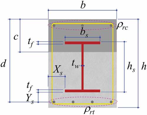
Table 1. Scenario table for SRC beam.

3. Generation of large datasets

3.1. Material and manufacturing prices for calculating the cost index (CI_b) of SRC beams

Hong et al. (2010) calculated the CO₂ emissions of concrete and metals during construction. They found that one ton of metal emits 2.513 t-CO₂ during construction stage, while 1 m³ of concrete emits 0.1677 t-CO₂. These data may vary slightly from those of other studies. Cost index (CI_b) included material and manufacturing prices of all components for an SRC beam per 1 m length. Tables 2–4 present the unit prices for the various materials comprising the SRC. These unit prices may vary due to market volatility, but they were assumed to remain constant during this study. The concrete unit price clearly depended on the concrete strength as presented in Table 2. The rebar unit price did not depend greatly on the rebar strength and varied from 1055 to 1085 Korean won (KRW)/kgf for rebar strengths of 500–600 MPa, respectively. The steel unit price slightly varied from 1800 to 1880 KRW/kgf related to steel strengths of 275–325 MPa. The data are subject to change.

Table 2. Concrete unit price versus concrete strength.

Concrete strength (MPa)	Concrete unit price (KRW/m^3)
30	85,000
40	94,000
50	104,000

Table 3. Rebar unit price versus rebar strength.

Rebar strength (MPa)	Rebar unit price (KRW/kgf)
500	1055
600	1085

Table 4. Steel unit price versus steel strength.

Steel strength (MPa)	Steel unit price (KRW/kgf)
275	1800
325	1880

3.2. Generation of large datasets

The artificial neural networks (ANNs) are formulated to have an ability to generalize trends (recognized as the machine learning) between inputs and outputs for the engineering designs rather than being based on the engineering mechanics or knowledge (Hong 2019; Berrais 1999). AI-based designs do not depend on the structural mechanics and theory but on big datasets which are generated by any given structural software, while some softwares are simple and some are very complex. Big datasets are complex if the structural calculations are complex, then, engineers may have to select an appropriate training method (Hong, Pham, and Nguyen 2021) with a number of layers, neurons, epochs, validations etc. to properly train ANNs on complex big data. It is noted that an adequacy of an ANN depends on good training datasets. The data generation and training algorithms are programmed based on MATLAB Deep Learning Toolbox (MathWorks 2022), MATLAB Parallel Computing Toolbox (MathWorks 2022), MATLAB Statistics and Machine Learning Toolbox (MathWorks 2022), and MATLAB R2022a (MathWorks 2022).

In this study, the ANNs are trained on the big datasets generated by the SRC software the authors developed for a shallow SRC beam design which is verified and published in Nguyen and Hong (2019). The flowchart to calculate flexural behavior of shallow SRC beams neglecting shear deformations is demonstrated in Figure 2(a). The authors would like to add an interaction of flexural behaviors of SRC beams with shear behaviors in the future research. The authors will continue to revise this software constantly to better predict the behavior of SRC beams, which then will be used to update big datasets. However, the authors would like this study to show that ANNs proposed in this study can be re-trained with updated number of layers, neurons, epochs, validations checks even when big datasets are updated by the updated software. This is one of the significant contributions of this study, proposing how to derive generalizable AI-based networks with big datasets that may be updated based on future SRC software. AI-based networks only see the big datasets generated by the given software, not being able to correct and revise the big data, and hence, revising big datasets belongs to engineers.

Figure 2. Structural mechanics-based software for SRC beam.

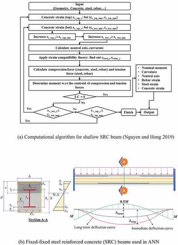
Figure 2(b) shows the SRC beam section with fixed ends that was used for the artificial intelligence (AI)-based design. The dimensions of the beam were the width (b) × effective depth (d) × length (L). The beam was subjected to a uniform load, which resulted in an immediate deflection (∆_imme) and long-term deflection (∆_long). According to the American Concrete Institute (ACI) design code, the immediate deflection (∆_imme) due to a live load should be less than L/360, and the long-term deflection (∆_long) due to sustained loads with additional live load should be less than L/240. Large datasets were generated based on the algorithm shown in Figure 3. SRC beams were designed by structural mechanics using a strain compatibility-based theory (called AutoSRCbeam), which was developed by Nguyen and Hong (2019). AutoSRCbeam was used to generated large datasets. Input parameters were established randomly, from which output parameters were also obtained randomly. The beam length (L) and effective depth (d) were randomly selected within 6000–12,000 mm and 400–1445 mm, respectively, while the beam width (b) was randomly selected within 0.3–0.8 h. Table 5 presents the nomenclature and ranges of random values for the input parameters of the SRC beam. In this flowchart, all 15 input parameters for forward design were randomly selected in pre-assigned ranges; thus, 11 output parameters were calculated based on AutoSRCbeam. Tensile rebar ratios (ρ_rt) were randomly generated in the range [ρ_rt,min; ρ_rt,max], therein, ρ_min was set by formula of ACI code (${\rho }_{rt}{,}_{min}=max\left[1.4/f_y;\sqrt{f_c^{\prime }}/4f_y\right]$); ρ_rt,max was set at a value of 0.05. Compressive rebar ratios (ρ_rc) were randomly generated in range [${\rho }_{rt}/400;0.5{\rho }_{rt}$]. Tensile rebar strains are, then, calculated based on AutoSRCbeam. According to the ACI code 318–19, the tensile rebar strain (ε_rt) should be no less than 0.003 + ε_y (ε_y is yield strain of rebar). In case the tensile rebar strain (ε_rt) was smaller than 0.003 + ε_y, tensile rebar ratios (ρ_rt) and compressive rebar ratios (ρ_rc) were randomly generated again to calculate new tensile rebar strains (ε_rt) to be greater than 0.003 + ε_y. This process was repeated until ACI 318–19 condition was satisfied (ε_rt ≥ ε_y + 0.003). Finally, 100,000 datasets were generated, each dataset consisted of a total of 26 parameters (15 inputs and 11 outputs), then, these big structural datasets were used to train neural networks as demonstrated in Figure 3. The gross beam height was eliminated as a parameter because h was not trained as a random variable. The concrete clear cover was not random but fixed at 40 mm. The ACI code defines the combined load M_{u (including Ms)} = 1.2M_D + 1.6M_L + 1.2 M_s. The design moment strength is given by

Figure 3. Flowchart for large structural datasets of SRC beams used to train network (Nguyen and Hong 2019, Nguyen 2021).

(1) $\varphi {M_n}_{(includingMs)}\ge {M_u}_{(includingMs)}=\hspace{0.17em}1.2M_D+\hspace{0.17em}1.6M_L+\hspace{0.17em}1.2M_s$(1)

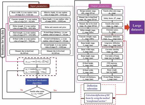
Table 5. Nomenclatures and ranges of parameters defining SRC beams (Nguyen 2021) .

Notation			Range
Input parameters	L (mm)	Beam length	[6000$\sim$12,000]
	d (mm)	Effective beam depth	[400$\sim$1445]
	b (mm)	Beam width	[150$\sim$1200]
	fc’(MPa)	Concrete strength	[30$\sim$50]
	fy (MPa)	Rebar strength	[500$\sim$600]
	ρrt	Tensile rebar ratios	${\rho }_{rt,min}=max\left(\frac{0.25\sqrt{f_c^{\prime }}}{f_y};\frac{1.4}{f_y}\right)$
	ρrc	Compressive rebar ratios	[1/400$\sim$1/2] ρrt
	hs (mm)	H-shaped steel height	[5~1180]
	bs (mm)	H-shaped steel width	[45$\sim$700]
	tf (mm)	H-shaped steel flange thickness	[5$\sim$30]
	tw(mm)	H-shaped steel web thickness	[5$\sim$30]
	fyS (MPa)	Steel strength	[275$\sim$325]
	Ys (mm)	Clearance between H steel section and closest rebar layer	[60~963]
	MD (kN·m)	Moment due to dead load	$\left[0.2\sim \frac{1}{1.2}\right]M_u$
	ML (kN·m)	Moment due to service live load	$\frac{1}{1.6}\left(M_u-1.2M_D\right)$
	SF	Safety factor SF = $\varphi$Mn/Mu Where, $\varphi$Mn: Design moment excluding self-weight Mu: Factored moment, Mu = 1.2MD + 1.6ML	[1~2]
Output parameters	$\varphi$Mn (kN·m)	Design moment without considering effect of self-weight at εc = 0.003
	εrt	Tensile rebar strain at εc = 0.003	εrt ≥ εy + 0.003
	εst	Strain of tensile steel flange at εc = 0.003
	Δimme.(mm)	Immediate deflection due to ML service live load	(Δimme. ≤ L/360, ACI 318–19)
	Δlong (mm)	Sum of long-term deflection due to sustained loads and immediate deflection due to additional live load	(Δlong ≤ L/240, ACI 318–19)
	μ$\varphi$	Curvature ductility, μ$\varphi$ = $\varphi$μ/$\varphi$y, Where, $\varphi$μ: Curvature at εc = 0.003 $\varphi$y: Curvature at tensile rebar yield
	CIb (KRW/m)	Cost index per 1 m length of beam
	CO2 (t-CO2/m)	CO2 emission per 1 m length of beam
	BW (kN/m)	Beam weight per 1 m length of beam
	XS (mm)	Clearance between flange of H steel section and edge of beam Xs = 0.5(b – bs)

where M_D,M_L, and M_s are moments due to the dead load, live load, and self-weight, respectively. However, the design load does not include the self-weight of the structure:

(2) $\varphi M_n=\varphi {M_n}_{(includingMs)}-1.2M_s\ge M_u=1.2M_D+1.6M_L$(2)

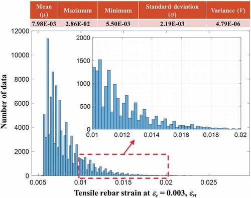
M_s due to the self-weight was not considered as a parameter during training to avoid input conflict because the dimensions of the beam section are not known during the training and design stages. Input conflicts may be caused if all of M_D,M_L,M_s, and $\varphi$M_n are used as dimensions without the beam sections being known. Table 6 presents the mean, standard deviation, and variance of randomly selected design inputs and outputs based on 100,000 datasets generated for SRC beams. Figure 4(1)–(23) shows the distributions of all input and output parameters. The beam length (L), beam depth (d), flange thickness of the steel section (t_f), web thickness of the steel section (t_w), concrete strength (f’_c), rebar strength (f_y), and steel strength (f_yS) were randomly selected with uniform distributions within minimum and maximum values, whereas others were found to distribute with a bell-shaped distribution. Figure 4(13)–(16) presents the histograms of the moment due to the dead load (M_D), moment due to the live load (M_L), design moment ($\varphi$M_n), and tensile rebar strain at ε_c = 0.003 (ε_rt). These parameters were generated based on severe nonlinearities, which led to skewed data distributions. Therein, the range of beam length (L) was from 6000 mm to 12,000 mm, whereas the distribution of beam length (L) data was uniform as shown in Figure 4(1), resulting in the mean of beam length (L) data of 8994.3 mm, which is close to an average of minimum and maximum of the data range (9000 mm); the standard deviation and variance were found as 1744.6 mm and 3,043,577.9 mm², respectively. Means, standard deviations, variances, and histograms of all parameters (inputs and outputs) for SRC beams can be found in Table 6 and Figure 4(1)–(23).

Figure 4. Distribution of ranges of input and output parameters with 100,000 datasets.

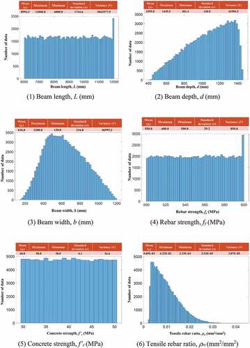
Figure 4. (Continued).

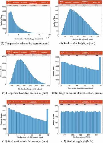
Figure 4. (Continued).

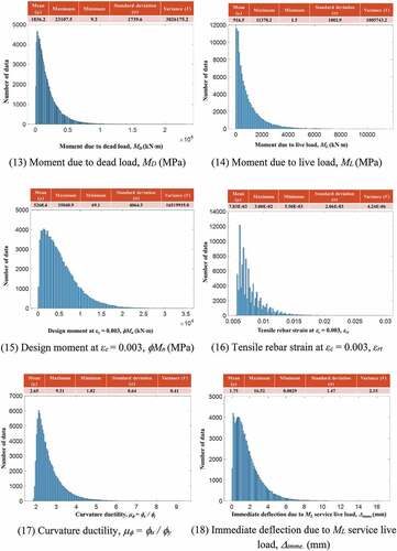
Figure 4. (Continued).

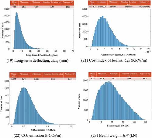
Table 6. Means, standard deviations, and variances of random design inputs and outputs for SRC beams.

	Parameter	Mean (μ)	Maximum	Minimum	Standard deviation (σ)	Variance (V)
Inputs	L (mm)	8994.3	12,000.0	6000.0	1744.6	3,043,577.9
	d (mm)	1059.8	1445.5	401.4	248.8	61,904.5
	b (mm)	636.0	1200.0	150.0	216.8	46,995.2
	fy (MPa)	550.0	600.0	500.0	29.2	850.0
	fc’ (MPa)	40.0	50.0	30.0	6.1	36.6
	ρrt	9.89E-03	4.32E-02	2.33E-03	5.54E-03	3.07E-05
	ρrc	2.97E-03	1.94E-02	6.50E-06	2.55E-03	6.51E-06
	hs (mm)	496.1	1180.0	5.0	238.3	56,797.9
	bs (mm)	280.0	700.0	45.0	114.1	13,012.2
	tf (mm)	16.3	30.0	5.0	7.5	55.9
	tw (mm)	15.8	30.0	5.0	7.4	54.4
	fyS (MPa)	300.0	325.0	275.0	14.7	216.1
	Ys (mm)	293.7	962.6	60.0	159.8	25,524.6
	MD (kN·m)	1836.2	23,107.5	9.3	1739.6	3,026,175.2
	ML (kN·m)	916.5	11,370.2	1.5	1002.9	1,005,743.2
Outputs	$\varphi$Mn (kN·m)	5268.4	35,040.9	69.1	4064.5	16,519,919.0
	εrt	7.83E-03	3.00E-02	5.50E-03	2.06E-03	4.24E-06
	εst	4.50E-03	2.51E-02	−3.00E-04	2.19E-03	4.80E-06
	Δimme. (mm)	1.75	16.52	0.0029	1.47	2.15
	Δlong (mm)	7.93	67.06	0.43	5.35	28.66
	μ$\varphi$	2.65	9.31	1.82	0.64	0.41
	CIb (KRW/m)	407,748.4	1,579,803.8	30,450.4	202,079.7	40,836,203,417.2
	CO2 (t-CO2/m)	0.683	3.063	0.051	0.351	0.123
	BW (kN/m)	20.25	52.36	2.03	9.80	96.11
	XS (mm)	178.0	420.0	30.0	66.4	4415.5
	SF	1.50	2.00	1.00	0.30	0.09

4. Networks based on back-substitution

Structural steel in SRC beams contributes its strength and rigidity to a flexural and shear behavior simultaneously, making a design procedure complex. However, training for ANNs to design such SRC beams are not difficult as long as SRC beams are regular in shapes. The authors showed AI-based designs for RC beams (Hong, Pham, and Nguyen 2021; Hong, Nguyen, and Nguyen 2021; Hong and Pham 2021; Nguyen 2021; Hong, Nguyen, and Nguyen 2021; Pham and Hong 2022), RC columns (Hong and Nguyen 2021; Hong, Nguyen, and Pham 2022; Hong et al. 2022), and SRC columns (Hong et al. 2022a, 2022b) in their previous papers. AI-wise, the complexities related to structural configurations may cause some difficulties in training due to complicated relationships among parameters defining configurations of the structures under consideration. In the previous studies of the authors, useful training methods, including TED, PTM, or CRS, (Hong, Pham, and Nguyen 2021), were developed based on appropriate training parameters including a number of layers, neurons, the maximum epoch, and validation, etc., to perform trainings of diverse structural systems.

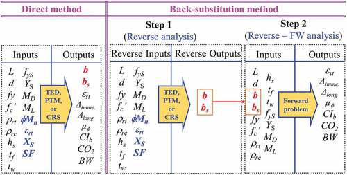
The direct and back-substitution (BS) methods were implemented in this study, as shown in Figure 5. The direct method required only one step for training and design. In contrast, the BS method required two steps for training: input parameters for the forward network of Step 2 were calculated as the reverse outputs in the network of Step 1 for given reverse input parameters; and the reverse output parameters in Step 1 were then substituted as input parameters in Step 2 to obtain the design parameters. The training on entire data, parallel training method (PTM), and chained revised sequence (CRS) (Hong, Pham, and Nguyen 2021, Hong, Nguyen, and Nguyen 2021, Hong 2021) algorithms can be used in both the direct and the reverse network of Step 1 of BS methods. By direct method (Hong, Pham, and Nguyen 2021) shown in Figure 5, nine output parameters (b, b_s,ε_st,∆_imme,∆_long,µ_$\varphi$,CI_b, CO₂, and BW) were calculated directly from 17 input parameters (L, d, f_y,f’_c,ρ_rt,ρ_rc,h_s,t_f,t_w,f_yS,Y_s,M_D,M_L,$\varphi$M_n,ε_rt, SF, and X_s), among which design moment ($\varphi$M_n), tensile rebar strain (ε_rt), clearance (X_s), and safety factor (SF) are the reverse inputs of neural networks. Direct method needs only one step to finish mapping. However, the BS method needs two steps (Hong, Nguyen, and Nguyen 2021). In the first step, 17 input parameters which are identical used in direct method are mapped to only two reverse output parameters (b, and b_s). In the second step, a forward calculation using structural software is followed as indicated in Figure 5. Step 2 of the BS method can be performed by any engineering software with 15 input parameters (L, d, b, b_s,f_y,f’_c,ρ_rt,ρ_rc,h_s,t_f,t_w,f_yS,Y_s,M_D,M_L) for SRC beams. It is clear to see that a BS method gives more accurate results than the direct method because it omits reverse output parameters (b, and b_s) from output parameters when training networks.

Figure 5. Direct and back-substitution methods.

5. Reverse Scenarios

5.1. Reverse Scenario 1

In Reverse Scenario 1 (see Table 1), nine output parameters (b, b_s,ε_st,∆_imme,∆_long,µ_$\varphi$,CI_b, CO₂, and BW) were determined from 17 input parameters ($\varphi$M_n,ε_rt, SF, X_s, L, d, f_y,f’_c,ρ_rt,ρ_rc,h_s,t_f,t_w,f_yS,Y_s,M_D, and M_L). Among the input parameters, the reverse inputs were the design moment ($\varphi$M_n), tensile rebar strain (ε_rt), safety factor (SF), and longitudinal clearance between the beam edge and H-shaped steel section (X_s) (green numbers in Table 7(a–c)). The widths of the concrete and steel sections (b and b_s) were obtained on the output side (purple numbers) as reverse output parameters. The material properties of the concrete, rebar, and steel (f’_c,f_y, and f_yS); concrete geometry (L and d); steel dimensions (h_s,t_f, and t_w); rebar ratios (ρ_rt and ρ_rc); design moment ($\varphi$M_n); and lower clearance between a rebar layer and H-shaped steel section (Y_s) were assigned to the input side when they are predetermined by engineers. In the first step of the BS method, a shallow neural network (SNN) was used to map the 17 input parameters (red and green numbers) ($\varphi$M_n,ε_rt, SF, X_s, L, d, f_y,f′_c,ρ_rt,ρ_rc,h_s,t_f,t_w,f_yS,Y_s,M_D,M_L) to the two reverse output parameters (purple numbers) (b and b_s) with the PTM. First training network includes 17 input parameters (red and green numbers) and one output parameter (b) where four hidden layers and 50 neurons were implemented with 49,991 epochs, resulting in mean squared error (MSE) = 7.94 × 10⁻⁴ and Regression (R) index = 1.0. Second network determined width of H-shaped steel section (b_s) on output side by mapping 17 inputs (red and green numbers) where five hidden layers and 50 neurons were performed with 49,995 epochs, resulting in MSE = 1.71 × 10⁻⁵ and Regression (R) index = 0.9999.

Table 7. Design table for Reverse Scenario 1 with 17 input parameters and nine output parameters based on reverse PTM- forward AutoSRCbeam with $\varphi$M_n = 2,000 kN⋅m, $\varphi$M_n = 3,000 kNm, $\varphi$M_n = 4,000 kN⋅m, and ε_rt = 0.008.

In the second step of the forward network, the input and output relationships were established according to structural mechanics (AutoSRCbeam software). Seven forward output parameters (ε_st,∆_imme,∆_long,µ_$\varphi$,CI_b, CO₂, BW) (dark red numbers) were calculated by using 15 input parameters (L, b, d, f_y,f’_c,ρ_rt,ρ_rc,h_s,b_s,t_f,t_w,f_yS,Y_s,M_D, and M_L) (pink numbers) that were identical to 13 ordinary inputs (red numbers) and two reverse output parameters (b and b_s) (purple numbers) from Step 1. Design moment ($\varphi$M_n), tensile rebar strain (ε_rt), safety factor (SF), and X_s (green numbers) were not calculated in the second step because they were preassigned as reverse input parameters. To verify the BS network results, 15 parameters (L, d, b, f_y,f’_c,ρ_rt,ρ_rc,h_s,b_s,t_f,t_w,f_yS,Y_s,M_D, and M_L) (blue numbers) were used as input parameters for the AutoSRCbeam software to calculate four forward output parameters ($\varphi$M_n,ε_rt, SF, and X_s) (light blue numbers) for comparison.

Three SRC beams were designed for design moments ($\varphi$M_n) of 2000, 3000, and 4000 kN⋅m and a fixed tensile rebar strain (ε_rt) of 0.008 as presented in Table 7(a–c). Insignificant errors were observed with values of 0.74%, 0.16%, and −0.07% corresponding to the design moments ($\varphi$M_n) as can be seen in Table 7(a–c), respectively. Maximum percentage errors were obtained with values of 2.50%, 5.00%, and 6.25% corresponding to tensile rebar strain (ε_rt) as indicated in Table 7(a–c). Some input parameters were adjusted for the three designs to avoid input conflicts among the reverse input parameters. Three SRC beams shared the same material properties and geometry (L = 10,000 mm, d = 1000 mm, f_y = 500 MPa, f’_c = 30 MPa, ρ_rt = 0.003, ρ_rc = 0.002, h_s = 600 mm, t_f = 15 mm, t_w = 6 mm, f_yS = 325 MPa, Y_s = 230 mm, M_D = 500 kN⋅m, M_L = 500 kN⋅m) except for beam widths (b). In Table 7(a–c), the design moments were 2000 kN∙m, 3000 kN∙m, and 4000 kN∙m, resulting in calculated beam widths of 517.1 mm, 744.1 mm, and 970.7 mm, respectively. The increased beam width resulted in stronger SRC beams, leading to the reduction of deflections (immediate (Δ_imme.) and long-term deflection (Δ_long)). The beam widths were 517.1 mm, 744.1 mm, and 970.7 mm, resulting in 2.40 mm, 1.36 mm, and 0.81 mm for immediate deflections and 6.14 mm, 3.10 mm, and 2.77 mm for long-term deflections, respectively. Observation showed that tensile rebar strains (ε_rt) were almost the same (0.0068, 0.0067, and 0.0066), leading to the same curvature ductility (μ_$\varphi$ = 2.86, 2.79, and 2.77) of three SRC beams as indicated in Table 7(a–c).

5.2. Reverse Scenario 2

In Reverse Scenario 2 (see Tables 1 and 10), output parameters (ρ_rc,t_f,ε_st,∆_imme,∆_long,µ_$\varphi$,CI_b, CO₂, BW, and X_s) were determined from 16 input parameters ($\varphi$M_n,ε_rt, SF, L, d, b, f_y,f′_c,ρ_rt,h_s,b_s,t_w,f_yS,Y_s,M_D, and M_L). Among the input parameters, the reverse inputs were the design moment ($\varphi$M_n), tensile rebar strain (ε_rt), and safety factor (SF) (green numbers in Table 8(a–c)). The compressive rebar ratio and flange thickness of the steel section (ρ_rc and t_f) were obtained on the output side (purple numbers) as reverse output parameters. The material properties of the concrete, rebar, and steel (f′_c,f_y, and f_yS); concrete geometry (L, d, and b); steel dimensions (h_s,b_s, and t_w); rebar ratio (ρ_rt); design moment ($\varphi$M_n); and lower clearance between a rebar layer and H-shaped steel section (Y_s) were also assigned to the input side under the assumption that they were predetermined by engineers. In the first step of the BS method, an SNN was used to map 16 input parameters ($\varphi$M_n,ε_rt, SF, L, d, b, f_y,f′_c,ρ_rt,h_s,b_s,t_w,f_yS,Y_s,M_D,M_L) (red and green numbers) to two reverse output parameters (ρ_rc,t_f) (purple cells) with the PTM. First training network included 16 input parameters (red and green numbers) and one output parameter (ρ_rc) where five hidden layers and 50 neurons were performed with 27,166 epochs, resulting in MSE = 8.14 × 10⁻⁴ and R = 0.9952. Second network calculated flange thickness of H-shaped steel section (t_f) on output side by mapping 16 inputs (red and green numbers) where five hidden layers and 50 neurons were implemented with 16,716 epochs, resulting in MSE = 1.40 × 10⁻² and R = 0.9814.

Table 8. Table design for Reverse Scenario 2 with 16 input parameters and 10 output parameters based on reverse PTM – forward AutoSRCbeam with ε_rt = 0.009, ε_{rt =} 0.012, ε_{rt =} 0.015, and $\varphi$M_n (kN·m) = 3000.

Table 9. Table design for Reverse Scenario 3 with 16 input parameters and 10 output parameters based on reverse PTM- forward AutoSRCbeam with ε_rt = 0.008, ε_rt = 0.010 and ε_rt = 0.012, and $\varphi$M_n (kN·m) = 3500.

Table 10. Table design for Reverse Scenario 4 with 16 input parameters and 10 output parameters based on reverse PTM- forward AutoSRCbeam with ε_rt = 0.008, ε_rt = 0.012 and ε_rt = 0.020, and $\varphi$M_n (kN·m) = 3500.

In the second step of the forward network, the input and output relationships were established according to structural mechanics (AutoSRCbeam software). Eight forward output parameters (ε_st,∆_imme,∆_long,µ_$\varphi$,CI_b, CO₂, BW, X_S) (dark red numbers) were calculated from 15 input parameters (L, b, d, f_y,f′_c,ρ_rt,ρ_rc,h_s,b_s,t_f,t_w,f_yS,Y_s,M_D, and M_L) (pink numbers) that were identical to 13 ordinary inputs (red numbers) and two reverse output parameters (ρ_rc and t_f) (purple numbers) from Step 1. The design moment ($\varphi$M_n), tensile rebar strain (ε_rt), and safety factor (SF) (green numbers) were not calculated in the second step because they were preassigned as reverse input parameters. To verify the BS network results, 15 parameters (L, d, b, f_y,f′_c,ρ_rt,ρ_rc,h_s,b_s,t_f,t_w,f_yS,Y_s,M_D, and M_L) (blue numbers) were used as input parameters (AutoSRCbeam software) to calculate three forward output parameters ($\varphi$M_n,ε_rt, and SF) (light blue numbers) for comparison.

Three SRC beams were designed for tensile rebar strains (ε_rt) of 0.009, 0.012, and 0.015 at a fixed design moment ($\varphi$M_n) of 3000 kN⋅m as show in Table 8(a–c). Insignificant errors were observed with maximum values of 1.11%, 2.50%, and 4.00%, respectively, corresponding to the tensile rebar strains (ε_rt) as indicated in Table 8(a–c). Some input parameters were adjusted to avoid input conflicts among the reverse input parameters.

The compressive rebar ratios (ρ_rc) were calculated as 0.00086, 0.0027, and 0.0038 as presented in Table 8(a–c), respectively, at a fixed tensile rebar ratio (ρ_rt) of 0.006. This demonstrates that the network tended to increase the compressive rebar ratio (ρ_rc) when the tensile rebar strain (ε_rt) was set at 0.009, 0.012, and 0.015 as stated in Table 8(a–c), while the tensile rebar ratio (ρ_rt) was fixed. Note that the compressive rebar ratio (ρ_rc) was extrapolated in the ranges where compressive rebar ratios (ρ_rc = 0.0038) were calculated greater than they were limited as half of the tensile rebar ratio (ρ_rt = 0.006) in large datasets when ε_rt was preassigned 0.015. Observation showed that tensile rebar strains (ε_rt) were 0.009, 0.012, and 0.015 with almost the same beam depths (1150 mm, 1150 mm, and 1200 mm) of three SRC beams, resulting in the curvature ductility (μ_$\varphi$) of 3.11, 3.95, and 4.76, respectively. The beam deflections were also 2.88 mm, 2.83 mm, and 2.52 mm for immediate deflections and 8.01 mm, 7.37 mm, and 6.20 mm for long-term deflections corresponding to tensile rebar strains (ε_rt) of 0.009, 0.012, and 0.015, respectively. The compressive rebar ratios increased from 0.00086 to 0.0038 to meet design moments ($\varphi$M_n) of 3000 kN∙m and safety factors (SF) of 1.2 when tensile rebar strains (ε_rt) increased from 0.009 to 0.015 as shown in three SRC beams of Table 8(a–c).

5.3. Reverse Scenario 3

In Reverse Scenario 3 (see Tables 1 and 10), output parameters (ρ_rt,ρ_rc,ε_st,∆_imme,∆_long,µ_$\varphi$,CI_b, CO₂, BW, and X_s) were determined from 16 input parameters ($\varphi$M_n,ε_rt, SF, L, d, b, f_y,f′_c,h_s,b_s,t_f,t_w,f_yS,Y_s,M_D, and M_L). The reverse inputs were the design moment ($\varphi$M_n), tensile rebar strain (ε_rt), and safety factor (SF) (green numbers in Table 9(a–c)). The tensile and compressive rebar ratios (ρ_rt and ρ_rc) were obtained on the output side (purple numbers) as reverse output parameters. The material properties of the concrete, rebar, and steel (f′_c,f_y, and f_yS); concrete geometry (L, d, and b); steel dimensions (h_s,b_s,t_f, and t_w); design moments ($\varphi$M_n); and lower clearance between a rebar layer and H-shaped steel section (Y_s) were assigned as inputs under the assumption that they were predetermined by engineers. In the first step of the BS method, an SNN was used to map 16 input parameters ($\varphi$M_n,ε_rt, SF, L, d, b, f_y,f′_ch_s,b_s,t_f,t_w,f_yS,Y_s,M_D,M_L) (red and green numbers) to two reverse output parameters (ρ_rt and ρ_rc) (purple numbers) with the PTM. First training network included 16 input parameters (red and green numbers) and one output parameter (ρ_rt) where five hidden layers and 50 neurons were performed with 27,150 epochs, resulting in MSE = 6.07 × 10⁻⁴ and R = 0.9996. Second network calculated compressive rebar ratio (ρ_rc) on output side by mapping 16 inputs (red and green numbers) where five hidden layers and 50 neurons were implemented with 15,685 epochs, resulting in MSE = 1.40 × 10⁻³ and R = 0.9917.

In the second step of the forward network, the input and output relationships were established according to structural mechanics (AutoSRCbeam software). Eight forward output parameters (ε_st,∆_imme,∆_long,µ_$\varphi$,CI_b, CO₂, BW, and X_s) (dark red numbers) were calculated from 15 input parameters (L, b, d, f_y,f′_c,ρ_rt,ρ_rc,h_s,b_s,t_f,t_w,f_yS,Y_s,M_D, and M_L) (pink numbers) that were identical to 13 ordinary inputs (red numbers) and two reverse output parameters (ρ_rt and ρ_rc) (purple numbers) from Step 1. The design moment ($\varphi$M_n), tensile rebar strain (ε_rt), and safety factor (SF) (green numbers) were not calculated in the second step because they were preassigned as reverse input parameters. To verify the BS network results, 15 parameters (L, d, b, f_y,f′_c,ρ_rt,ρ_rc,h_s,b_s,t_f,t_w,f_yS,Y_s,M_D, and M_L) (blue numbers) were used as input parameters for the AutoSRCbeam software to calculate three forward output parameters ($\varphi$M_n,ε_rt, and SF) (light blue numbers) for comparison.

Three SRC beams were designed for tensile rebar strains (ε_rt) of 0.008, 0.010, and 0.012 as shown in Table 9(a–c) at a fixed design moment ($\varphi$M_n) of 3500 kN⋅m. Insignificant errors were observed with maximum values of 1.24% (for design moment, $\varphi$M_n), 3.00% (for tensile rebar strains, ε_rt), and 5.83% (for tensile rebar strains, ε_rt) corresponding to tensile rebar strain (ε_rt) of 0.008, 0.010, and 0.012 as indicated in Table 9(a–c), respectively.

Some input parameters were adjusted to avoid input conflicts among the reverse input parameters. Figure 6 shows the distribution of tensile rebar strains (ε_rt) corresponding to a compressive concrete strain (ε_c) of 0.003. No considerable errors occurred within the sparse data zone where the tensile rebar strain ε_rt was greater than 0.01 because the ANN can perform some limited extrapolation when inputs and outputs lay outside the datasets and reverse input parameters were selected appropriately. However, input conflicts were often caused with weak capability with extrapolations, which resulted in significant errors when reverse input parameters were inappropriately selected. Observation showed that tensile rebar ratios (ρ_rt) were almost the same in three SRC beams (0.0083, 0.0087, and 0.0088), whereas compressive rebar ratios (ρ_rc) were 0.005, 0.0035, and 0.006 when tensile rebar strains vary among 0.008, 0.01, and 0.012, respectively, when the target design moment is set at $\varphi$M_n = 3500 kN⋅m. It is worth noting that deflections (immediate and long-term) of the third SRC beam (corresponding to a tensile rebar strain ε_rt = 0.012) were the smallest (Δ_imme = 2.91 mm, and Δ_long = 9.01 mm) due to the biggest compressive rebar ratio (ρ_rc = 0.006) even if the smallest H-shaped steel section (h_s × b_f × t_f × t_w = 500 × 150 × 8 × 6 mm) was used. The deflections (immediate and long-term) of the second SRC beam (corresponding to tensile rebar strain ε_rt = 0.010) were the biggest (Δ_imme = 2.98 mm, and Δ_long = 9.92 mm) due to the smallest of compressive rebar ratio (ρ_rc = 0.0035). A trend of curvature ductility (μ_$\varphi$ = 3.36, 2.84, and 3.81) in three SRC beams follows that of compressive rebar ratios (0.005, 0.0035, and 0.006) as shown in Table 9(a–c).

Figure 6. Distribution of tensile rebar strain (ε_rt).

5.4. Reverse Scenario 4

5.4.1. Design table

In Reverse Scenario 4, the reverse inputs were the design moment ($\varphi$M_n), tensile rebar strain (ε_rt), and safety factor (SF) (green numbers in Table 10(a–c)). The effective depth and compressive rebar ratio (d and ρ_rt) were obtained as the reverse output parameters (purple numbers). The material properties of the concrete, rebar, and steel (f′_c,f_y, and f_yS); concrete geometry (L and b); steel dimensions (h_s,b_s,t_f, and t_w); compressive rebar ratio (ρ_rc); design moments ($\varphi$M_n); and lower clearance between a rebar layer and H-shaped steel section (Y_s) were assigned as input parameters under the assumption that they were predetermined by engineers. In the first step of the BS method, an SNN mapped 16 input parameters ($\varphi$M_n,ε_rt, SF, L, b, f_y,f′_c,ρ_rc,h_s,b_s,t_f,t_w,f_yS,Y_s,M_D,M_L) (red and green numbers) to two reverse output parameters (d and ρ_rt) (purple numbers) with the PTM. First training network included 16 input parameters (red and green numbers) and one output parameter (d) where four hidden layers and 50 neurons were implemented with 13,518 epochs with MSE = 3.10 × 10⁻³ and R = 0.9941. Second network calculated tensile rebar ratio (ρ_rt) in output by mapping 16 inputs (red and green numbers) where five hidden layers and 40 neurons were performed with 13,269 epochs, yielding MSE = 2.00 × 10⁻³ and R = 0.9879.

In the second step of the forward network, input and output relationships were established based on structural mechanics (AutoSRCbeam software). Eight forward output parameters (ε_st,∆_imme,∆_long,µ_$\varphi$,CI_b, CO₂, BW, and X_s) (dark red numbers) were calculated by using 15 input parameters (L, b, d, f_y,f′_c,ρ_rt,ρ_rc,h_s,b_s,t_f,t_w,f_yS,Y_s,M_D, and M_L) (pink numbers) that were identical to 13 ordinary inputs (red numbers) and two reverse output parameters (d and ρ_rt) (purple numbers) from Step 1. Note that the design moment ($\varphi$M_n), tensile rebar strain (ε_rt), and safety factor (SF) (green numbers) were not calculated in the second step because they were preassigned as reverse input parameters. To verify the BS network results, 15 parameters (L, d, b, f_y,f′_c,ρ_rt,ρ_rc,h_s,b_s,t_f,t_w,f_yS,Y_s,M_D, and M_L) (blue numbers) were used as input parameters for the AutoSRCbeam software to calculate three forward output parameters ($\varphi$M_n,ε_rt, and SF) (light blue numbers) for comparison.

Three SRC beams were designed for tensile rebar strains (ε_rt) of 0.008, 0.012, and 0.020 at a fixed design moment ($\varphi$M_n) of 3500 kN⋅m as stated in Table 10(a–c). The first two designs obtained tensile rebar strains (ε_rt) identical to the preassigned values of 0.008 and 0.012, as given in Table 10(a and b), respectively. An insignificant error of 5.00% was observed for the preassigned tensile rebar strain (ε_rt) of 0.020, as given in Table 10(c). The calculated tensile rebar ratios (ρ_rt) were 0.0089, 0.0050, and 0.0041 corresponding to tensile rebar strains (ε_rt) of 0.008, 0.012, and 0.020 as indicated in Table 10(a–c). These were more than twice the preassigned compressive rebar ratio (ρ_rc) of 0.004, 0.002, and 0.0015 as shown in Table 10(a–c), respectively. The compressive rebar ratio (ρ_rc) is limited to half the tensile rebar ratio (ρ_rt) in large datasets. This is because preassigned input parameters such as the design moment ($\varphi$M_n) of 3500 kN⋅m are well selected with tensile rebar strains (ε_rt) of 0.008, 0.012, and 0.020 as presented in Table 10(a–c), which eliminates input conflicts. The ANN can perform some limited extrapolation when reverse input parameters were selected appropriately even when design parameters lay outside the datasets. The ANN showed good extrapolation when input conflicts were avoided. However, the network accuracy became weak in general when values too far outside the training datasets were used, such as a tensile rebar strain (ε_rt) of 0.020. This is because input conflicts were often caused with weak extrapolation capability, which resulted in significant errors when reverse input parameters were inappropriately selected. In Table 10(a–c), the smallest tensile rebar strain (ε_rt = 0.008) of the first SRC beam resulted in the smallest beam depth (d = 1073.8 mm), whereas the biggest rebar strain (ε_rt = 0.02) of the third SRC beam resulted in the biggest beam depth (d = 1426.8 mm). It is worth noting that a trend of tensile rebar strains (ε_rt) in three SRC beams (0.008, 0.012, and 0.02) was opposite to that of compressive rebar ratios (ρ_rc = 0.0089, 0.0050, and 0.0041) and beam deflections (Δ_imme = 3.03 mm, 2.04 mm, and 1.40 mm; Δ_long = 10.26 mm, 5.96 mm, and 3.32 mm). However, a trend of tensile rebar strains (ε_rt) in three SRC beams (0.008, 0.012, and 0.02) follows a trend of the curvature ductility (μ_$\varphi$ = 2.81, 4.09, and 6.30).

5.4.2. Development of design charts

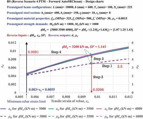
Design charts were developed based on Table 10 (Reverse Scenario 4) for three design moments ($\varphi$M_n = 3000, 3500, and 4000 kN·m) and tensile rebar strains (ε_rt), which vary between 0.0055 and 0.012. Design charts shown in Figures 7–15 were constructed for SRC beam having the following design parameters: M_D = 1000 kN·m, M_L = 1000 kN·m, L = 10,000 mm, b = 600 mm, f_y = 500 MPa, f′_c = 30 MPa, b_s = 150 mm, h_s = 600 mm, t_f = 10 mm, t_w = 8 mm, f_yS = 325 MPa, X_s = 225 mm, and Y_s = 100 mm. Sequence of determining design parameters can be established by engineers according to their design needs. In Figure 7, the design moment ($\varphi$M_n) used as the input parameter for AutoSRCbeam is given by the left ordinate, while the error between the network prediction calculated in Box 1 of Table 10 and AutoSRCbeam input is given by the right ordinate, demonstrating that the good accuracy of the design moment ($\varphi$M_n) determined by reverse network is shown. All errors of design moment ($\varphi$M_n) were less than 4% with respect to the preassigned tensile rebar strains (ε_rt) between 0.0055 and 0.012. Figure 8 shows the accuracy of the tensile rebar strains (ε_rt) corresponding to a concrete strain of 0.003 when they are preassigned on an input side. The tensile rebar strain (ε_rt) calculated with AutoSRCbeam is given by the left ordinate, while the error between the network prediction calculated in Box 2 of Table 10 and AutoSRCbeam calculation is given by the right ordinate. The errors of the tensile rebar strains (ε_rt) with respect to all design moments ($\varphi$M_n = 3000, 3500, and 4000 kN⋅m) were in a range between −6% and 3% for ε_rt = 0.0055 to 0.012. Figure 9 shows an accuracy of a safety factor (SF) corresponding to a concrete strain of 0.003 when they are preassigned as input parameters. The maximum error of a safety factor (SF) was less than 4% with respect to all design moments ($\varphi$M_n = 3000, 3500, and 4000 kN⋅m) for ε_rt = 0.0055 to 0.012.

Figure 7. Verification of design moments ($\varphi$M_n).

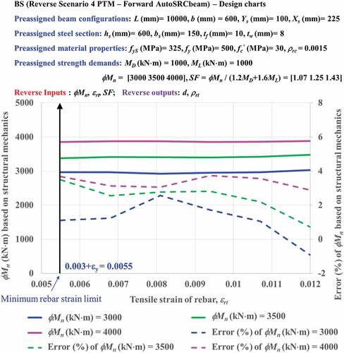
Figure 8. Verification of tensile rebar strain (ε_rt) corresponding to ε_c = 0.003.

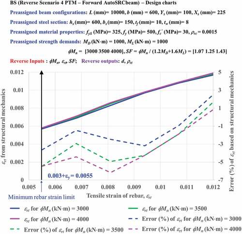
Figure 9. Verification of safety factor (SF) corresponding to ε_c = 0.003.

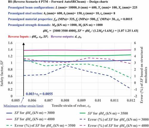
Figure 10. Design chart for determining d and ρ_rt as a function of tensile rebar strains (ε_rt) corresponding to a concrete strain of 0.003.

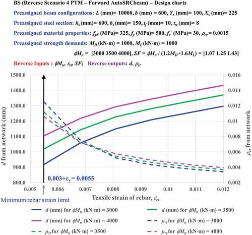
Figure 11. Design chart for determining ε_st and μ_$\varphi$ as a function of tensile rebar strains (ε_rt) corresponding to a concrete strain of 0.003.

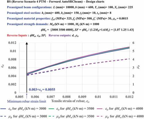
Figure 12. Design chart for determining ${\mathrm{\Delta }}_{imme}$ and ${\mathrm{\Delta }}_{long}$ as a function of tensile rebar strains (ε_rt) corresponding to a concrete strain of 0.003.

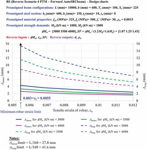
Figure 13. Design chart for determining CI_b and $C{O}_2\left(\mathrm{t}-\mathrm{C}{\mathrm{O}}_2\right)$ as a function of tensile rebar strains (ε_rt) corresponding to a concrete strain of 0.003.

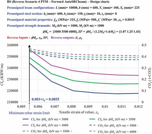
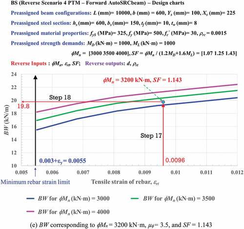
Figure 14. Design chart for determining BW as a function of tensile rebar strains (ε_rt) corresponding to a concrete strain of 0.003.

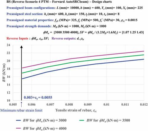
Figure 15. Design of an SRC beam using design charts.

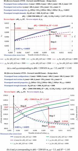
Figure 15. (Continued)

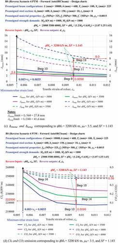
Figure 15. (Continued)

Figure 10 shows a relationship between effective depth (d) calculated in Box 17 of Table 10 and tensile rebar ratios (ρ_rt) calculated in Box 18 of Table 10 versus a tensile rebar strain (ε_rt) corresponding to a concrete strain of 0.003. Effective depth (d) is plotted in the direction opposite to a tensile rebar ratio (ρ_rt). Effective depth (d) increased with an increasing tensile rebar strain (ε_rt), but with a decreasing tensile rebar ratio (ρ_rt). Trends of effective depth (d) and tensile rebar ratio (ρ_rt) are shown with the opposite directions to keep stabilized with respect to design moments ($\varphi$M_n = 3000, 3500, and 4000 kN⋅m) as shown in Figure 10.

Figure 11 shows the tensile steel strain (ε_st) calculated in Box 19 of Table 10 and curvature ductility (μ_$\varphi$) calculated in Box 22 of Table 10 based on the varying tensile rebar strain (ε_rt) corresponding to a concrete strain of 0.003. The tensile steel strains (ε_st) increased almost linearly from 0.0045 to 0.011 with the tensile rebar strain between ε_rt = 0.0055 and 0.012 based on strain compatibility. Besides, a curvature ductility (μ_$\varphi$) increased from 2.15 to 4.08 for ε_rt = 0.0055 to 0.012, and they had clustered as shown in Figure 11.

Figure 12 shows the immediate and long-term deflections (${\mathrm{\Delta }}_{imme}$ calculated in Box 20 of Table 10 and ${\mathrm{\Delta }}_{long}$ calculated in Box 21 of Table 10) as functions of the tensile rebar strain (ε_rt) at a concrete strain of 0.003. An immediate deflection (${\mathrm{\Delta }}_{imme})$ decreased slightly between ε_rt = 0.0055 and 0.012 because the effect depth (d) shown in Figure 10 increased when the tensile rebar strain (ε_rt) increased from 0.005 to 0.015. However, when the tensile rebar strain (ε_rt) increased from 0.005 to 0.015, the long-term deflection (${\mathrm{\Delta }}_{long})$ decreased more significantly than the immediate deflection (${\mathrm{\Delta }}_{imme})$ because the effect of increased effective depth (d) shown in Figure 10 on the long-term deflection (${\mathrm{\Delta }}_{long})$ was less than that of the decreased compressive rebar ratios (ρ_rc) shown in Figure 10. In other words, the long-term deflection (${\mathrm{\Delta }}_{long})$ decreased even if the tensile rebar ratio (ρ_rt) shown in Figure 10 decreased, and the long-term effect factor was 1.86 (${\lambda }_D=2/\left(1+50\times {\rho }_{rc}\right)=1.86$).

As shown in Figure 13, the cost index of the beam (CI_b) calculated in Box 23 of Table 10 and CO₂ emissions calculated in Box 24 of Table 10 decreased as the tensile rebar strain (ε_rt) increased from 0.0055 to 0.012. This is because a tensile rebar ratio (ρ_rt) decreased (see Figure 10) even if an effective depth (d) increases. Cost index of a beam (CI_b) and CO₂ emission decreased rapidly when ε_rt = 0.0055–0.008. However, they decreased slightly when ε_rt = 0.008–0.012. This is because the tensile rebar ratio (ρ_rt) decreased rapidly when ε_rt = 0.0055–0.008 and slightly decreased when ε_rt = 0.008–0.012. A decrease in the tensile rebar ratio (ρ_rt) had a larger influence than an increase in effective depth (d) on a reduction of the amount of material cost to reduce the cost index (CI_b) and CO₂ emission as indicated in Figure 13. In Figure 14, a beam weight (BW) calculated in Box 25 of Table 10 increased rapidly when a tensile rebar strain (ε_rt) was from 0.0055 to 0.008 because effective depth (d) increased rapidly in this rebar strain range. However, beam weight (BW) increased gradually for ε_rt = 0.008 to 0.012 due to effective depth (d), which increased gradually in this rebar strain range. An increase in effective depth (d) causing more concrete volume to increase a beam weight (BW) had a greater influence than the decrease in the tensile rebar ratio (ρ_rt) on raising the concrete volume to increase the beam weight (BW).

5.4.3. Application of design charts

Figures 7–14 present graphical charts developed based on reverse designs shown in Table 10 comprising 10 output parameters (d, ρ_rt,ε_st,∆_imme,∆_long,µ_$\varphi$,CI_b, CO₂, BW, and X_s) and 16 input parameters ($\varphi$M_n,ε_rt, SF, L, b, f_y,f′_c,ρ_rc,h_s,b_s,t_f,t_w,f_yS,Y_s,M_D, and M_L). Design charts shown in Figures 9–14 assist engineers to design SRC beams. SRC beams can be designed when $\varphi$M_n,µ_$\varphi$, and SF are preassigned as input parameters on an input side. This type of design is challenging using conventional methods. Tensile rebar strain (ε_rt) and tensile steel strain (ε_st) were determined to be 0.0096 and 0.0091 for design moment ($\varphi$M_n) of 3200 kN·m, respectively, when a curvature ductility (μ_ɸ) was specified as 3.5 (Steps 1–4 in Figure 15(a)). The safety factor (SF) is selected as 1.143 for tensile rebar strain (ε_rt) of 0.0096 and design moment ($\varphi$M_n) of 3200 kN·m as shown in Figure 9, and hence, a safety factor (SF), curvature ductility (μ_ɸ), and design moment ($\varphi$M_n) of Figure 15 were set to 1.143, 3.5, and 3200 kN·m, respectively.

The effective depth (d) and tensile rebar ratio (ρ_rt) were determined to be 1247 mm and 0.0042, respectively, based on ε_rt = 0.0096 and design moment ($\varphi$M_n) of 3200 kN·m (Steps 5–8 in Figure 15(b)). The immediate deflection (∆_imme) of 2.60 mm and long-term deflection (∆_long) of 8.00 mm were then obtained (Steps 9–12 in Figure 15(c)). The cost index of the beam (CI_b) of 222,000 KRW/m, CO₂ emissions of 0.380 t-CO₂/m, and beam weight (BW) of 19.80 kN/m were then obtained (Steps 13–18 in Figures 15(d and e). Figure 16 summarizes the design of an SRC beam with preassigned $\varphi$M_n = 3200 kN·m, µ_$\varphi$ = 3.5 and SF = 1.143. Section A–A was determined based on the AI-based reverse design charts, which shows an immediate deflection of 2.80 mm and long-term deflection of 8.00 mm. These values are less than the design limits of 27.8 (L/360) and 41.6 mm (L/240), respectively. CI_b, CO₂ emissions, and BW were also obtained, which can help engineers with making the final design decisions. Table 11 presents the validated results of AI-based graphical design for a SRC beam section corresponding to $\varphi$M_n = 3200 kN·m, µ_$\varphi$ = 3.5, and SF = 1.143, which is challenging to perform with conventional methods. A maximum error of −2.08% was obtained for the tensile strain of rebar (ε_rt) based on structural mechanics. An acceptable accuracy was obtained for most of the other design parameters.

Figure 16. Procedure to design SRC beams with preassigned parameters [ɸM_n = 3200 kN·m, μ_ɸ = 3.5, SF = 1.143, M_D = 1000 kN·m, M_L = 1000 kN·m, L = 10,000 mm, b = 600 mm, f_y = 500 MPa, f_c’ = 30 MPa, b_s = 150 mm, h_s = 600 mm, t_f = 10 mm, t_w = 8 mm, f_yS = 325 MPa, X_s = 225 mm, Y_s = 100 mm].

Table 11. Verification of reverse design for SRC beam sections corresponding to ɸM_n = 3200 kN·m, µ_ɸ = 3.5.

6. Conclusions

In this study, an ANN was applied to the design of SRC beams, which can be a lengthy process because understanding how parameters influence one another are difficult. The objective was to develop an AI-based design method for SRC beams, which can have over 25 design parameters. Reverse designs were obtained by training ANNs with large datasets and mapping input to output parameters rather than through structural mechanics or knowledge. Fast and accurate reverse design of SRC members is now possible when the calculation sequences of inputs and outputs are exchanged. The accuracy was verified through structural calculations using conventional methods. The following recommendations are suggested for the fast and accurate design of SRC beams.

(1) Artificial intelligence-based reverse design charts are generated for rapid and accurate designing of SRC members even when the calculation sequences of the input and output parameters are exchanged, which is challenging to achieve with conventional design methods. ANNs are trained on multiple nonlinear inputs and output parameters. The developed network is capable of designing SRC beams with various scenarios by accurately determining design parameters for given unseen structural input parameters.

(2) An AI-based reverse design method is presented with applicable design charts when the calculation sequences of inputs and outputs are arbitrarily selected. The network accuracy for the SRC design was verified through structural calculations with the conventional method. The ANN showed extrapolation with limited accuracies when input conflicts were avoided, even if the inputs and outputs lay outside the training datasets. However, the network accuracy became weak in general with input conflicts when applied to values outside the training datasets.

(3) Direct and BS methods are implemented. In the BS method, a training takes two steps, where input parameters for a forward network of Step 2 are calculated as reverse outputs of a network of Step 1 for given reverse input parameters. Reverse output parameters of Step 1 are, then, substituted as input parameters of Step 2 to obtain design parameters.

(4) Design charts are provided for practical application to SRC beams. They enable the fast and accurate determination of design parameters for both forward and reverse designs. The design charts can assist engineers with obtaining preliminary designs for SRC beams by predicting multiple design parameters in any order.

(5) Robust design of SRC beams based on design charts is now possible, which is challenging to achieve with conventional design methods. Reverse techniques can be implemented in many areas of design.

(6) Artificial intelligence-based reverse design charts were generated for rapid and accurate designing of SRC members even when the calculation sequences of the input and output parameters were exchanged, which is challenging to achieve with conventional design methods.

(7) Reverse deign can pose an input conflict when pre-assigned input parameters are not well selected, preventing AI-based design from being practical for engineers. Next study will identify optimized parameters in forward manner to avoid and input conflicts, based on Lagrange optimization with equality and inequality conditions.

(8) Big data must be generated according to well-known design codes such as ACI, EC, KDS, etc., for real-world applications, and hence, the present study derives ANN-based design charts for SRC beams based on the latest American standards (ACI 318–19), being applicable in many countries. Contributions of steel, concrete, rebars, and stirrups to stiffnesses and strengths are well described in many design codes such as ACI, EC, KDS, etc., and hence, data generations for SRC beams are not complex once code-based manuals are followed. ANN-based design charts prepared based on AI-based flowchart described in Sections 4 and 5 of this study can be conveniently remade for different design codes available.

Nomenclature

Forward parameters

L (mm)	=	Beam length
d (mm)	=	Effective beam depth
b (mm)	=	Beam width
f’c (MPa)	=	Compressive concrete strength
fy (MPa)	=	Yield rebar strength
ρrt	=	Tensile rebar ratio
ρrc	=	Compressive rebar ratio
hs (mm)	=	H-shaped steel height
bs (mm)	=	H-shaped steel width
tf (mm)	=	H-shaped steel flange thickness
tw (mm)	=	H-shaped steel web thickness
fyS (MPa)	=	Yield steel strength
Ys (mm)	=	Clearance between H steel section and closest rebar layer
MD (kN·m)	=	Moment due to dead load
ML (kN·m)	=	Moment due to live load

Reverse parameters

ΦMn (kN·m)	=	Design moment without considering effect of self-weight at εc = 0.003
εrt	=	Tensile rebar strain at εc = 0.003
εst	=	Strain of tensile steel flange at εc = 0.003
Δimme (mm)	=	Immediate deflection due to live load, ML
Δlong (mm)	=	Sum of time-dependent deflection due to sustained loads and immediate deflection due to any additional live load
µΦ	=	Curvature ductility
CIb (KRW/m)	=	Cost index per 1m length of beam
CO2 (t-CO2/m)	=	CO2 emission per 1m length of beam
BW (kN/m)	=	Beam weight per 1m length of beam
Xs (mm)	=	Clearance between flange of H steel section and edge of beam
SF	=	Safety factor

Acknowledgments

This work was supported by a National Research Foundation of Korea (NRF) grant funded by the Korean government (MSIT 2019R1A2C2004965).

Disclosure statement

No potential conflict of interest was reported by the author(s).

Correction Statement

This article has been republished with minor changes. These changes do not impact the academic content of the article.

Additional information

Funding

This work was supported by the National Research Foundation of Korea (NRF) grant funded by the Korean government [MSIT 2019R1A2C2004965].

Notes on contributors

Won-Kee Hong

Dr. Won-Kee Hong is a Professor of Architectural Engineering at Kyung Hee University. Dr. Hong received his Master’s and Ph.D. degrees from UCLA, and he worked for Englelkirk and Hart, Inc. (USA), Nihhon Sekkei (Japan) and Samsung Engineering and Construction Company (Korea) before joining Kyung Hee University (Korea). He also has professional engineering licenses from both Korea and the USA. Dr. Hong has more than 30 years of professional experience in structural engineering. His research interests include a new approach to construction technologies based on value engineering with hybrid composite structures. He has provided many useful solutions to issues in current structural design and construction technologies as a result of his research that combines structural engineering with construction technologies. He is the author of numerous papers and patents both in Korea and the USA. Currently, Dr. Hong is developing new connections that can be used with various types of frames including hybrid steel–concrete precast composite frames, precast frames and steel frames. These connections would help enable the modular construction of heavy plant structures and buildings. He recently published a book titled as ”Hybrid Composite Precast Systems: Numerical Investigation to Construction” (Elsevier).

Dinh Han Nguyen

Dinh Han Nguyen is a Postdoctoral researcher in the Department of Architectural Engineering at Kyung Hee University, Republic of Korea. His research interest includes precast structures.

Van Tien Nguyen

Van Tien Nguyen is currently enrolled as a Master's candidate in the Department of Architectural Engineering at Kyung Hee University, Republic of Korea. His research interest includes precast structures.

References

- Adeli, H. 2001. “Neural Networks in Civil Engineering: 1989–2000.” Computer Aided Civil and Infrastructure Engineering 16 (2): 126–142. doi:10.1111/0885-9507.00219.
- Adeli, H., and H. S. Park. 1995a. “A Neural Dynamics Model for Structural optimization—theory.” Computers & Structures 57 (3): 383–390. doi:10.1016/0045-7949(95)00048-L.
- Adeli, H., and H. S. Park. 1995b. “Optimization of Space Structures by Neural Dynamics.” Neural Networks 8 (5): 769–781. doi:10.1016/0893-6080(95)00026-V.
- Asteris, P. G., S. Nozhati, M. Nikoo, L. Cavaleri, and M. Nikoo. 2019. “Krill Herd algorithm-based Neural Network in Structural Seismic Reliability Evaluation.” Mechanics of Advanced Materials and Structures 26 (13): 1146–1153. doi:10.1080/15376494.2018.1430874.
- Berrais, A. 1999. “Artificial Neural Networks in Structural Engineering: Concept and Applications.” Engineering Sciences 12 (1): 53-67.
- Chan, W. T., Y. K. Chow, and L. F. Liu. 1995. “Neural Network: An Alternative to Pile Driving Formulas.” Computers and Geotechnics 17 (2): 135–156. doi:10.1016/0266-352X(95)93866-H.
- Das, S. K., and P. K. Basudhar. 2006. “Undrained Lateral Load Capacity of Piles in Clay Using Artificial Neural Network.” Computers and Geotechnics 33 (8): 454–459. doi:10.1016/j.compgeo.2006.08.006.
- Fahmy, A. S., M. E. T. El-Madawy, and Y. A. Gobran. 2016. “Using Artificial Neural Networks in the Design of Orthotropic Bridge Decks.” Alexandria Engineering Journal 55 (4): 3195–3203. doi:10.1016/j.aej.2016.06.034.
- Flood, I., and N. Kartam. 1994a. “Neural Networks in Civil Engineering. I: Principles and Understanding.” Journal of Computing in Civil Engineering 8 (2): 131–148. doi:10.1061/(ASCE)0887-3801.
- Flood, I., and N. Kartam. 1994b. “Neural Networks in Civil Engineering. II: Systems and Application.” Journal of Computing in Civil Engineering 8 (2): 149–162. doi:10.1061/(ASCE)0887-3801.
- Gupta, T., and R. K. Sharma. 2011. “Structural Analysis and Design of Buildings Using Neural Network: A Review.” International Journal of Engineering and Management Sciences 2 (4): 216–220.
- Hajela, P., and L. Berke. 1991. “Neurobiological Computational Models in Structural Analysis and Design.” Computers & Structures 41 (4): 657–667. doi:10.1016/0045-7949(91)90178-O.
- Hanna, A. M., G. Morcous, and M. Helmy. 2004. “Efficiency of Pile Groups Installed in Cohesionless Soil Using Artificial Neural Networks.” Canadian Geotechnical Journal 41 (6): 1241–1249. doi:10.1139/t04-050.
- Hong, W. K. 2019. Hybrid Composite Precast Systems: Numerical Investigation to Construction. Woodhead Publishing, Elsevier.
- Hong, W. K. 2021. Artificial intelligence-based Design of Reinforced Concrete Structures. Daega.
- Hong, W. K. 2023. “Artificial Neural Network-based Optimized Design of Reinforced Concrete structures, Tayor & Francis Group.” [Under preparation]
- Hong, W. K., J. M. Kim, S. C. Park, S. G. Lee, S. I. Kim, K. J. Yoon, H. C. Kim, and J. T. Kim. 2010. “A New Apartment Construction Technology with Effective CO2 Emission Reduction Capabilities.” Energy 35 (6): 2639–2646. doi:10.1016/j.energy.2009.05.036.
- Hong, W. K., T. A. Le, M. C. Nguyen, and T. D. Pham. 2022. “ANN-based Lagrange Optimization for RC Circular Columns Having multi-objective Functions.” Journal of Asian Architecture and Building Engineering 1–16. doi:10.1080/13467581.2022.2064864. accepted
- Hong, W. K., and M. C. Nguyen. 2021. “AI-based Lagrange Optimization for Designing Reinforced Concrete Columns.” Journal of Asian Architecture and Building Engineering. doi:10.1080/13467581.2021.1971998.
- Hong, W. K., V. T. Nguyen, and M. C. Nguyen. 2021. “Artificial Intelligence-based Novel Design Charts for Doubly Reinforced Concrete Beams.” Journal of Asian Architecture and Building Engineering. doi:10.1080/13467581.2021.1928511.
- Hong, W. K., V. T. Nguyen, and M. C. Nguyen. 2021. “Optimizing Reinforced Concrete Beams Cost Based on AI-based Lagrange Functions.” Journal of Asian Architecture and Building Engineering 1–18.
- Hong, W. K., V. T. Nguyen, D. H. Nguyen, and M. C. Nguyen. 2022a. “An AI-based Lagrange Optimization for a Design for Concrete Columns Encasing H-Shaped Steel Sections under a Biaxial Bending.” Journal of Asian Architecture and Building Engineering accepted.
- Hong, W. K., V. T. Nguyen, D. H. Nguyen, and M. C. Nguyen. 2022b. “Reverse design-based Optimizations for Reinforced Concrete Columns Encasing H-shaped Steel Section Using ANNs.” Journal of Asian Architecture and Building Engineering 1–15 .
- Hong, W. K., M. C. Nguyen, and T. D. Pham. 2022. “Optimized Interaction PM Diagram for Rectangular Reinforced Concrete Column Based on Artificial Neural Networks Abstract.” Journal of Asian Architecture and Building Engineering 1–25. doi:10.1080/13467581.2021.2018697.
- Hong, W. K., and T. D. Pham. 2021. “Reverse Designs of Doubly Reinforced Concrete Beams Using Gaussian Process Regression Models Enhanced by Sequence Training/Designing Technique Based on Feature Selection Algorithms.” Journal of Asian Architecture and Building Engineering 1–26. doi:10.1080/13467581.2021.1971999.
- Hong, W. K., T. D. Pham, and V. T. Nguyen. 2021. “Feature Selection Based Reverse Design of Doubly Reinforced Concrete Beams.” Journal of Asian Architecture and Building Engineering 1–26. doi:10.1080/13467581.2021.1928510.
- Huang, C., and S. Huang.2020.“Predicting Capacity Model and Seismic Fragility Estimation for RC Bridge Based on Artificial Neural Network.” In Structures, 1930–1939. Elsevier. Vol. 27. doi:10.1016/j.istruc.2020.07.063.
- Kang, H. T., and C. J. Yoon. 1994. “Neural Network Approaches to Aid Simple Truss Design Problems.” Computer Aided Civil and Infrastructure Engineering 9 (3): 211–218. doi:10.1111/j.1467-8667.1994.tb00374.x.
- Lagaros, N. D., and M. Papadrakakis. 2012. “Neural Network Based Prediction Schemes of the non-linear Seismic Response of 3D Buildings.” Advances in Engineering Software 44 (1): 92–115. doi:10.1016/j.advengsoft.2011.05.033.
- Lavaei, A., and A. Lohrasbi “Dynamic Analysis of Structures Using Neural Networks.” The 15th World Conference on Earthquake Engineering 2012, Lisbon, Portugal
- Lee, S., J. Ha, M. Zokhirova, H. Moon, and J. Lee. 2018. “Background Information of Deep Learning for Structural Engineering.” Archives of Computational Methods in Engineering 25 (1): 121–129. doi:10.1007/s11831-017-9237-0.
- Lee, I. M., and J. H. Lee. 1996. “Prediction of Pile Bearing Capacity Using Artificial Neural Networks.” Computers and Geotechnics 18 (3): 189–200. doi:10.1016/0266-352X(95)00027-8.
- Lee, C., and R. Sterling. 1992. “Identifying Probable Failure Modes for Underground Openings Using a Neural Network.” International Journal of Rock Mechanics and Mining Sciences & Geomechanics Abstracts 29 (1): 49–67. Pergamon doi:10.1016/0148-9062(92)91044-6
- MathWorks, (2022a). Deep Learning Toolbox: User’s Guide (R2022a). Retrieved July 26, 20122 from: https://www.mathworks.com/help/pdf_doc/deeplearning/nnet_ug.pdf
- MathWorks, (2022a). Parallel Computing Toolbox: Documentation (R2022a). Retrieved July 26, 2022 from: https://uk.mathworks.com/help/parallel-computing/
- MathWorks, (2022a). Statistics and Machine Learning Toolbox: Documentation (R2022a). Retrieved July 26, 2022 from: https://uk.mathworks.com/help/stats/
- MathWorks, (2022a). MATLAB (R2022a).
- Neaupane, K., and S. Achet. 2004. “Some Applications of a Backpropagation Neural Network in geo-engineering.” Environmental Geology 45 (4): 567–575. doi:10.1007/s00254-003-0912-0.
- Nguyen, D. H. “Artificial Intelligence (Ai)-based Design Methodology for steel-reinforced Concrete (SRC) Members.” Ph.D. dissertation, Kyung Hee University 2021.
- Nguyen, D. H., and W. K. Hong. 2019. “Part I: The Analytical Model Predicting post-yield Behavior of concrete-encased Steel Beams considering Various Confinement Effects by Transverse Reinforcements and Steels.” Materials 12 (14): 2302. doi:10.3390/ma12142302.
- Oh, B. K., B. Glisic, S. W. Park, and H. S. Park. 2020. “Neural network-based Seismic Response Prediction Model for Building Structures Using Artificial Earthquakes.” Journal of Sound and Vibration 468: 115109. doi:10.1016/j.jsv.2019.115109.
- Pham, T. D., and W. K. Hong. 2022. “Genetic Algorithm Using probabilistic-based Natural Selections and Dynamic Mutation Ranges in Optimizing Precast Beams.” Computers & Structures 258: 106681. doi:10.1016/j.compstruc.2021.106681.
- Rahman, M. S., J. Wang, W. Deng, and J. P. Carter. 2001. “A Neural Network Model for the Uplift Capacity of Suction Caissons.” Computers and Geotechnics 28 (4): 269–287. doi:10.1016/S0266-352X(00)00033-1.
- Shi, J. J. 2003. “Reducing Prediction Error by Transforming Input Data for Neural Networks.” Journal of Computing in Civil Engineering 14 (2): 109–116. doi:10.1061/(ASCE)0887-3801(2000).
- Shi, J., J. A. R. Ortigao, and J. Bai. 1998. “Modular Neural Networks for Predicting Settlements during Tunneling.” Journal of Geotechnical and Geoenvironmental Engineering 124 (5): 389–395. doi:10.1061/(ASCE)1090-0241.
- Tashakori, A., and H. Adeli. 2002. “Optimum Design of cold-formed Steel Space Structures Using Neural Dynamics Model.” Journal of Constructional Steel Research 58 (12): 1545–1566. doi:10.1016/S0143-974X(01)00105-5.
- Vanluchene, R. D., and R. Sun. 1990. “Neural Networks in Structural Engineering.” Computer Aided Civil and Infrastructure Engineering 5 (3): 207–215. doi:10.1111/j.1467-8667.1990.tb00377.x.
- Wu, R. T., and M. R. Jahanshahi. 2019. “Deep Convolutional Neural Network for Structural Dynamic Response Estimation and System Identification.” Journal of Engineering Mechanics 145 (1): 04018125. doi:10.1061/(ASCE)EM.1943-7889.0001556.
- Ying, W., W. Chong, L. Hui, and Z. Renda “Artificial Neural Network Prediction for Seismic Response of Bridge Structure.” International Conference on Artificial Intelligence and Computational Intelligence. Shanghai, China. 2009 (Vol. 2, pp. 503–506). IEEE. DOI: 10.1109/AICI.2009.303
- Yoo, C., and J. M. Kim. 2007. “Tunneling Performance Prediction Using an Integrated GIS and Neural Network.” Computers and Geotechnics 34 (1): 19–30. doi:10.1016/j.compgeo.2006.08.007.