Holistic design of pre-tensioned concrete beams based on Artificial Intelligence

ABSTRACT

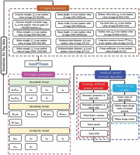
This research demonstrates how pre-tensioned concrete beams (PT beams) are designed holistically using artificial neural networks (ANNs). To establish reverse design scenarios, large input and output data are generated using the mechanics-based software AutoPTbeam. ANN-trained reverse-forward networks are proposed to solve reverse designs with 15 input and 18 output parameters for engineers. ANNs for reverse designs pre-tensioned concrete beams are formulated based on 15 input structural parameters to investigate the performances of PT beams with pin-pin boundaries. Useful reverse designs based on neural networks can be established by relocating preferable control parameters on an input-side, such as when four output parameters ($q_{L/250,}{q}_{0.2mm,}{q}_{str,}{\mu }_{\mathrm{\Delta }}$) (reverse scenario) are reversely pre-assigned on an input-side, all associated design parameters, including crack width, rebar strains at transfer load stage, rebar strains, and displacement ductility ratio at ultimate load stage are computed on an output-side. Deep neural networks trained by chained training scheme with revised sequence (CRS) for the reverse network of Step 1 show the better design accuracies when compared to those obtained based on ANNs trained by parallel training method (PTM) and based on shallow neural networks trained by CRS when the deflection ductility ratios (μ_Δ) within generated big datasets are reversely pre-assigned on an input-side.

GRAPHICAL ABSTRACT

KEYWORDS:

• Artificial intelligence
• pre-tensioned beams
• reverse designs
• design chart
• curvature ductility

1. Introduction

1.1. Previous studies

Several artificial neural network-based studies of prestressed beams have been conducted. Torky and Aburawwash (Torky and Aburawwash 2018) published a simple prestressed beam to demonstrate the viability of neural networks over traditional approaches. They proposed a deep learning approach to optimizing prestressed beams. Their data, however, are limited to beam depth, beam width, bending moment, eccentricity, and a number of strands.

Sumangala and Jeyasehar (Sumangala and Antony Jeyasehar 2011) also studied a damage assessment procedure using an artificial neural network (ANN) for prestressed concrete beams. They formulated the methodology using the results obtained from an experimental study conducted in the laboratory. The measured output from both static and dynamic tests was taken as input to train the neural network based on MATLAB. The quantitative evaluation of the degree of damage was possible by ANN using the natural frequency and stiffness in the post-cracking range. Their damage assessment procedure was validated using the data available in the literature, and the outcome is presented in Sumangala and Antony Jeyasehar (2011). Lee et al. (2019) proposed a novelty detection approach for tendons of PSC bridges based on a convolutional autoencoder (CAE). The proposed method used simulation data from nine different accelerometers. According to their research, the accuracies of CAEs for multi-vehicle are 79.5%–85.8% for 100% and 75% damage severities. Sanqiang Yang and Yong Huang also (Yang and Huang 2021) identified damages of prestressed concrete beam bridge based on a convolutional neural network. An additional study has been performed by (Alhassan, Ababneh, and Betoush 2020) who studied an innovative model for accurate prediction of the transfer length of prestressing strands based on artificial neural networks. Tam et al. (2004) also diagnosed prestressed concrete pile defects using probabilistic neural networks. Mo and Han (1995) investigated prestressed concrete frame behavior with neural networks. Slowik, Lehký, and Novák (2021) investigated reliability-based optimization of a prestressed concrete roof girder using a surrogate model and the double-loop approach, while Khandel et al. (2021) used a statistical damage detection and localization approach to evaluate the performance of prestressed concrete bridge girders using fiber Bragg grating sensors based on artificial neural networks. Roya (Solhmirzaei et al. 2020) investigated 360 test results ultra high performance concrete beams using different machine learning algorithms, resulting in good accuracies in predicting beam failure mode and shear capacity.

However, these studies are not dedicated to a holistic design of prestressed beams for practical applications. In the current study, both forward and reverse designs for prestressed beams are possible, with real-world big datasets of 50,000 generated using the full scale of structural mechanics-based software and trained using their previous training methods shown below. Hong, Pham, and Nguyen (2021) proposed training methods based on a feature selection for a reverse design of doubly reinforced concrete beams. They trained large datasets using TED, PTM, CTS, and CRS that they developed. Hong et al. also presented artificial intelligence-based novel design charts for doubly reinforced concrete beams (Hong, Nguyen, and Nguyen 2021) and novel design methods for reinforced concrete columns (Hong, Nguyen, and Pham 2022). Hong and Pham (2021) performed reverse designs of doubly reinforced concrete beams using Gaussian process regression models enhanced by sequence training/designing techniques based on feature selection algorithms. The training methods developed in Hong, Pham, and Nguyen (2021), Hong, Nguyen, and Nguyen (2021) Hong, Nguyen, and Pham (2022), and Hong and Pham (2021) are used to map 15 input parameters to 18 output parameters for a holistic design of pre-tensioned concrete beams. The large datasets, which contain 33 parameters, including 15 input and 18 output parameters, aid in the accurate training of ANNs that represent prestressed beams.

1.2. Research significance

There are numerous available computer-aided engineering tools, including CAD packages, FEM software, self-written calculation codes, that are used to study the performance of the PT structures. In this study, ANNsprogramed based on MATLAB Deep Learning Toolbox (MathWorks 2022a), MATLAB Parallel Computing Toolbox (MathWorks 2022b), MATLAB Statistics and Machine Learning Toolbox (MathWorks 2022c), and MATLAB R2022a (MathWorks) are used to design PT structures based on EC2 2004 (CEN (European Committee for Standardization) 2004) in both forward and reverse directions. When big data is good enough to show a tendency of PT beam behaviors, a reverse solution is generalizable by using ANNs trained on big data. Based on large datasets, forward and reverse designs using ANNs are possible, with no need for primary engineering knowledge to effectively determine design parameters for practices. The proposed networks allow for both forward and reverse designs for PT beams, which is difficult to achieve with classic techniques. AI-based PT beam design with sufficient training accuracy can completely replace classical design software while exhibiting excellent productivity for both forward and reverse designs. To better demonstrate the design steps, numerical examples are provided. Design charts are also constructed for design scenarios. Design charts can be extended as further as possible to meet the requirements of engineers.

The proposed method is advantageous in that it is less dependent on problem types such as column, beam, frame, seismic design, and so on, and instead relies on characteristics of large datasets of the considered problem. As a result, the proposed method’s applications are not limited to designing PT beams but can also be extended to other structures.

2. Formulations of forward design; description of input and output parameters

2.1. Description of input parameters

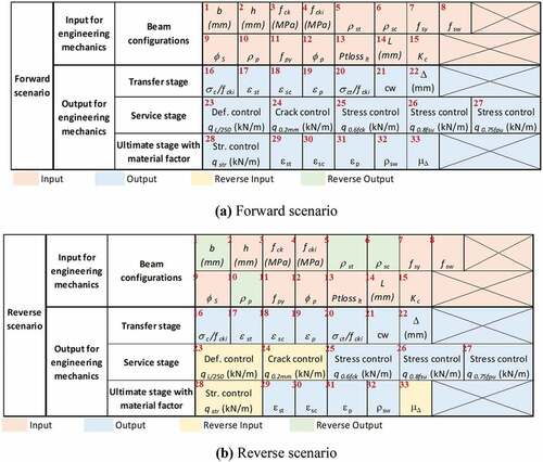
ANNs are implemented in designing bonded pre-tensioned beams with pin-pin ends shown in Figure 1, illustrating beam width (mm) b, beam depth (mm) h, and beam length (mm) L. Table 1 presents fifteen input parameters to generate big datasets using AutoPTbeam for an AI-based reverse design. Concrete properties include compressive cylinder strength of concrete at 28 days (MPa, f_ck), compressive cylinder strength of concrete at transfer stage (MPa, f_cki), and long-term deflection factor considering creep effect, (normally 2.5 ~ 3.5, K_c). Reinforcing bar properties include top, bottom rebar ratios (ρ_st and ρ_sc), yield stress of rebar (MPa, f_sy), yield stress of stirrup (MPa, f_sw), and preferred diameter (mm, ${\varphi }_s$). Tendon properties include tendon ratios (ρ_p), yield stress (MPa, f_py), and preferred diameter (mm, ${\varphi }_p$). Long-term pre-stress losses (PTLoss_lt) is also one of fifteen input parameters. Tensile strength of tendon f_pu is set as 1860 MPa, and hence, f_pu is not included in inputs of big datasets.

Figure 1. Bonded pre-tensioned beams with pin-pin ends for an AI-based design.

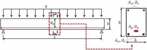
Table 1. Fifteen input parameters to generate big datasets using AutoPTbeam for pre-tensioned beams.

15 INPUTS
No	Symbol	Definition	No	Symbol	Definition
1	$b$	Beam width (mm)	9	${\varphi }_s$	Preferred rebar diameter (mm)
2	$h$	Beam depth (mm)	10	$\rho p$	Tendon ratio
3	$fck$	Concrete strength (MPa)	11	$fpy$	Yielding stress of tendon (MPa)
4	$fck$	Concrete strength at transfer stage (MPa)	12	$\varphi P$	Preferred tendon diameter (mm)
5	$\rho st$	Bottom rebar ratio	13	$PTlosslt$	Long-term prestress losses
6	$\rho sc$	Top rebar ratio	14	$L$	Beam length (mm)
7	$fsy$	Yielding stress of rebar (MPa)	15	$Kc$	Creep coefficient
8	$fsw$	Yielding stress of stirrup (MPa)

2.2. Description of output parameters

There are three load stages considered in prestressed designs, as shown in Figure 2. The present study investigates 18 output parameters, including seven output parameters at the transfer load stage, five output parameters at the service load limit stages, and six outputs at the ultimate load limit stage, respectively, as shown in Table 2.

Figure 2. Three load stages of PT beams.

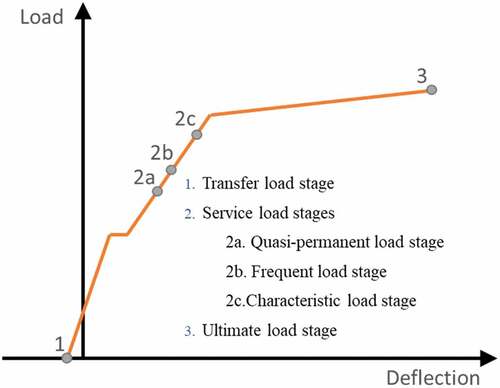
Table 2. 18 output of forward designs of a PT beam.

(a) Seven outputs at transfer load stages
No	Symbol	Definition
1	$\sigma c/fcki$	Top concrete stress per concrete strength at transfer stage
2	$\epsilon st$	Bottom rebar strain at transfer stage
3	$\epsilon sc$	Top rebar strain at transfer stage
4	$\epsilon p$	Tendon strain at transfer stage
5	$\sigma ct/fcki$	Bottom concrete stress per concrete strength at transfer stage
6	$cw$	Crack width at transfer stage
7	$\mathrm{\Delta }$	Defection at transfer stage
(b) Five output parameters at service load limit stage (Quasi, frequent, characteristic)
8	$qL/250$	Nominal strength when deflection reaches to L/250
9	$q0.2mm$	Nominal strength when crack width reaches to 0.2 mm
10	$q0.6fck$	Nominal strength when concrete stress reaches to stress limitation ($0.6f_{ck}$)
11	$q0.8fsu$	Nominal strength when rebar stress reaches to stress limitation ($min\left[0.8f_{su};f_{sy}\right])$
12	$q0.75fpu$	Nominal strength when tendon stress reaches to stress limitation ($min\left[0.75f_{pu};f_{py}\right]$)
(c) Six output parameters at ultimate load limit stage, considering both strength and ductility of member
13	$qstr$	Maximum nominal strength that a PT beam
14	$\epsilon st$	Bottom rebar strain at ultimate stage
15	$\epsilon sc$	Top rebar strain at ultimate stage
16	$\epsilon p$	Tendon strain at ultimate stage
17	$\rho sw$	Stirrup ratio
18	${\mu }_{\Delta }$	Deflection ductility

Table 2(a) illustrates seven outputs of forward designs at a transverse stage, where EC 2 (CEN (European Committee for Standardization) 2004) requires concrete compressive stress (${\sigma }_c$) to be smaller than $0.6f_{cki}$, crack widths to be under a limitation depending on environmental condititons, and top rebar stress (${\sigma }_{sc}$) to be less than a smaller number between $0.8f_{su}\mathrm{a}\mathrm{n}\mathrm{d}{f}_{sy}$. It is noted that, EC2 (CEN (European Committee for Standardization) 2004) determines crack limitations using six classes of environmental exposures, which are classified based on a risk of being attacked by carbonation-induced corrosion, chloride-induced corrosion, freeze thaw, or chemicals.

Table 2(b) shows five nominal strengths, corresponding to maximum applied loads on beams without violating service limitations required by EC2 (CEN (European Committee for Standardization) 2004). There are three sub-stages named quasi-permanent, frequent, and characteristic in a service load stage, where EC2 (CEN (European Committee for Standardization) 2004) requires PT beams to satisfy five design limitations. First of all, deflections should not exceed a limitation of L/250 at a quasi-permanent load stage. Secondly, crack widths under frequent load combinations should not exceed a limitation (Uncrack, 0.1 mm, 0.2 mm or 0.4 mm, etc.). Thirdly, concrete compressive stresses (${\sigma }_c$) under characteristic load combinations should be smaller than $0.6f_{ck}$ to avoid longitudinal cracks. Finally, rebar stresses are limited at a minimum of $0.8f_{su}$ and $f_{sy}$, whereas tendon stresses (${\sigma }_P$) should not exceed a smaller number between $0.75f_{pu}$ and $f_{py}$ to avoid unacceptable cracks or deformations at characteristic load combinations.

Table 2(c) presents six outputs of forward designs at ultimate stages. AutoPTbeam calculates maximum nominal strength, rebar strains, tendon strains, and deflection ductility at ultimate stage, providing a clear insight into structural behaviors under fracture loads.

Tables 1 and 2 summarizes all the 33 input and output parameters used for generating large datasets for training ANNs. The large datasets are used for AI-based design for both forward (Section 4) and reverse designs (Section 5) of simply supported bonded pre-tensioned beams for all stages.

2.3. Generation of large structural datasets and network training

Table 3 and Figures 3-6 contain a list of random variables, their corresponding ranges, and data distributions from the large structural datasets. The algorithm of AutoPTbeam shown in Figure 7(a) was developed for designing the forward design of bonded pre-tensioned beams by Cuong and Hong (Nguyen and Hong 2021). Figure 7(b) shows flow charts for generating large structural datasets for training ANNs. Table 7(b) displays large structural datasets with selected non-normalized fifteen inputs and eighteen outputs generated based on Figure 7(b).

Figure 3. Histogram of 15 inputs based on 50.000 data.

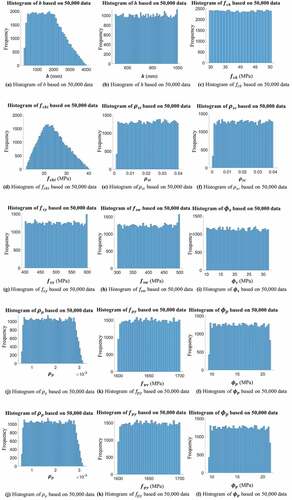
Figure 4. Histogram of seven outputs of a transfer stage based on 50.000 data.

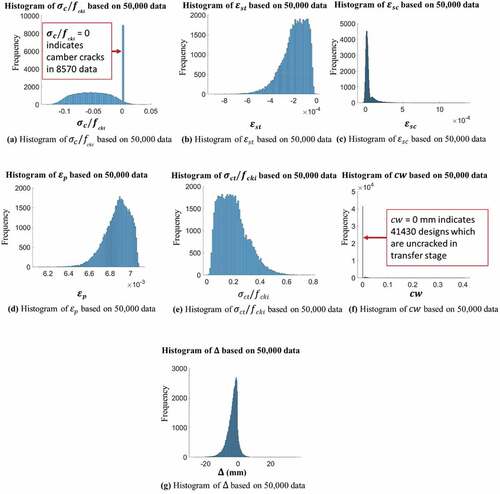
Figure 5. Histogram of five outputs of a service stage based on 50.000 data.

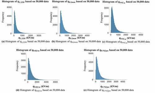
Figure 6. Histogram of six outputs of an ultimate stage based on 50.000 data (a) Algorithm for designing bonded pre-tensioned beams (AutoPTbeam) (b) Generation of large datasets.

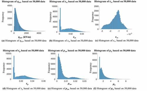
Figure 7. Generation of large datasets of bonded pre-tensioned beams for AI-based design (Nguyen and Hong 2021)

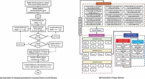
Table 3. List of random variables and corresponding ranges of the big structural datasets.

(a) Big datasets for bonded pre-tensioned beams; non-normalized fifteen inputs
	$b\left(mm\right)$	$h\left(mm\right)$	$f_{ck}\hspace{0.17em}\left(MPa\right)$	$f_{cki\left(MPa\right)}$	${\rho }_{st}$	${\rho }_{sc}$	$f_{sy\left(MPa\right)}$	$f_{sw}\left(Mpa\right)$
Large data	555.27	837	45	33.43	0.0300	0.0225	447	329
	1034.07	646	44	26.11	0.0199	0.0214	524	341
	395.70	893	42	20.70	0.0329	0.0106	545	322
	2970.61	980	35	23.94	0.0148	0.0174	526	486
	…
MAX	3977.23	1000	50	40.00	0.0400	0.0400	600	500
MIN	203.58	500	30	12.00	0.0012	0.0005	400	300
MEAN	1645.86	749.84	40.04	23.97	0.0208	0.0203	499.46	400.11
STANDARD DEVIATION	857.44	144.67	6.07	5.92	0.0110	0.0113	57.99	58.27
VARIANCE	735210.02	20,931.70	36.89	35.03	0.0001	0.0001	3363.86	3396.45
	${\varphi }_s$	${\rho }_p$	$f_{py\left(MPa\right)}\hspace{0.17em}$	${\varphi }_p$	$PTlos{s}_{lt}$	$L\left(mm\right)$	$K_c$
Large data	29	0.0020	1693	20.2	0.11	14,224	3.28
	22	0.0012	1662	19.5	0.16	12,262	2.93
	14	0.0024	1600	10.7	0.14	9115	2.94
	25	0.0028	1615	18.2	0.14	11,109	2.88
	…
MAX	32	0.0032	1700	21.5	0.20	19,892	3.50
MIN	10	0.0006	1600	9.5	0.10	4058	2.50
MEAN	21	0.0018	1650.08	15.5	0.15	10,476	3.00
STANDARD DEVIATION	6.35	0.0006	28.98	3.4	0.029	3332	0.288
VARIANCE	40.41	4.7675	839.88	11.9	0.0008	11,106,931	0.083
(b) Big datasets for bonded pre-tensioned beams; non-normalized eighteen outputs
(b-1) Non-normalized seven outputs of a transfer stage
TRANSFER STAGE
	${\sigma }_c/f_{cki}$	${\epsilon }_{st}$	${\epsilon }_{sc}$	${\epsilon }_p$	${\sigma }_{ct}/f_{cki}$	$cw$	$\Delta \left(mm\right)$
Large data	−0.039	−0.00014	0.00002	0.006953	0.151	0.000	−3.74
	−0.025	−0.00010	0.00000	0.007001	0.103	0.000	−1.02
	−0.108	−0.00023	0.00005	0.006685	0.239	0.000	−3.42
	0.000	−0.00036	0.00014	0.006621	0.354	0.018	−7.44
	…
MAX	0.035	−0.00001	0.00105	0.007086	0.797	0.323	20.63
MIN	−0.129	−0.00089	−0.00003	0.006107	0.010	0.000	−32.59
MEAN	−0.044	−0.00020	0.00005	0.006862	0.204	0.005	−3.57
STANDARD DEVIATION	0.034	0.0001	6.6e-05	0.00012	0.107	0.013	3.249
VARIANCE	0.001	1.18e-08	4.36e-09	1.49e-08	0.0115	0.00017	10.55
(b-2) Non-normalized five outputs of a service stage
SERVICE STAGE
	$q_{L/250}\left(kN/m\right)\hspace{0.17em}$	$q_{0.2mm}\left(kN/m\right)$	$q_{0.6fck\left(kN/m\right)}$	$q_{0.8fsu}\left(kN/m\right)$	$q_{0.75fpu\left(kN/m\right)}$
Large data	49.17	106.10	95.44	161.74	81.18
	44.50	92.81	111.31	172.16	97.73
	164.26	258.75	179.56	396.24	253.55
	814.41	1004.05	963.57	1585.56	1015.59
	…
MAX	3219.04	4194.60	3589.44	6130.08	5236.87
MIN	2.45	2.65	8.28	7.11	2.87
MEAN	300.80	441.55	426.48	686.60	429.37
STANDARD DEVIATION	341.78	439.91	387.76	664.14	430.99
VARIANCE	116819.81	193,525.337	150,362.42	441,092.31	185,759.85
(b-3) Non-normalized six outputs of a ultimate stage
ULTIMATE STAGE
	$q_{str\left(kN/m\right)}$	${\epsilon }_{st}$	${\epsilon }_{sc}$	${\epsilon }_p$	${\rho }_{sw}$	${\mu }_{\Delta }$
Large data	178.02	0.0099	−0.00239	0.01641	0.0052	1.66
	188.93	0.0150	−0.00158	0.02127	0.0031	1.64
	208.93	0.0011	−0.00121	0.00703	0.0274	1.00
	1698.61	0.0154	−0.00220	0.02172	0.0034	1.87
	…
MAX	4622.31	0.0526	0.00105	0.05913	0.0334	10.26
MIN	7.80	0.0003	−0.00313	0.00598	0.0009	1.00
MEAN	595.59	0.0135	−0.00140	0.01971	0.0065	1.97
STANDARD DEVIATION	527.73	0.0113	0.00064	0.01137	0.0064	1.0037
VARIANCE	278503.34	0.000128	4.106e-07	0.000129	4.096e-05	1.007

Regression models are often evaluated using several common metrics, namely Mean Absolute Error (MAE), Mean Absolute Percentage Error (MAPE), Root Mean Squared Error (RMSE), and Coefficient of Determination ($R^2$) (Naser and Alavi 2020). The present paper employs MAE and correlation coefficients (R) calculated according to (1) and (2) to preliminarily benchmark performances of ANN models. However, it is noted that reliabilities of ANN models shall only be concluded based on errors in practical designs. Engineers must always check differences between results provided by ANN predictions and structure mechanic calculations. The present paper also suggests several methods, such as adjusting numbers of layers, numbers of neurons, or CRS training scheme, to enhance design accuracies.

(1) $MSE=\hspace{0.17em}\frac{{\sum }_{i=1}^n{E_i}^2}{n}$(1)

(2) $R=\frac{1}{n-1}{\sum }_{i=1}^N\left(\frac{A_i-{\mu }_A}{{\sigma }_A}\right)\left(\frac{P_i-{\mu }_P}{{\sigma }_P}\right)$(2)

Where:

Table

A	-	Target values in test datasets
P	-	Predicted values in test datasets
E	-	Errors in test procedures; $E=A-P$
n	-	Number of data in test datasets
${\mu }_A$	-	Mean value of target values in test datasets
${\sigma }_A$	-	Standard deviation of target values in test datasets
${\mu }_P$	-	Mean value of predicted values in test datasets
${\mu }_P$	-	Standard deviation of predicted values in test datasets

3. Design scenarios

Figure 8 shows the investigation of one forward design and one reverse design. An ANN predicts eighteen outputs for a set of fifteen inputs. Figure 8(b) depicts a reverse scenario. In a reverse scenario, four design parameters (b, ρ_st,ρ_sc, and ρ_p) are calculated on an output-side when nominal capacities of pre-tensioned beams (q_L/250,q_{0.2 mm,}q_str, and μ_Δ) are prescribed on an input-side. Q_{0.2 mm} and μ_Δ represent applied loads reaching crack width of 0.2 mm and deflection ductility ratios, respectively. Nominal capacities resisting applied distributed load (q_L/250) of 70 kN/m at SLL (service load level) reaching a deflection of L/250 and resisting applied distributed load (q_str) of 150 kN/m at ULL (ultimate load level) are, then, calculated.

Figure 8. Design scenarios; one forward and one reverse designs.

4. Parallel training method (PTM)

4.1. Training accuracies and design tables

Table 4 shows a training summary of forward designs based on PTM. Each output parameter of the forward ANNs is mapped by 15 input parameters separately with 500 validation checks. The FW.PTM a, b, and c models are based on 15 layers-15 neurons, 20 layers-20 neurons, and 25 layers-25 neurons, respectively. Each training ANN is denoted by FW.PTM.16a, for example, where FW.PTM means a forward ANN trained by PTM while 16a implies output sequential number concerning the 16^th output which is σ_ct/f_cki as shown in Figure 8(a). Training accuracies with the number of layers and neurons of forward designs based on PTM for 18 output parameters are summarized in Table 4 where training accuracies in mapping Output 16–22, Output 23–27, and Output 28–33 are presented. Two types of designs with tendon ratios set as 0.001 and 0.002 are, then, performed as shown in Figures 9 and 10 respectively where output parameters are obtained in shown in Boxes 16 to 33 for given input parameters shown in Boxes 1 to 15. Three designs are performed by FW.PTM.a, FW.PTM.b, and FW.PTM.c based on 15 layers-15 neurons, 20 layers-20 neurons, and 25 layers-25 neurons, respectively. The design accuracies are verified by structural mechanics-based software AutoPTbeam. The largest errors for tendon ratios ρ_p of 0.0010 and 0.002 are found for an upper rebar strain ε_st of −19.57% and −21.43% at a transfer stage, respectively, when an ANN is trained based on FW.PTM.18c. Notably, design accuracies are reduced when compared to those based on TED as shown in Figures 9 and 10 when networks are trained on each output parameter separately, however, the error is still significant based on PTM. CTS or CRS methods that were developed by (Hong, Pham, and Nguyen 2021) and (Hong 2021) can be used to improve design accuracy further. Lagrange-based optimizations were also developed by (Hong and Nguyen 2021) that demonstrates acceptable design accuracies for use in design applications.

Figure 9. Design accuracies; tendon ratio of 0.001 based on PTM.

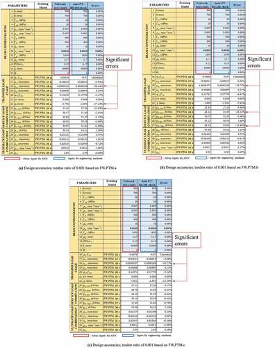
Figure 10. Design accuracies; tendon ratio of 0.002 based on PTM.

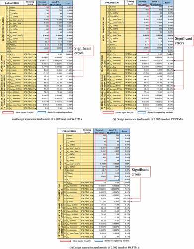
Table 4. Training summary based on PTM for a forward design.

(a) Training on Output 16–22
FORWARD PROBLEM:
15 Inputs ($b,h,fck,f_{cki},\rho st,\rho sc,f_{sy},f_{sw},{\varphi }_S,{\rho }_p,f_{py},{\varphi }_P,PTlos{s}_{lt},L,K_c$) – (7 + 6 + 5) Outputs:
(Transfer 7 Outputs: $\sigma c/fcki,\epsilon st,\epsilon sc,{\epsilon }_p,\sigma ct/fcki,cw,\mathrm{\Delta }$)
(Service Load 5 Outputs: $q_{L/250},q_{0.2mm},q_{0.6f_{ck}},q_{0.8f_{su}},q_{0.75f_{pu}}$)
(Ultimate Load 6 Outputs: $qstr,\epsilon st,\epsilon sc,\epsilon p,\rho sw,\mu \mathrm{\Delta }$)
No.			Data	Layers	Neurons	Validation check	Required Epoch	Best Epoch for Training	Stopped Epoch	Mean Square Error	R at Best Epoch	Comments
15 Inputs ($b,h,fck,f_{cki},\rho st,\rho sc,f_{sy},f_{sw},{\varphi }_S,{\rho }_p,f_{py},{\varphi }_P,PTlos{s}_{lt},L,K_c$) – 1 Output (Transfer$\sigma c/fcki$) – PTM
FW.PTM.	16	a	50,000	15	15	500	50,000	1,071	1,571	0.004782	0.944072	Insufficient
FW.PTM.	16	b	50,000	20	20	500	50,000	986	1,486	0.005467	0.940664	Insufficient
FW.PTM.	16	c	50,000	25	25	500	50,000	1,322	1,822	0.006158	0.937434	Insufficient
15 Inputs ($b,h,fck,f_{cki},\rho st,\rho sc,f_{sy},f_{sw},{\varphi }_S,{\rho }_p,f_{py},{\varphi }_P,PTlos{s}_{lt},L,K_c$) – 1 Output (Transfer$\epsilon st$) – PTM
FW.PTM.	17	a	50,000	15	15	500	50,000	8,397	8,897	3.18E-05	0.998924	Good
FW.PTM.	17	b	50,000	20	20	500	50,000	3,935	4,435	4.21E-05	0.998705	Good
FW.PTM.	17	c	50,000	25	25	500	50,000	12,330	12,830	3.90E-05	0.998705	Good
15 Inputs ($,h,fc,{ }_{cki},\rho st,\rho sc,f_{sy},f_{sw},{\varphi }_S,{\rho }_p,f_{py},{\varphi }_P,PTlos{s}_{lt},L,K_c$) – 1 Output (Transfer$\epsilon sc$) – PTM
FW.PTM.	18	a	50,000	15	15	500	50,000	3,708	4,208	9.75E-05	0.983229	Neutral
FW.PTM.	18	b	50,000	20	20	500	50,000	6,081	5,581	1.34E-04	0.979253	Neutral
FW.PTM.	18	c	50,000	25	25	500	50,000	4,425	4,925	1.32E-04	0.982499	Neutral
15 Inputs ($b,h,fck,f_{cki},\rho st,\rho sc,f_{sy},f_{sw},{\varphi }_S,{\rho }_p,f_{py},{\varphi }_P,PTlos{s}_{lt},L,K_c$) – 1 Output (Transfer$\epsilon p$) – PTM
FW.PTM.	19	a	50,000	15	15	500	50,000	7,784	8,284	2.78E-05	0.999136	Good
FW.PTM.	19	b	50,000	20	20	500	50,000	10,014	10,514	4.16E-05	0.998751	Good
FW.PTM.	19	c	50,000	25	25	500	50,000	15,211	15,711	2.38E-05	0.999307	Good
15 Inputs ($b,h,fck,f_{cki},\rho st,\rho sc,f_{sy},f_{sw},{\varphi }_S,{\rho }_p,f_{py},{\varphi }_P,PTlos{s}_{lt},L,K_c$) – 1 Output (Transfer$\sigma ct/fcki$) – PTM
FW.PTM.	20	a	50,000	15	15	500	50,000	5,531	6,031	4.75E-05	0.99888	Good
FW.PTM.	20	b	50,000	20	20	500	50,000	4,262	4,762	5.99E-05	0.998598	Good
FW.PTM.	20	c	50,000	25	25	500	50,000	14,267	14,767	5.57E-05	0.998716	Good
15 Inputs ($b,h,fck,f_{cki},\rho st,\rho sc,f_{sy},f_{sw},{\varphi }_S,{\rho }_p,f_{py},{\varphi }_P,PTlos{s}_{lt},L,K_c$) – 1 Output (Transfer$cw$) – PTM
FW.PTM.	21	a	50,000	15	15	500	50,000	1,690	2,190	8.41E-05	0.966521	Neutral
FW.PTM.	21	b	50,000	20	20	500	50,000	4,241	4,741	1.06E-04	0.958348	Neutral
FW.PTM.	21	c	50,000	25	25	500	50,000	8,261	8,761	9.61E-05	0.962456	Neutral
15 Inputs ($b,h,fck,f_{cki},\rho st,\rho sc,f_{sy},f_{sw},{\varphi }_S,{\rho }_p,f_{py},{\varphi }_P,PTlos{s}_{lt},L,K_c$) – 1 Output (Transfer$\mathrm{\Delta }$) – PTM
FW.PTM.	22	a	50,000	15	15	500	50,000	6,270	6,770	9.37E-06	0.998423	Good
FW.PTM.	22	b	50,000	20	20	500	50,000	3,303	3,803	2.97E-05	0.993811	Good
FW.PTM.	22	c	50,000	25	25	500	50,000	4,559	5,059	5.53E-05	0.992654	Good
(b) Training on Output 23–27
FORWARD PROBLEM:
15 Inputs ($b,h,fck,f_{cki},\rho st,\rho sc,f_{sy},f_{sw},{\varphi }_S,{\rho }_p,f_{py},{\varphi }_P,PTlos{s}_{lt},L,K_c$) – (7 + 6 + 5) Outputs:
(Transfer 7 Outputs: $\sigma c/fcki,\epsilon st,\epsilon sc,{\epsilon }_p,\sigma ct/fcki,cw,\mathrm{\Delta }$)
(Service Load 5 Outputs: $q_{L/250},q_{0.2mm},q_{0.6f_{ck}},q_{0.8f_{su}},q_{0.75f_{pu}}$)
(Ultimate Load 6 Outputs: $qstr,\epsilon st,\epsilon sc,\epsilon P,\rho sw,\mu \mathrm{\Delta }$)
No.			Data	Layers	Neurons	Validation check	Required Epoch	Best Epoch for Training	Stopped Epoch	Mean Square Error	R at Best Epoch	Comments
15 Inputs ($b,h,fck,f_{cki},\rho st,\rho sc,f_{sy},f_{sw},{\varphi }_S,{\rho }_p,f_{py},{\varphi }_P,PTlos{s}_{lt},L,K_c$) – 1 Output (Service$q_{L/250}$) – PTM
FW.PTM.	23	a	50,000	15	15	500	50,000	4,892	5,392	2.30E-05	0.998656	Good
FW.PTM.	23	b	50,000	20	20	500	50,000	10,102	10,602	2.61E-06	0.99986	Very good
FW.PTM.	23	c	50,000	25	25	500	50,000	14,343	14,843	2.32E-06	0.999879	Very good
15 Inputs ($b,h,fck,f_{cki},\rho st,\rho sc,f_{sy},f_{sw},{\varphi }_S,{\rho }_p,f_{py},{\varphi }_P,PTos{s}_{lt},L,K_c$) – 1 Output (Service$q_{0.2mm}$) – PTM
FW.PTM.	24	a	50,000	15	15	500	50,000	18,517	19,017	2.37E-07	0.999989	Very good
FW.PTM.	24	b	50,000	20	20	500	50,000	16,097	16,597	2.63E-06	0.999876	Very good
FW.PTM.	24	c	50,000	25	25	500	50,000	17,348	17,848	8.69E-07	0.999958	Very good
15 Inputs ($b,h,fck,f_{cki},\rho st,\rho sc,f_{sy},f_{sw},{\varphi }_S,{\rho }_p,f_{py},{\varphi }_P,PTlos{s}_{lt},L,K_c$) – 1 Output (Service$q_{0.6f_{ck}}$) – PTM
FW.PTM.	25	a	50,000	15	15	500	50,000	15,311	15,811	7.29E-07	0.999,962	Very good
FW.PTM.	25	b	50,000	20	20	500	50,000	15,522	16,022	7.52E-07	0.999962	Very good
FW.PTM.	25	c	50,000	25	25	500	50,000	18,775	19,275	9.69E-07	0.999954	Very good
15 Inputs ($b,h,fck,f_{cki},\rho st,\rho sc,f_{sy},f_{sw},{\varphi }_S,{\rho }_p,f_{py},{\varphi }_P,PTlos{s}_{lt},L,K_c$) – 1 Output (Service$q_{0.8f_{su}}$) – PTM
FW.PTM.	26	a	50,000	15	15	500	50,000	13,024	13,524	3.92E-06	0.999,809	Very good
FW.PTM.	26	b	50,000	20	20	500	50,000	5,021	5,521	2.11E-05	0.999004	Good
FW.PTM.	26	c	50,000	25	25	500	50,000	20,844	21,344	7.11E-06	0.999717	Very good
15 Inputs ($b,h,fck,f_{cki},\rho st,\rho sc,f_{sy},f_{sw},{\varphi }_S,{\rho }_p,f_{py},{\varphi }_P,PTlos{s}_{lt},L,K_c$) – 1 Output (Service$q_{0.75f_{pu}}$) – PTM
FW.PTM.	27	a	50,000	15	15	500	50,000	4,490	4,990	1.85E-05	0.999126	Good
FW.PTM.	27	b	50,000	20	20	500	50,000	9,634	10,134	5.49E-06	0.999703	Very good
FW.PTM.	27	c	50,000	25	25	500	50,000	6,148	6,648	2.24E-05	0.999177	Good
(c) Training on Output 28–33
FORWARD PROBLEM:
15 Inputs ($b,h,fck,f_{cki},\rho st,\rho sc,f_{sy},f_{sw},{\varphi }_S,{\rho }_p,f_{py},{\varphi }_P,PTlos{s}_{lt},L,K_c$) – (7 + 6 + 5) Outputs:
(Transfer 7 Outputs: $\sigma c/fcki,\epsilon st,\epsilon sc,{\epsilon }_p,\sigma ct/fcki,cw,\mathrm{\Delta }$)
(Service Load 5 Outputs: $q_{L/250},q_{0.2mm},q_{0.6f_{ck}},q_{0.8f_{su}},q_{0.75f_{pu}}$)
(Ultimate Load 6 Outputs: $qstr,\epsilon st,\epsilon sc,\epsilon P,\rho sw,\mu \mathrm{\Delta }$)
No.			Data	Layers	Neurons	Validation check	Required Epoch	Best Epoch for Training	Stopped Epoch	Mean Square Error	R at Best Epoch	Comments
15 Inputs ($b,h,fck,f_{cki},\rho st,\rho sc,f_{sy},f_{sw},{\varphi }_S,{\rho }_p,f_{py},{\varphi }_P,PTlos{s}_{lt},L,K_c$) – 1 Output (Ultimate$q_{str}$) – PTM
FW.PTM.	28	a	50,000	15	15	500	50,000	17,103	17,603	1.01E-05	0.99962	Good
FW.PTM.	28	b	50,000	20	20	500	50,000	8,466	8,966	1.36E-05	0.999481	Good
FW.PTM.	28	c	50,000	25	25	500	50,000	8,643	9,143	2.35E-05	0.99908	Good
15 Inputs ($b,h,fck,f_{cki},\rho st,\rho sc,f_{sy},f_{sw},{\varphi }_S,{\rho }_p,f_{py},{\varphi }_P,PTlos{s}_{lt},L,K_c$) – 1 Output (Ultimate$\epsilon st$) – PTM
FW.PTM.	29	a	50,000	15	15	500	50,000	2,002	2,502	1.19E-04	0.999265	Neutral
FW.PTM.	29	b	50,000	20	20	500	50,000	4,198	4,698	8.08E-05	0.999451	Good
FW.PTM.	29	c	50,000	25	25	500	50,000	11,860	12,360	2.60E-05	0.999857	Good
15 Inputs ($b,h,fck,f_{cki},\rho st,\rho sc,f_{sy},f_{sw},{\varphi }_S,{\rho }_p,f_{py},{\varphi }_P,PTlos{s}_{lt},L,K_c$) – 1 Output (Ultimate$\epsilon sc$) – PTM
FW.PTM.	30	a	50,000	15	15	500	50,000	5,690	6,190	1.00E-04	0.998833	Neutral
FW.PTM.	30	b	50,000	20	20	500	50,000	8,964	9,464	8.03E-05	0.999406	Good
FW.PTM.	30	c	50,000	25	25	500	50,000	10,401	10,901	4.00E-05	0.999559	Good
15 Inputs ($b,h,fck,f_{cki},\rho st,\rho sc,f_{sy},f_{sw},{\varphi }_S,{\rho }_p,f_{py},{\varphi }_P,PTlos{s}_{lt},L,K_c$) – 1 Output (Ultimate${\epsilon }_p\hspace{0.17em}$) – PTM
FW.PTM.	31	a	50,000	15	15	500	50,000	7,733	8,233	2.79E-05	0.99979	Good
FW.PTM.	31	b	50,000	20	20	500	50,000	5,486	5,986	4.92E-05	0.999644	Good
FW.PTM.	31	c	50,000	25	25	500	50,000	8,574	9,074	6.39E-05	0.999697	Good
15 Inputs ($b,h,fck,f_{cki},\rho st,\rho sc,f_{sy},f_{sw},{\varphi }_S,{\rho }_p,f_{py},{\varphi }_P,PTlos{s}_{lt},L,K_c$) – 1 Output (Ultimate$\rho sw$) – PTM
FW.PTM.	32	a	50,000	15	15	500	50,000	10,874	11,374	1.56E-05	0.999823	Good
FW.PTM.	32	b	50,000	20	20	500	50,000	12,317	12,817	1.76E-05	0.999865	Good
FW.PTM.	32	c	50,000	25	25	500	50,000	13,555	14,055	1.30E-05	0.999914	Good
15 Inputs ($b,h,fck,f_{cki},\rho st,\rho sc,f_{sy},f_{sw},{\varphi }_S,{\rho }_p,f_{py},{\varphi }_P,PTlos{s}_{lt},L,K_c$) – 1 Output (Ultimate${\mu }_{\mathrm{\Delta }}$) – PTM
FW.PTM.	33	a	50,000	15	15	500	50,000	6,413	6,913	6.33E-05	0.998257	Good
FW.PTM.	33	b	50,000	20	20	500	50,000	9,294	9,794	4.27E-05	0.998717	Good
FW.PTM.	33	c	50,000	25	25	500	50,000	7,693	8,193	7.33E-05	0.99824	Good
FW.PTM.16a

Note: Three PTMs for each output:• PTM a: 15 layers, 15 neurons, 500 validation checks• PTM a: 20 layers, 20 neurons, 500 validation checks• PTM a: 25 layers, 25 neurons, 500 validation checks

4.2. Design charts corresponding to ρ_p for forward design

Design charts shown in Figure 11 are established based on the following parameters; pre-assigned inputs are parameters b = 500 mm, h = 700 mm, f_ck = 40 MPa, f_cki = 20 MPa, ρ_st = 0.005, ρ_sc = 0.005, f_sy = 500 MPa, f_sw = 400 MPa, ${\varphi }_s$= 16 mm, f_py = 1650 MPa, ${\varphi }_p$= 12.7 mm, PTLoss_lt = 0.15, L = 10,000 mm, and K_c = 3; output parameter is σ_c/f_cki at transfer stage.

Figure 11. Design charts corresponding to ρ_p.

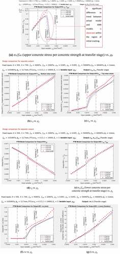
In Figure 11, design parameters (σ_c/f_cki,ε_st,ε_sc,ε_p, and σ_ct/f_cki) are plotted in Y-axis by varying tendon ratio (ρ_p) which is shown with X-axis. In Figure 11(a), σ_c/f_cki (Output # 16) represents upper concrete stress per concrete strength at transfer stage. Upper concrete is usually in tension during the transfer stage because the load is upward. In actual concrete sections, tension concrete stresses (${\sigma }_c$ of Output # 16 and ${\sigma }_{ct}$ Output # 20) immediately falls to 0 when reaching its tensile concrete strength at the transfer stage (f_cki) by an assumption that tensile concrete strength is lost after cracking. A discontinuity is shown in tensile concrete sections due to this assumption, whereas an ANN with a feed-forward network approximates a discontinuity based on real-valued continuous functions. A significant difference in data tendency between tensile concrete sections and ANNs is observed at the vicinity of initial cracking.

Figures 11(b-e) plotted based on Figures 9 and 10 present design aides for ε_st,ε_sc,ε_p, and σ_ct/f_cki (Output # 17, 18, 19, and 20, respectively) as a function of ρ_p. Design parameters (ε_st,ε_sc,ε_p, and σ_ct/f_cki) are obtained rapidly and accurately for a given tendon ratio (ρ_p). Figures 11(f-g) also show plots for cw (Output # 21) vs. ρ_p and Δ (Output # 22) vs. ρ_p, respectively.

5. Reverse design based on artificial neural networks (ANNs)

5.1. Design based on PTM using deep neural networks (DNN)

5.1.1. Formulation of ANNs based on back-substitution (BS) applicable to reverse designs

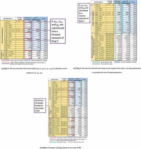
In a reverse scenario shown in Figure 8(b) and Table 5, design parameters (b, ρ_st,ρ_sc, and ρ_p in green cell) targeting nominal capacities (q_L/250,q_{0.2 mm},q_str, and μ_Δ in the yellow cell) are calculated on an output-side the reverse network of Step 1. Table 5 summarizes the training accuracy based on PTM. An ANN trained by R3.PTM.a based on 20 layers-20 neurons is used to calculate design parameters (b, ρ_st,ρ_sc, and ρ_p) as shown in Boxes 1, 5, 6, and 10 on an output-side the Step 1 of Figure 12.

Figure 12. Design results based on 20 layers-20 neurons for Step 1;q_L/250 = 80 kN/m at SLL (at a deflection of L/250), q_str = 150 kN/m at ULL, and deflection ductility ratios (μ_Δ) of 1.50 at ULL.

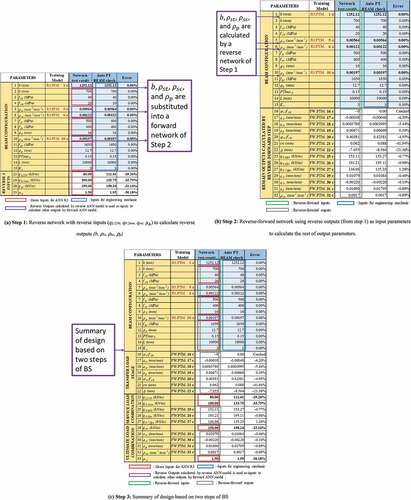
Table 5. Training accuracies of a reverse scenario based on PTM; reverse network of Step 1.

REVERSE NETWORK OF STEP 1-REVERSE SCENARIO 15 Inputs ($h,fck,f_{cki},f_{sy},f_{sw},{\varphi }_S,f_{py},{\varphi }_P,PTlos{s}_{lt},L,K_c,q_{L/250},q_{0.2mm},qstr,{\mu }_{\mathrm{\Delta }}$) – (4) Outputs ($b,\hspace{0.17em}\rho st,\rho sc,{\rho }_p)$
No.			Data	Layers	Neurons	Validation check	Required Epoch	Best Epoch for Training	Stopped Epoch	Mean Square Error	R at Best Epoch	Comments
15 Inputs ($h,fck,f_{cki},f_{sy},f_{sw},{\varphi }_S,f_{py},{\varphi }_P,PTlos{s}_{lt},L,K_c,q_{L/250},q_{0.2mm},qstr,{\mu }_{\mathrm{\Delta }}$) – 1 Output ($b$) – PTM
R3.PTM.	1	a	50,000	20	20	500	50,000	31,407	31,907	0.001083	0.990338	Neural
R3.PTM.	1	b	50,000	30	30	1000	70,000	67,507	68,507	0.000714	0.994255	Neural
R3.PTM.	1	c	50,000	40	40	5000	100,000	55,324	60,324	0.000764	0.994578	Neural
15 Inputs ($h,fck,f_{cki},f_{sy},f_{sw},{\varphi }_S,f_{py},{\varphi }_P,PTlos{s}_{lt},L,K_c,q_{L/250},q_{0.2mm},qstr,{\mu }_{\mathrm{\Delta }}$) – 1 Output ($\rho st$) – PTM
R3.PTM.	5	a	50,000	20	20	500	50,000	27,052	27,552	1.67E-03	0.989345	Insufficient
R3.PTM.	5	b	50,000	30	30	1000	70,000	47,114	48,114	0.001197	0.994218	Neural
R3.PTM.	5	c	50,000	40	40	5000	100,000	48,774	53,774	9.18E-04	0.995224	Neural
15 Inputs ($h,fck,f_{cki},f_{sy},f_{sw},{\varphi }_S,f_{py},{\varphi }_P,PTlos{s}_{lt},L,K_c,q_{L/250},q_{0.2mm},qstr,{\mu }_{\mathrm{\Delta }}$) – 1 Output ($\rho sc$) – PTM
R3.PTM.	6	a	50,000	20	20	500	50,000	18,532	19,032	1.45E-02	0.911693	Insufficient
R3.PTM.	6	b	50,000	30	30	1000	70,000	26,751	27,751	0.013178	0.929903	Insufficient
R3.PTM.	6	c	50,000	40	40	5000	100,000	35,302	40,302	1.29E-02	0.9375	Insufficient
15 Inputs ($h,fck,f_{cki},f_{sy},f_{sw},{\varphi }_S,f_{py},{\varphi }_P,PTlos{s}_{lt},L,K_c,q_{L/250},q_{0.2mm},qstr,{\mu }_{\mathrm{\Delta }}$) – 1 Output (${\rho }_p$) – PTM
R3.PTM.	10	a	50,000	20	20	500	50,000	18,887	19,387	7.82E-03	0.937977	Insufficient
R3.PTM.	10	b	50,000	30	30	1000	70,000	30,611	31,611	0.004052	0.976151	Neural
R3.PTM.	10	c	50,000	40	40	5000	100,000	37,338	42,338	3.41E-03	0.9796	Neural

An ANN with FW.PTM.c based on 40 layers and 40 neurons is implemented in training the forward network of Step 2, when 18 outputs including reverse input parameters (q_L/250,q_{0.2 mm},q_str, and μ_Δ which were already prescribed in Boxes 23, 24, 28, and 33 in Step 1) are calculated in Boxes 16 to 33 on an output-side of Step 2. Fifteen input design parameters including b, ρ_st,ρ_sc, and ρ_p pre-calculated on an output-side the reverse network of Step 1 are used in Boxes 1 to 15 of the forward network of Step 2.

5.1.2. Design accuracies

5.1.2.1. Adjusting reverse input parameters to enhance design accuracies

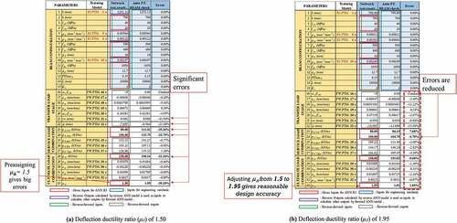
In Figure 12 of a reverse scenario, selected design parameters include input parameters as follows; h = 700 mm, f_ck = 40 MPa, f_cki = 20 MPa, f_sy = 500 MPa, f_sw = 400 MPa, ф_s = 16 mm, (diameter of rebar), f_py = 1650 MPa, ф_p = 12.7 mm (diameter of tendon), PTLoss_lt = 0.15, L = 10,000, and K_c = 3 when the following reverse parameters are reversely pre-assigned on an input-side; q_L/250 = 80 KN/m (SLL), q_{0.2 mm} = 100 KN/m (SLL), q_str = 150 KN/m (ULL), and deflection ductility ratios (μ_Δ) of 1.5.

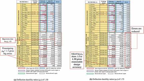
When a deflection ductility ratio (μ_Δ) of 1.50 is used, the reverse network of Step 1 produces a beam width (b) of 1252.12 mm, a lower tensile rebar ratio (ρ_st) of 0.00564, a compressive rebar ratio (ρ_sc) of 0.00122, and a tendon ratio (ρ_p) of 0.00197 in Boxes 1, 5, 6, and 10 on the output side of Figure 12(a). Significant errors are caused in a design as shown in Step 2 forward network, with the largest errors reaching −41.94% (0.062 mm vs. 0.088 mm) and −21.38% (−7.055 mm vs. −8.564 mm) for crack width and deflection (camber) at transfer load limit state, respectively, as shown in Figure 12(b). This is due to the reverse input parameter such as deflection ductility ratio (μ_Δ) of 1.50 being incorrectly pre-assigned out of data range at ULL in Step 1 of Figure 12. Errors of crack width and deflection (camber) at transfer load limit state reach −8.00% (0.050 mm vs. 0.054 mm) and 15.58% (−10.985 mm vs. −12.696 mm), respectively, indicating that errors decrease when deflection ductility ratio (μ_Δ) of 1.50 is adjusted to 1.95 as shown in Figure 13(b). These design parameters lead to targeted nominal capacities resisting applied distributed load (q_L/250 = 80 kN/m) shown in Box 23 of Figure 13(b) with an error equal to −7.68% (80 kN/m vs. 86.15 kN/m) when the deflection reaches L/250 at SLL. An error is −39.26% for q_L/250 when the deflection ductility ratio (μ_Δ) of 1.50 is used as shown in Box 28 of Figure 13(a). An error of −0.68% (150 kN/m vs. 151.02 kN/m) for nominal capacities of q_str = 150 kN/m shown in Box 28 of Figure 13(b) is also improved when compared to an error of −32.16% shown in Figure 13(a).

Figure 13. Design results based on 20 layers-20 neurons for Step 1; q_L/250 = 80 kN/m at SLL (at a deflection of L/250), q_str = 150 kN/m at ULL, and deflection ductility ratio (μ_Δ) of 1.50 adjusted to 1.95 at ULL.

5.1.2.2. Influence of layer and neurons on design accuracies

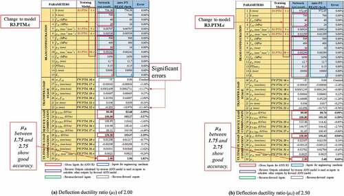
Figures 14-16 shows how a number of hidden layers and neurons influence the accuracies of reverse designs. ANNs based on R3.PTM.a, R3.PTM.b, and R3.PTM.c based on 20 layers-20 neurons, 30 layers-30 neurons, and 40 layers-40 neurons are implemented in the reverse network of Step 1 of Figures 14-16, respectively, where the deflection ductility ratio (μ_Δ) of 2.00 is adjusted to 2.50. An ANN with FW.PTM.c based on 40 layers and 40 neurons is trained in the forward network of Step 2 to obtain 18 outputs in Boxes 16 to 33. The best design accuracies are found with ANNs using R3.PTM.c, which is based on 40 layers-40 neurons and based on a deflection ductility ratio (μ_Δ) of 2.50. The network parameters depend on a number of hidden layers and neurons. Input conflicts should also be removed by selecting reversely pre-assigned input parameters that satisfy structural mechanics.

Figure 14. Design results based on 20 layers-20 neurons for Step 1; q_L/250 = 80 kN/m at SLL (at a deflection of L/250), q_str = 150 kN/m at ULL, and deflection ductility ratio (μ_Δ) of 2.00 and 2.50 at an ultimate load limit state (ULL).

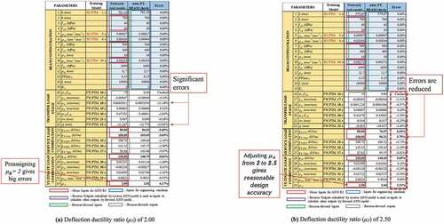
Figure 15. Design results 30 layers-30 neurons for Step 1 neurons for Step 1; q_L/250 = 80 kN/m at SLL (at a deflection of L/250), q_str = 150 kN/m at ULL, deflection ductility ratio (μ_Δ) of 2.00 and 2.50 at an ultimate load limit state (ULL).

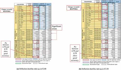
Figure 16. Design results 40 layers-40 neurons for Step 1 neurons for Step 1; q_L/250 = 80 kN/m at SLL (at a deflection of L/250), q_str = 150 kN/m at ULL, deflection ductility ratio (μ_Δ) of 2.00 and 2.50 at an ultimate load limit state (ULL).

5.2. Design based on CRS using deep neural networks (DNN)

5.2.1. Formulation of ANNs based on back-substitution (BS) applicable to reverse designs

Readers are referred to the book (Hong 2021) to review the CRS method which is used in training the reverse network. A sequence of training networks should be determined based on the feature scores shown in Table 6(a). Reverse inputs (q_L/250,q_{0.2 mm},q_str, and μ_Δ) are pre-assigned in the reverse network of Step 1 to calculate reverse outputs (b, ρ_st,ρ_sc, and ρ_p) as shown in Reverse Scenario 3 of Table 6(b), where training accuracies based on CRS with deep neural networks (DNN) are presented.

Table 6. Training sequence of a reverse scenario based on CRS (DNN).

(a) Feature scores based on NCA
(b) Training accuracies of a reverse Scenario based on CRS (DNN)
REVERSE NETWORK OF STEP 1-REVERSE SCENARIO
15 Inputs ($h,fck,f_{cki},f_{sy},f_{sw},{\varphi }_S,f_{py},{\varphi }_P,PTlos{s}_{lt},L,K_c,q_{L/250},q_{0.2mm},qstr,{\mu }_{\mathrm{\Delta }}$) – (4) Outputs ($b,\hspace{0.17em}\rho st,\rho sc,{\rho }_p)$
No.			Data	Layers	Neurons	Validation check	Required Epoch	Best Epoch for Training	Stopped Epoch	Mean Square Error	R at Best Epoch	Comments
15 Inputs ($h,fck,f_{cki},f_{sy},f_{sw},{\varphi }_S,f_{py},{\varphi }_P,PTlos{s}_{lt},L,K_c,q_{L/250},q_{0.2mm},qstr,{\mu }_{\mathrm{\Delta }}$) – 1 Output ($b$) – PTM
R3.PTM.	1	a	50,000	20	20	500	50,000	31,407	31,907	1.1E-03	1.1E-03	0.99034
R3.PTM.	1	b	50,000	30	30	1000	70,000	67,507	68,507	7.1E-04	7.3E-04	0.99425
R3.PTM.	1	c	50,000	40	40	5000	100,000	55,324	60,324	7.6E-04	7.5E-04	0.99458
16 Inputs ($h,fck,f_{cki},f_{sy},f_{sw},{\varphi }_S,f_{py},{\varphi }_P,PTlos{s}_{lt},L,K_c,q_{L/250},q_{0.2mm},qstr,{\mu }_{\mathrm{\Delta }},b$) – 1 Output ($\rho st$) – CRS
R3.CRS.	5	a	50,000	20	20	500	50,000	24,914	25,414	1.7.E-04	1.7.E-04	0.99908
R3.CRS.	5	b	50,000	30	30	1000	100,000	40,601	41,601	9.9.E-05	1.1.E-04	0.99947
R3.CRS.	5	c	50,000	40	40	5000	100,000	51,497	56,497	7.3.E-05	9.1.E-05	0.99969
17 Inputs ($h,fck,f_{cki},f_{sy},f_{sw},{\varphi }_S,f_{py},{\varphi }_P,PTlos{s}_{lt},L,K_c,q_{L/250},q_{0.2mm},qstr,{\mu }_{\mathrm{\Delta }},b,\rho st$) – 1 Output ($\rho sc$) – CRS
R3.CRS.	10	a	50,000	20	20	500	50,000	26,261	26,761	2.3.E-04	2.3.E-04	0.99835
R3.CRS.	10	b	50,000	30	30	1000	100,000	35,490	36,490	1.2.E-04	1.2.E-04	0.99919
R3.CRS.	10	c	50,000	40	40	5000	100,000	99,850	100,000	3.2.E-05	3.2.E-05	0.99982
18 Inputs ($h,fck,f_{cki},f_{sy},f_{sw},{\varphi }_S,f_{py},{\varphi }_P,PTlos{s}_{lt},L,K_c,q_{L/250},q_{0.2mm},qstr,{\mu }_{\mathrm{\Delta }},b,\rho st,,\rho sc$) – 1 Output ($\rho p$) – CRS
R3.CRS.	6	a	50,000	20	20	500	50,000	5,096	5,596	2.4.E-03	2.2.E-03	0.98852
R3.CRS.	6	b	50,000	30	30	1000	100,000	7,630	8,630	2.5.E-03	2.2.E-03	0.98743
R3.CRS.	6	c	50,000	40	40	5000	100,000	7,887	12,887	2.5.E-03	3.0.E-03	0.98848
Note: R3.CRS.10a

Training a reverse ANN in Step 1 using the CRS method, rather than the PTM described in Section 5.1, begins with beam width (b) because beam width (b) can be used to train networks without other output parameters, such as ρ_st,ρ_sc, and ρ_p, as feature indexes as shown in Table 6. Important feature indexes affecting beam width (b) include h (5.77), L (10.92), q_L/250 (4.14), q_{0.2 mm} (19.05), and q_str (3.04) without ρ_st and ρ_p as shown in Table 6. Numbers in Table 6(a) indicate feature scores selected using the NCA method (Hong and Pham 2021). As shown in Table 6(b), beam width (b) is, then, used as a feature index to train ρ_st, resulting in higher training accuracy for ρ_st. Similarly, beam width (b) and ρ_st are used as feature indexes to train ρ_p, followed by training ρ_sc using all output parameters, beam width (b), ρ_st, and ρ_p, as feature indexes. The output parameters located on an output-side cannot be used to train other output parameters when using the TED training method (Hong 2021).

5.2.2. Design accuracies

Lower rebar ratio (ρ_st) has a feature score of 18.70 on ρ_p whereas the upper rebar ratio (ρ_sc) is influenced by lower tensile rebar ratio (ρ_st) and tendon ratio (ρ_p) as much as 11.35 and 3.74, respectively. In the back-substitution method, ANNs with R3.CRS.aare trained based on 20 layers-20 neurons, respectively, for the reverse networks of Step 1 as shown in Figure 17 whereas an ANN with FW.PTM.c based on 40 layers and 40 neurons is implemented in training the forward network of Step 2 when 18 outputs including reverse input parameters (q_L/250,q_{0.2 mm},q_str, and μ_Δ which are already reversely prescribed in Boxes 23, 24, 28, and 33 in Step 1) are calculated in Boxes 16 to 33 as shown in Figure 17. It is noted that an ANN is trained on beam width b based on R3.PTM.b with 30 layers-30 neurons.

Figure 17. Design accuracies of a reverse scenario based on CRS (DNN); q_L/250 = 80 kN/m at SLL (at a deflection of L/250), q_str = 150 kN/m at ULL, deflection ductility ratio (μ_Δ) of 2.00 at ULL; 20 layers-20 neurons for Step 1.

In designs, q_L/250 = 80 kN/m at a deflection of L/250 at SLL and q_str = 150 kN/m at ULL are reversely pre-assigned on an input side. Design accuracies based on the reversely pre-assigned deflection ductility ratio (μ_Δ) of 2.00 shown in Figure 17(c) are acceptable. Design accuracies based on reversely pre-assigned deflection ductility ratios (μ_Δ) of 1.75 shown in Figures 18(b) are acceptable whereas those based on pre-assigned deflection ductility ratios (μ_Δ) of 1.50 shown in Figures 18(a) yield errors that are unacceptable for use in design practice. Input conflicts occur when the deflection ductility ratios (μ_Δ) is 1.5. Deflection ductility ratios (μ_Δ) are adjusted from 1.50 to 1.75 as shown in Figures 18(a,b) to be within large data ranges.

Figure 18. Design accuracies of a reverse scenario based on CRS (DNN); q_L/250 = 80 kN/m at SLL (at a deflection of L/250), q_str = 150 kN/m at ULL, deflection ductility ratio (μ_Δ) of 1.50 adjusted to 1.75 at ULL; 20 layers-20 neurons for Step 1.

Figures 19-21 investigates the influence of a number of layers-neurons used for CRS in Step 1 on design accuracies of ANNs for a reverse design. For the reverse networks of Step 1, ANNs with R3.CRS.a, R3.CRS.b, and R3.CRS.c are trained using 20 layers-20 neurons, 30 layers-30 neurons, and 40 layers-40 neurons, respectively, as shown in Figures 19-21 for reversely pre-assigned deflection ductility ratios (μ_Δ) of 2.00 and 2.50. When FW.PTM.c based on R3.CRS.a, R3.CRS.b, and R3.CRS.c is used, design accuracies similar to those of the three networks are found. For the reverse network of Step 1 trained based on 40 layers-40 neurons shown in Figure 21(b), the largest error is found with −9.32% (91.98 kN/m vs.100.56 kN/m when compared to those calculated based on structural mechanics) for q_0.75fpu that represents nominal strength when tendons reach stresses smaller of 0.75 f_pu and f_py. The next largest error of deflection (camber) at transfer load limit state reaches −7.27% (−9.896 mm vs. −10.616 mm) compared with those calculated using structural mechanics. Good accuracies among all three designs shown in Figures 19-21 are obtained when deflection ductility ratios (μ_Δ) within a range between 1.75 and 2.75 are trained. Fewer input conflicts occur with a deflection ductility ratio (μ_Δ) of 2.50 than with 2.00.

Figure 19. Design accuracies of a reverse scenario based on CRS (DNN); q_L/250 = 80 kN/m at a deflection of L/250 at SLL, q_str = 150 kN/m at ULL, and deflection ductility ratios (μ_Δ) of 2.00, 2.50 at ULL; 20 layers-20 neurons for Step 1.

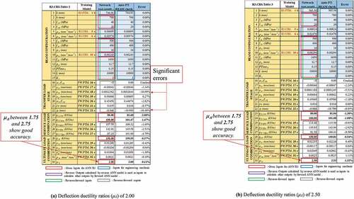
Figure 20. Design accuracies of a reverse scenario based on CRS (DNN); q_L/250 = 80 kN/m at a deflection of L/250 at SLL, q_str = 150 kN/m at ULL, and deflection ductility ratios (μ_Δ) of 2.00, 2.50 at ULL; 30 layers-30 neurons for Step 1.

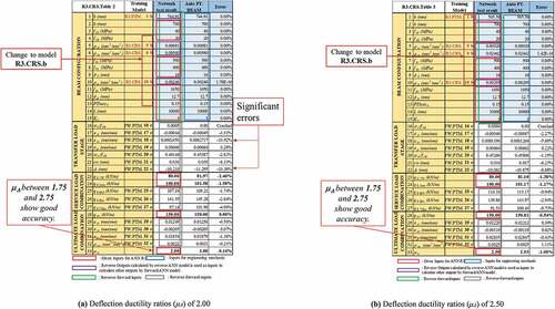
Figure 21. Design accuracies of a reverse scenario based on CRS (DNN); q_L/250, 80 kN/m at a deflection of L/250 at SLL, q_str 150 kN/m at ULL, and deflection ductility ratios (μ_Δ) of 2.00, 2.50 at ULL; 40 layers-40 neurons for Step 1.

It should be noted that networks used in the first reverse networks of Step 1 can be replaced by CRS to improve design accuracy.

5.2.3. Over-fitting

Because over-fitting occurs during training ANNs, the design accuracies are obtained using R3.CRS.c (40 layers-40 neurons) in Figure 21 are slightly lower than those obtained using R3.CRS.a (20 layers-20 neurons) and R3.CRS.b (30 layers-30 neurons) in Figures 19 and 20. When 20 layers-20 neurons are used, design accuracies comparable to those obtained with 30 layers-30 neurons are obtained.

5.2.4. Design charts

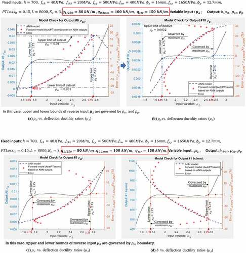
Figures 22(a-d) present reciprocal design charts for design parameters of ρ_sc,ρ_p,ρ_st, and b concerning ductility (μ_Δ). Design parameters of ρ_sc,ρ_p,ρ_st, and b are determined accurately based on deflection ductility ratios (μ_Δ) within ranges between 1.75 and 2.75 as shown in Figures 22(a-d), indicating that upper and lower bounds of deflection ductility ratios (μ_Δ) are governed by of ρ_sc,ρ_p,ρ_st, and b as can be seen in Figure 22. Design charts to determine ρ_sc,ρ_p,ρ_st, and b are obtained using Figures 14-21 obtained based on the boundary of deflection ductility ratios (μ_Δ) between 1.75 and 2.75. Errors increase rapidly outside this region in which AutoPTbeam results also diverge. Figures 22(a-d) are useful for calculating design parameters, ρ_sc,ρ_p,ρ_st, and b, for specified deflection ductility ratios (μ_Δ) between 1.75 and 2.75.

Figure 22. Reciprocal design charts, errors indicated.

5.2.5. Design examples

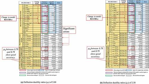
Figures 23-27 show additional design examples for a reverse scenario based on CRS (DNN) that investigate the influence of a number of layers-neurons for Step 1 on design accuracies. In Figures 23 and 24, ANNs with R3.CRS.b and R3.CRS.c are trained using 30 layers-30 neurons and 40 layers-40 neurons, respectively, for the reverse networks of Step 1 when the deflection ductility ratios (μ_Δ) of 2.75 and 1.50 at ULL are reversely pre-assigned based on q_L/250 = 80 kN/m at SLL and q_str = 150 kN/m at ULL. ANNs with FW.PTM.c based on 40 layers and 40 neurons are used to train the forward network of Step 2, when 18 outputs including reverse input parameters (q_L/250,q_{0.2 mm},q_str, and μ_Δ which are already reversely prescribed in Boxes 23, 24, 28, and 33 in Step 1) are calculated in Boxes 16 to 33 as shown in Figures 23 and 24. However, design accuracies are not acceptable because the pre-assigned deflection ductility ratios (μ_Δ) are not with the range between 1.75 and 2.75 as shown in Figure 22.

Figure 23. Design accuracies of Reverse Scenario based on CRS (DNN); qL/250 = 80 kN/m at a deflection of L/250 at SLL, qstr = 150 kN/m at ULL, and deflection ductility ratios (μΔ) of 2.75, 1.50 at ULL; 30 layers-30 neurons for Step 1.

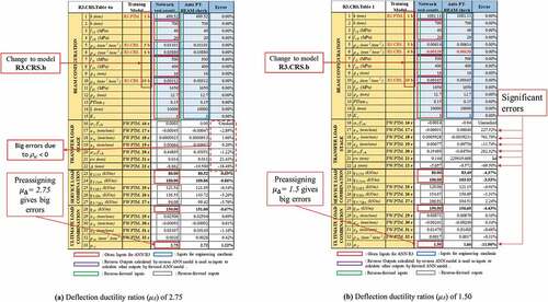
Figure 24. Design accuracies of Reverse Scenario based on CRS (DNN); q_L/250 = 80 kN/m at a deflection of L/250 at SLL, q_str = 150 kN/m at ULL, and deflection ductility ratios (μ_Δ) of 2.75, 1.50 at ULL; 40 layers-40 neurons for Step 1.

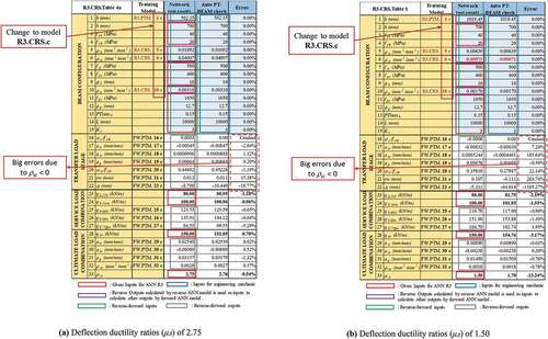
Figure 25. Design accuracies of Reverse Scenario based on CRS (DNN); q_L/250 = 80 kN/m at a deflection of L/250 at SLL, q_str = 150 kN/m at ULL, and deflection ductility ratios (μ_Δ) of 2.50, 3.00 at ULL; 30 layers-30 neurons for Step 1.

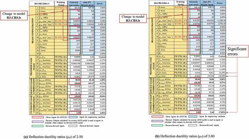
Figure 26. Design accuracies of Reverse Scenario based on CRS (DNN); q_L/250 = 80 kN/m at a deflection of L/250 at SLL, q_str = 150 kN/m at ULL, and deflection ductility ratios (μ_Δ) of 2.50, 3.00 at ULL; 40 layers-40 neurons for Step 1.

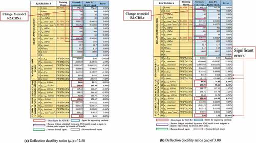
Figure 27. Design accuracies of Reverse Scenario based on CRS (DNN); q_L/250 = 80 kN/m at a deflection of L/250 at SLL, q_str = 150 kN/m at ULL, and deflection ductility ratios (μ_Δ) of 1.75, 2.00 at ULL; 40 layers-40 neurons and 30 layers-30 neurons for Step 1.

In Figures 25 and 26, ANNs with R3.CRS.b and R3.CRS.c are trained using 30 layers-30 neurons and 40 layers-40 neurons, respectively, for the reverse networks of Step 1 when deflection ductility ratios (μ_Δ) of 2.50 and 3.00 at ULL are reversely pre-assigned based on q_L/250 = 80 kN/m at SLL and q_str = 150 kN/m at ULL. ANNs with FW.PTM.c based on 40 layers and 40 neurons are used to train the forward network of Step 2, when 18 outputs including reverse input parameters (q_L/250,q_{0.2 mm},q_str, and μ_Δ which are already reversely prescribed in Boxes 23, 24, 28, and 33 in Step 1) are calculated in Boxes 16 to 33 as shown in Figures 25 and 26. Design accuracies based on the pre-assigned deflection ductility ratio (μ_Δ) of 2.50 are improved because the pre-assigned deflection ductility ratio (μ_Δ) is within the range between 1.75 and 2.75 whereas design accuracies based on the pre-assigned deflection ductility ratio (μ_Δ) of 3.00 are not improved as much as those with deflection ductility ratio (μ_Δ) of 2.50. After all, the ductility ratio (μ_Δ) of 3.00 falls outside the range between 1.75 and 2.75 as shown in Figure 22.

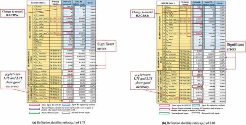
In Figures 27(a,b), ANNs with R3.CRS.c and R3.CRS.b are trained based on 40 layers-40 neurons and 30 layers-30 neurons for the reverse networks of Step 1, respectively. The deflection ductility ratios (μ_Δ) of 1.75 at ULL for Figure 27(a) and 2.00 at ULL and for Figure 27(b) are reversely pre-assigned based on q_L/250 = 80 kN/m at SLL and q_str = 150 kN/m at ULL. ANNs with FW.PTM.c based on 40 layers and 40 neurons are implemented in training the forward network of Step 2 when 18 outputs including reverse input parameters (q_L/250,q_{0.2 mm},q_str, and μ_Δ which are already reversely prescribed in Boxes 23, 24, 28, and 33 in Step 1) are calculated in Boxes 16 to 33 as shown in Figures 27(a,b). Design accuracies based on the pre-assigned deflection ductility ratio (μ_Δ) of 2.00 shown in Figures 27(b) are improved because the ductility ratio (μ_Δ) of 2.00 is within the range between 1.75 and 2.75 whereas design accuracies based on the ductility ratio (μ_Δ) of 1.75 shown in Figures 27(a) are not improved as much as those with the ductility ratio (μ_Δ) of 2.00. This is due to the ductility ratio (μ_Δ) of 1.75 being on the data region’s boundary, as shown in Figure 22.

5.3. Design based on CRS using shallow neural networks (SNN)

Table 7 presents training accuracies of a reverse scenario based on CRS using three types of deep and six types of shallow layers implemented in obtaining reverse outputs (b, ρ_st,ρ_sc, and ρ_p) in the reverse networks (based on DNN and SNN) of Step 1. The sequence of the training networks determined for deep layers is also used for shallow networks as can be seen in Table 7. The reverse output parameter, beam width b, is firstly obtained in Box 1 of Figure 28(a) based on R3.CRS.d. The rest of the reverse output parameters, ρ_st,ρ_sc, and ρ_p, based on R3.CRS.d are also obtained in Boxes 5, 6, and 10 of Figure 28(a), respectively. R3.CRS.a to R3.CRS.i using three types of deep and six types of shallow layers shown in Table 7 are tested to determine R3.CRS.d which produced the best design accuracies for b, ρ_st,ρ_sc, and ρ_p. Deep ANNs trained by R3.PTM.a to R3.PTM.c are used to map input parameters to beam width b based on 20 to 40 two hidden layers with 20 to 40 neurons and shallow ANNs trained by R3.PTM.d to R3.PTM.i based on one and two hidden layers with 20 to 40 neurons.

Table 7. Training accuracies of a reverse scenario based on deep and shallow ANNs; training accuracies obtained by mapping b based on PTM and ρ_st,ρ_sc, and ρ_p based on CRS.

REVERSE NETWORK OF STEP 1-REVERSE SCENARIO 3 15 Inputs ($h,fck,f_{cki},f_{sy},f_{sw},{\varphi }_S,f_{py},{\varphi }_P,PTlos{s}_{lt},L,K_c,q_{L/250},q_{0.2mm},qstr,{\mu }_{\mathrm{\Delta }}$) – (4) Outputs ($b,\hspace{0.17em}\rho st,\rho sc,{\rho }_p)$
No.			Data	Layers	Neurons	Validation check	Required Epoch	Best Epoch for Training	Stopped Epoch	Mean Square Error	R at Best Epoch	Comments
15 Inputs ($h,fck,f_{cki},f_{sy},f_{sw},{\varphi }_S,f_{py},{\varphi }_P,PTlos{s}_{lt},L,K_c,q_{L/250},q_{0.2mm},qstr,{\mu }_{\mathrm{\Delta }}$) – 1 Output ($b$) – PTM
R3.PTM.	1	a	50,000	20	20	500	50,000	31,407	31,907	1.1E-03	1.1E-03	0.99034
R3.PTM.	1	b	50,000	30	30	1000	70,000	67,507	68,507	7.1E-04	7.3E-04	0.99425
R3.PTM.	1	c	50,000	40	40	5000	100,000	55,324	60,324	7.6E-04	7.5E-04	0.99458
R3.PTM.	1	d	50,000	1	20	500	100,000	23,555	24,055	3.2E-03	3.3E-03	0.96889
R3.PTM.	1	e	50,000	1	30	500	100,000	27,598	28,098	2.8E-03	2.8E-03	0.97271
R3.PTM.	1	f	50,000	1	40	500	100,000	34,205	34,705	2.8E-03	2.7E-03	0.9747
R3.PTM.	1	g	50,000	2	20	500	100,000	55,209	55,709	1.2E-03	1.2E-03	0.98866
R3.PTM.	1	h	50,000	2	30	500	100,000	23,228	23,728	1.2E-03	1.1E-03	0.98954
R3.PTM.	1	i	50,000	2	40	500	100,000	31,943	32,443	1.1E-03	1.2E-03	0.99055
16 Inputs ($h,fck,f_{cki},f_{sy},f_{sw},{\varphi }_S,f_{py},{\varphi }_P,PTlos{s}_{lt},L,K_c,q_{L/250},q_{0.2mm},qstr,{\mu }_{\mathrm{\Delta }},b$) – 1 Output ($\rho st$) – CRS
R3.CRS.	5	a	50,000	20	20	500	50,000	24,914	25,414	1.7.E-04	1.7.E-04	0.99908
R3.CRS.	5	b	50,000	30	30	1000	100,000	40,601	41,601	9.9.E-05	1.1.E-04	0.99947
R3.CRS.	5	c	50,000	40	40	5000	100,000	51,497	56,497	7.3.E-05	9.1.E-05	0.99969
R3.CRS.	5	d	50,000	1	20	500	100,000	50,946	51,446	4.1.E-04	3.9.E-04	0.99756
R3.CRS.	5	e	50,000	1	30	500	100,000	36,977	37,477	3.3.E-04	3.3.E-04	0.99809
R3.CRS.	5	f	50,000	1	40	500	100,000	26,860	27,360	2.9.E-04	3.0.E-04	0.99824
R3.CRS.	5	g	50,000	2	20	500	100,000	29,700	30,200	2.2.E-04	2.2.E-04	0.99875
R3.CRS.	5	h	50,000	2	30	500	100,000	14,328	14,828	1.9.E-04	1.9.E-04	0.99891
R3.CRS.	5	i	50,000	2	40	500	100,000	6,637	7,137	2.6.E-04	2.7.E-04	0.99855
17 Inputs ($h,fck,f_{cki},f_{sy},f_{sw},{\varphi }_S,f_{py},{\varphi }_P,PTlos{s}_{lt},L,K_c,q_{L/250},q_{0.2mm},qstr,{\mu }_{\mathrm{\Delta }},b,\rho st$) – 1 Output ($\rho sc$) – CRS
R3.CRS.	10	a	50,000	20	20	500	50,000	26,261	26,761	2.3.E-04	2.3.E-04	0.99835
R3.CRS.	10	b	50,000	30	30	1000	100,000	35,490	36,490	1.2.E-04	1.2.E-04	0.99919
R3.CRS.	10	c	50,000	40	40	5000	100,000	99,850	100,000	3.2.E-05	3.2.E-05	0.99982
R3.CRS.	10	d	50,000	1	20	500	100,000	43,054	43,554	3.1.E-04	3.3.E-04	0.99776
R3.CRS.	10	e	50,000	1	30	500	100,000	28,699	29,199	2.7.E-04	2.8.E-04	0.99806
R3.CRS.	10	f	50,000	1	40	500	100,000	54,119	54,619	1.4.E-04	1.5.E-04	0.99902
R3.CRS.	10	g	50,000	2	20	500	100,000	42,064	42,564	1.4.E-04	1.5.E-04	0.99901
R3.CRS.	10	h	50,000	2	30	500	100,000	21,752	22,252	1.1.E-04	1.3.E-04	0.99921
R3.CRS.	10	i	50,000	2	40	500	100,000	42,061	42,561	4.1.E-05	4.8.E-05	0.99972
18 Inputs ($h,fck,f_{cki},f_{sy},f_{sw},{\varphi }_S,f_{py},{\varphi }_P,PTlos{s}_{lt},L,K_c,q_{L/250},q_{0.2mm},qstr,{\mu }_{\mathrm{\Delta }},b,\rho st,,\rho sc$) – 1 Output ($\rho p$) – CRS
R3.CRS.	6	a	50,000	20	20	500	50,000	5,096	5,596	2.4.E-03	2.2.E-03	0.98852
R3.CRS.	6	b	50,000	30	30	1000	100,000	7,630	8,630	2.5.E-03	2.2.E-03	0.98743
R3.CRS.	6	c	50,000	40	40	5000	100,000	7,887	12,887	2.5.E-03	3.0.E-03	0.98848
R3.CRS.	6	d	50,000	1	20	500	50,000	14,455	14,955	3.1.E-03	3.0.E-03	0.982
R3.CRS.	6	e	50,000	1	30	500	100,000	58,525	59,025	1.3.E-03	1.5.E-03	0.99171
R3.CRS.	6	f	50,000	1	40	500	100,000	23,233	23,733	1.2.E-03	1.4.E-03	0.99306
R3.CRS.	6	g	50,000	2	20	500	50,000	2,527	3,027	2.7.E-03	2.8.E-03	0.98471
R3.CRS.	6	h	50,000	2	30	500	100,000	12,373	12,873	1.1.E-03	1.2.E-03	0.99442
R3.CRS.	6	i	50,000	2	40	500	100,000	3,959	4,459	2.5.E-03	2.5.E-03	0.99007

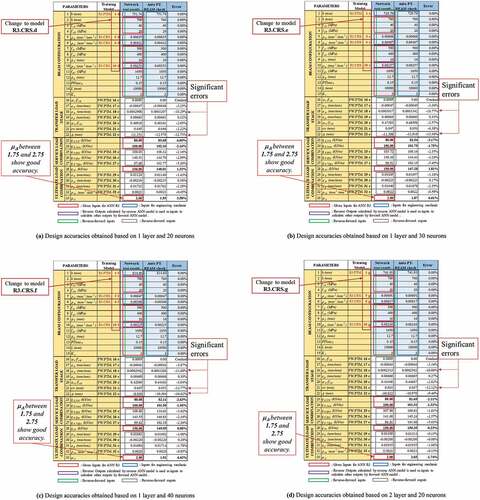
Figure 28. Design accuracies of Reverse Scenario 3 based on deep and shallow ANNs.

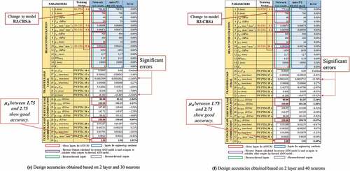
Similarly, deep ANNs trained by R3.CRS.a to R3.CRS.c based on 20 to 40 hidden layers – 20 to 40 neurons and shallow ANNs trained by R3.CRS.d to R3.CRS.i based on 1 and 2 hidden layers – 20 to 40 neurons are used to map input parameters to the rest of the reverse output parameters, ρ_st,ρ_sc, and ρ_p, respectively, For example, R3.CRS.10e represents an ANN trained based on 1 hidden layer – 30 neurons to obtain ρ_p in the reverse network of Step 1 as shown in Table 7. ANNs with FW.CRS.c are implemented in determining 18 outputs in the forward network of Step 2 as shown in Boxes 16 to 33 of Figure 28.

A dataset representing 15% of the total large datasets that are not used to train networks is used to verify training accuracies. Users can, however, provide the dataset ratio for verifying training accuracies. Figures 28(a-f) investigate the impact of a number of hidden layers and neurons implemented in Step 1 reverse networks on design accuracies obtained in Step 2 forward networks. When using shallow ANNs trained by R3.CRS.d to R3.CRS.i, design accuracies are similar to those obtained by deep ANNs trained by R3.CRS.a to R3.CRS.c, implying that ANNs trained with the CRS method in the reverse forward network of Step 1 can serve to determine accurate reverse outputs (b, ρ_st,ρ_sc, and ρ_p) with both deep and shallow layers as long as enough neurons are used. However, design accuracies heavily depend on the ranges of datasets. Pre-assigning a deflection ductility ratio (μ_Δ) out of the ranges between 1.7 to 2.75 causes significant errors as shown in Figure 28. The reversely pre-assigned input parameters should be adjusted to reduce design accuracies within the ranges between 1.7 to 2.75.

In Figure 28, design accuracies are compared with those based on structural calculations. Acceptable design accuracies are found as shown in Figures 28(a-f) where the a deflection ductility ratio (μ_Δ) of 2.00 is reversely pre-assigned on an input side. Errors of upper rebar strains (ε_sc) and deflection (camber) at transfer load limit state range from −10.77% to −11.68% and from −9.46% to −16.62%, respectively, when a reverse scenario is designed based on ANNs trained by R3.PTM.d, R3.CRS.e, R3.CRS.f, R3.CRS.g, R3.CRS.h, R3.CRS.i with 1 layer – 20 neurons as shown in Figures 28(a-f), respectively, where the deflection ductility ratios (μ_Δ) of 2.00.

5.4. Comparison of design based on CRS with those based on PTM

Figure 27(b) based on deep neural networks trained by R3.CRS.b (30 layers-30 neurons for the reverse network of Step 1) shows higher design accuracies compared with those obtained in Figure 16(a) based on ANNs trained by R3.PTM.c (40 layers-40 neurons) and Figure 28(e) based on shallow neural networks trained by R3.CRS.h (2 layers-30 neurons) when the deflection ductility ratios (μ_Δ) of 2.00 is reversely pre-assigned on an input-side.

6. Conclusions

Based on ANNs, this study demonstrates how to design pre-tensioned concrete beams. To establish reverse design scenarios, large amounts of input and output parameters are generated. For engineers, reverse designs with 15 input and 18 output parameters are proposed using ANN-trained reverse-forward networks. Here are some of the study’s findings.

(1) Two-step networks are formulated to solve reverse design scenarios. In the reverse network of Step 1, reverse output parameters are determined which are, then, used as input parameters in the forward network of Step 2 to determine the design parameters.

(2) TED, PTM, and CRS can be used for both the reverse and forward networks with selected training parameters such as a number of hidden layers, neurons, and validation checks. Extra input features can be selected from the output-side when training ANNs based on CRS which is not possible with TED, in which all inputs are mapped to entire outputs simultaneously. For additional explanations of training methods such as CRS and TED, readers are referred to the book (Hong 2021) and (Hong 2019).

(3) Selection of training networks depends on many parameters such as feature scores, the volume of datasets, and types of big datasets. In particular, when the volume of datasets is insufficient, deep neural networks (DNN) provide less accurate design accuracies than shallow neural networks (SNN). Deep neural networks trained with CRS outperform shallow neural networks trained with CRS and ANNs trained with PTM for the reverse network in Step 1.

(4) ANNs formulated to train reverses datasets generated from pre-tensioned concrete beams are adequate to produce acceptable design accuracies for use in practical designs. Design tables derived from reverse designs can be extended to plot design charts that connect all design parameters to achieve entire designs in a streak. The reverse design facilitates the rapid identification of design parameters, helping engineers with fast decisions based on acceptable accuracies.

Acknowledgments

This work was supported by the National Research Foundation of Korea (NRF) grant funded by the Korean government (MSIT 2019R1A2C2004965).

Disclosure statement

No potential conflict of interest was reported by the author(s).

Additional information

Funding

This work was supported by the National Research Foundation of Korea (NRF) grant funded by the Korean government [MSIT 2019R1A2C2004965].

Notes on contributors

Won-Kee Hong

Dr. Won-Kee Hong is a Professor of Architectural Engineering at Kyung Hee University. Dr. Hong received his Master’s and Ph.D. degrees from UCLA, and he worked for Englelkirk and Hart, Inc. (USA), Nihhon Sekkei (Japan) and Samsung Engineering and Construction Company (Korea) before joining Kyung Hee University (Korea). He also has professional engineering licenses from both Korea and the USA. Dr. Hong has more than 30 years of professional experience in structural engineering. His research interests include a new approach to construction technologies based on value engineering with hybrid composite structures. He has provided many useful solutions to issues in current structural design and construction technologies as a result of his research that combines structural engineering with construction technologies. He is the author of numerous papers and patents both in Korea and the USA. Currently, Dr. Hong is developing new connections that can be used with various types of frames including hybrid steel–concrete precast composite frames, precast frames and steel frames. These connections would help enable the modular construction of heavy plant structures and buildings. He recently published a book titled as “Hybrid Composite Precast Systems: Numerical Investigation to Construction” (Elsevier).

Manh Cuong Nguyen

Manh Cuong Nguyen is currently enrolled as a master candidate in the Department of Architectural Engineering at Kyung Hee University, Republic of Korea. His research interest includes AI and precast structures.

Tien Dat Pham

Tien Dat Pham is currently enrolled as a Ph.D. candidate in the Department of Architectural Engineering at Kyung Hee University, Republic of Korea. His research interest includes AI and precast structures.

Thuc Anh Le

Thuc Anh Le is currently enrolled as a master candidate in the Department of Architectural Engineering at Kyung Hee University, Republic of Korea. Her research interest includes AI and precast structures.

References

- Alhassan, M. A., A. N. Ababneh, and N. A. Betoush. 2020. “Innovative Model for Accurate Prediction of the Transfer Length of Prestressing Strands Based on Artificial Neural Networks: Case Study.” Case Studies in Construction Materials 12: e00312. doi:10.1016/j.cscm.2019.e00312.
- CEN (European Committee for Standardization). (2004). “Eurocode 2 : Part 1-1: General Rules and Rules for Buildings.” In Eurocode 2: Vol. BS En 1992.
- Hong, W. K. 2019. Hybrid Composite Precast Systems: Numerical Investigation to Construction. Elsevier: Woodhead Publishing.
- Hong, W. K. 2021.Artificial intelligence-based Design of Reinforced Concrete Structures.Daega.
- Hong, W. K., and M. C. Nguyen. 2021. “AI-based Lagrange Optimization for Designing Reinforced Concrete Columns.” Journal of Asian Architecture and Building Engineering 1–15. doi:10.1080/13467581.2021.1971998.
- Hong, W. K., V. T. Nguyen, and M. C. Nguyen. 2021. “Artificial intelligence-based Noble Design Charts for Doubly Reinforced Concrete Beams.” Journal of Asian Architecture and Building Engineering 1–23. doi:10.1080/13467581.2021.1928511.
- Hong, W.-K., M. C. Nguyen, and T. D. Pham. 2022. “Optimized Interaction P-M Diagram for Rectangular Reinforced Concrete Column Based on Artificial Neural Networks Abstract.” Journal of Asian Architecture and Building Engineering. doi:10.1080/13467581.2021.2018697.
- Hong, W. K., and T. D. Pham. 2021. “Reverse Designs of Doubly Reinforced Concrete Beams Using Gaussian Process Regression Models Enhanced by Sequence training/designing Technique Based on Feature Selection Algorithms.” Journal of Asian Architecture and Building Engineering 1–26. doi:10.1080/13467581.2021.1971999.
- Hong, W. K., T. D. Pham, and V. T. Nguyen. 2021. “Feature Selection Based Reverse Design of Doubly Reinforced Concrete Beams.” Journal of Asian Architecture and Building Engineering 1–25. doi:10.1080/13467581.2021.1928510.
- Khandel, O., M. Soliman, R. W. Floyd, and C. D. Murray. 2021. “Performance Assessment of Prestressed Concrete Bridge Girders Using Fiber Optic Sensors and Artificial Neural Networks.” Structure and Infrastructure Engineering 17 (5): 605–619. doi:10.1080/15732479.2020.1759658.
- Lee, K., S. Jeong, S. H. Sim, and D. H. Shin. 2019. “A Novelty Detection Approach for Tendons of Prestressed Concrete Bridges Based on A Convolutional Autoencoder and Acceleration Data.” Sensors (Switzerland) 19 (7). doi:10.3390/s19071633.
- MathWorks, (2022a). Deep Learning Toolbox: User's Guide (R2022a). Retrieved July 26, 20122 from: https://www.mathworks.com/help/pdf_doc/deeplearning/nnet_ug.pdf
- MathWorks, (2022b). Parallel Computing Toolbox: Documentation (R2022a). Retrieved July 26, from: https://uk.mathworks.com/help/parallel-computing/
- MathWorks, (2022c). Statistics and Machine Learning Toolbox: Documentation (R2022a). Retrieved July 26, from: https://uk.mathworks.com/help/stats/
- MathWorks, (2022d). MATLAB (R2022a)
- Mo, Y. L., and R. H. Han. 1995. “Investigation of Prestressed Concrete Frame Behavior with Neural Networks.” Journal of Intelligent Material Systems and Structures 6 (4): 566–573. doi:10.1177/1045389X9500600414.
- Naser, M. Z., and A. Alavi. 2020. “Insights into Performance Fitness and Error Metrics for Machine Learning.” arXiv Preprint arXiv 2006: 00887.
- Nguyen, M. C., and W. K. Hong. 2021. “Analytical Prediction of Nonlinear Behaviors of Beams post-tensioned by Unbonded Tendons considering Shear Deformation and Tension Stiffening Effect.” Journal of Asian Architecture and Building Engineering 1–22. doi:10.1080/13467581.2021.1908299.
- Slowik, O., D. Lehký, and D. Novák. 2021. “Reliability-based Optimization of a Prestressed Concrete Roof Girder Using a Surrogate Model and the double-loop Approach.” Structural Concrete 22 (4): 2184–2201. doi:10.1002/suco.202000455.
- Solhmirzaei, R., H. Salehi, V. Kodur, and M. Z. Naser. 2020. “Machine Learning Framework for Predicting Failure Mode and Shear Capacity of Ultra High Performance Concrete Beams.” Engineering Structures 224 (August): 111221. doi:10.1016/j.engstruct.2020.111221.
- Sumangala, K., and C. Antony Jeyasehar. 2011. “A New Procedure for Damage Assessment of Prestressed Concrete Beams Using Artificial Neural Network.” Advances in Artificial Neural Systems 2011: 1–9. doi:10.1155/2011/786535.
- Tam, C. M., T. K. L. Tong, T. C. T. Lau, and K. K. Chan. 2004. “Diagnosis of Prestressed Concrete Pile Defects Using Probabilistic Neural Networks.” Engineering Structures 26 (8): 1155–1162. doi:10.1016/j.engstruct.2004.03.018.
- Torky, A. A., and A. A. Aburawwash. 2018. “A Deep Learning Approach to Automated Structural Engineering of Prestressed Members.” International Journal of Structural and Civil Engineering Research, January 2018: 347–352. doi:10.18178/ijscer.7.4.347-352.
- Yang, S., and Y. Huang. 2021. “Damage Identification Method of Prestressed Concrete Beam Bridge Based on Convolutional Neural Network.” Neural Computing & Applications 33 (2): 535–545. doi:10.1007/s00521-020-05052-w.