IMA(1,1) as a new benchmark for forecast evaluation

ABSTRACT

Many forecasting studies compare the forecast accuracy of new methods or models against a benchmark model. Often, this benchmark is the random walk model. In this note, I argue that for various reasons an IMA(1,1) model is a better benchmark in many cases.

KEYWORDS:

• One-step-ahead forecasts
• benchmark model

JEL CLASSIFICATION:

• C53

I. Introduction

It is a common practice to compare the forecast performance of a new model or method with that of a benchmark model. This holds in particular in these days where many new and advanced econometric models are put forward, like various versions of dynamic factor models and where many studies emerge using novel machine learning methods, see Kim and Swanson (2018) for a recent extensive survey and application.

Typically, one chooses as the benchmark for one-step-ahead forecasts a simple autoregressive time series model, and most often one seems to choose for a random walk model. When $y_t$ denotes a time series to be predicted, then the random walk forecast for $t+1$ is

${\hat{y}}_{t+1|t}=y_t$

which is based on the random walk model

$y_t=y_{t-1}+{\epsilon }_t$

where ${\epsilon }_t$ is a mean-zero white noise process with variance ${\sigma }_{\epsilon }^2$. One motivation to consider this model is of course that there is no parameter to estimate, and hence there is no effort involved to create this forecast.

In many situations, however, the random walk model rarely fits the actual data. For financial time series, one may perhaps encounter this model as it associates with asset price movements, but for many other time series like in macroeconomics or business, the random walk model does not provide a good fit. It is therefore that in this note I propose to replace the random walk benchmark model by another model, which has more face value for a wider range of economic variables. This new benchmark model is the Integrated Moving Average model of order (1,1) [with acronym: IMA(1,1)], which looks like

(1) $y_t=y_{t-1}+{\epsilon }_t+\theta {\epsilon }_{t-1}$(1)

This IMA(1,1) basically is a random walk model with an additional-lagged error term $\theta {\epsilon }_{t-1}$. The $\theta$ parameter, which can be positive or negative and which is usually bounded by −1 and 1, in this IMA(1,1) model can be estimated using Maximum Likelihood or Iterative Least Squares. As an example, Nelson and Plosser (1982) and Rossana and Seater (1995) find much empirical evidence of this model for a range of macroeconomic variables.

Writing

$u_t={\epsilon }_t+\theta {\epsilon }_{t-1}$

then the variance of $u_t$, ${\gamma }_0^u$, is

${\gamma }_0^u=\left(1+{\theta }^2\right){\sigma }_{\epsilon }^2$

using the methods outlined in Chapter 3 of Franses, van Dijk, and Opschoor (2014), and the first-order autocovariance, ${\gamma }_1^u$, is

${\gamma }_1^u=\theta {\sigma }_{\epsilon }^2$

This makes that the first-order autocorrelation of $u_t$, ${\rho }_1^u$, is

${\rho }_1^u=\frac{{\gamma }_1^u}{{\gamma }_0^u}=\frac{\theta }{1+{\theta }^2}$

When $\theta >0$, then ${\rho }_1^u>0$, and when $\theta <0$, then ${\rho }_1^u<0$.

In this note, I will show that the IMA(1,1) model follows naturally in a variety of settings. First, there will be some theoretical arguments. Next, I provide two additional, empirics-based, arguments. The last section concludes.

II. How can an IMA(1,1) model arise?

This section shows that an IMA(1,1) can follow from temporal aggregation of a random walk process, that it can follow from a simple basic structural model, that it associates with a time series process which experiences permanent and immediate shocks, and that it can be viewed as a simple and sensible forecasting updating process associated with exponential smoothing.

Aggregation of a random walk

Suppose that there is a variable $y_{\tau }$ where $\tau$ is of a higher frequency than t. For example, $\tau$ amounts to months, where t can concern years. Suppose further that the variable at the higher frequency $\tau$ obeys a random walk model, that is,

$y_{\tau }=y_{\tau -1}+{\epsilon }_{\tau }$

where ${\epsilon }_{\tau }$ is a mean-zero white noise process with some variance. Suppose that this high-frequency random walk is temporally aggregated to a variable with frequency t, and suppose that this aggregation involves m steps. So, aggregation from months to years implies that m = 12. Working (1960) shows that such temporal aggregation results in the following model:

$y_t=y_{t-1}+u_t$

where the first-order autocorrelation of $u_t$, say, ${\rho }_1^u$is the only non-zero valued autocorrelation, and this autocorrelation is

${\rho }_1^u=\frac{m^2-1}{2\left(2m^2+1\right)}$

When $m\to \mathrm{\infty }$, ${\rho }_1^u\to \frac{1}{4}$. When $m=2$, ${\rho }_1^u=\frac{1}{6}$. In other words, aggregation of a high-frequency random walk leads to an IMA(1,1) model with a positive valued $\theta$.

Basic structural model

Consider the basic structural time series model (Harvey 1989)

$y_t={\mu }_{t-1}+{\epsilon }_t$

with

${\mu }_t={\mu }_{t-1}+\beta {\epsilon }_t$

Writing the latter expression as

${\mu }_t=\frac{\beta {\epsilon }_t}{1-L}$

where L is the familiar lag operator, then we have

$y_t=\frac{\beta {\epsilon }_{t-1}}{1-L}+{\epsilon }_t$

Multiplying both sides with $1-L$ and ordering the variables gives the joint expression for $y_t$:

$y_t=y_{t-1}+{\epsilon }_t+\left(\beta -1\right){\epsilon }_{t-1}$

Here the IMA(1,1) model in (1) appears with $\theta =\beta -1$ . The MA(1) parameter $\theta$ is negative when $\beta <1,$and it is positive when $\beta >1$. Note that when the error source in the two equations of the basic structural model is not the same ${\epsilon }_t$, that then still the IMA(1,1) model appears, see Harvey and Koopman (2000).

Permanent and temporary shocks

Another but related way to arrive at an IMA(1,1) model is given by the following. Suppose that a time series can be decomposed into a part with permanent shocks and a part with only transitory shocks, like

$y_t=\frac{v_t}{1-L}+w_t$

As such, the white-noise shocks $v_t$ with variance ${\sigma }_v^2$ have a permanent effect, because of the $1-L$ operator, and the white noise shocks $w_t$ with variance ${\sigma }_w^2$have a temporary (immediate) effect. Multiplying both sides with $1-L$ results in

$\left(1-L\right)y_t=v_t+\left(1-L\right)w_t$

This is

$y_t=y_{t-1}+u_t$

with the variance of $u_t$ equal to

${\gamma }_0^u={\sigma }_v^2+2{\sigma }_w^2$

The first-order autocovariance is equal to

${\gamma }_1^u=-{\sigma }_w^2$

and hence

${\rho }_1^u=\frac{-{\sigma }_w^2}{{\sigma }_v^2+2{\sigma }_w^2}$

which is non-zero and negative because of the positive-valued variance ${\sigma }_w^2$.

Forecast updates

A final simple motivation to favour an IMA(1,1) model as a benchmark is because it can be written as a simple random walk forecast update but now where past forecast errors are accommodated, where still the prediction interval can simply be computed (Chatfield, 1993). Consider again

$y_t=y_{t-1}+{\epsilon }_t+\theta {\epsilon }_{t-1}$

The one-step-ahead forecast is based on

${\hat{y}}_{t+1|t}=y_t+\theta {\epsilon }_t$

The error term can be viewed as the forecast error from the previous forecast, that is

${\epsilon }_t=y_t-{\hat{y}}_{t|t-1}$

Hence,

${\hat{y}}_{t+1|t}=y_t+\theta (y_t-{\hat{y}}_{t|t-1})$

There are now four possible cases in terms of forecast updates, and these depend on the sign of $\theta$ and on the sign of $y_t-{\hat{y}}_{t|t-1}$. Note that the latter expression associates with a so-called simple exponential smoothing model (Chatfield et al. 2001).

III. Further arguments

Two further arguments which would make the IMA(1,1) model a better benchmark are the following. First, as Hyndman and Billah (2003) show, the IMA(1,1) model has the same forecasting function as the so-called ‘Theta’ method, proposed in Assimakopoulos and Nikolopoulos (2000). The Theta method is a simple benchmark that performs well in forecasting competitions like the M3 and M4, see Makridakis and Hibon (2000), and Makridakis, Spiliotis, and Assimakopoulos (2019), respectively.

Finally, an IMA(1,1) process can have autocorrelations that associate with long memory. At the same time, long memory associates with aggregation across time series variables (Granger 1980) and structural breaks (Granger and Hyung 2004). Consider again,

$y_t=y_{t-1}+{\epsilon }_t+\theta {\epsilon }_{t-1}$

Using the lag operator, this can be written as

$\left(1-L\right)y_t=\left(1+\theta L\right){\epsilon }_t$

And hence

$\frac{1-L}{1+\theta L}{y}_t={\epsilon }_t$

This can be written as

$\left(1-L\right)\left(y_t-\theta y_{t-1}+{\theta }^2{y}_{t-2}-{\theta }^3{y}_{t-3}+\dots \right)={\epsilon }_t$

or

$\begin{array}{rl}& y_t-\left(\theta +1\right)y_{t-1}+\left({\theta }^2+\theta \right)y_{t-2}\\ & -\left({\theta }^3+{\theta }^2\right)y_{t-3}+\dots ={\epsilon }_t\end{array}$

Put simpler, the approximate infinite autoregression reads as

$y_t={\alpha }_1{y}_{t-1}+{\alpha }_2{y}_{t-2}+{\alpha }_3{y}_{t-3}+\dots +{\epsilon }_t$

with

$\begin{array}{rl}& {\alpha }_1=\theta +1\\ & {\alpha }_2=-\left({\theta }^2+\theta \right)\\ & {\alpha }_3={\theta }^3+{\theta }^2\\ & {\alpha }_4=-\left({\theta }^4+{\theta }^3\right)\\ & \cdot \cdot \cdot \cdot \cdot \end{array}$

Now consider the fractionally integrated model

$(1-L{)}^d{y}_t={\epsilon }_t$

with $0<d<1$, see Granger and Joyeux (1980). Franses, van Dijk and Opschoor (2014, 91) show that this can be written again as an infinite autoregression

$y_t={\alpha }_1{y}_{t-1}+{\alpha }_2{y}_{t-2}+{\alpha }_3{y}_{t-3}+\dots +{\epsilon }_t$

where now

${\alpha }_1=d$

${\alpha }_2=\frac{d\left(1-d\right)}{2!}$

${\alpha }_3=\frac{d\left(1-d\right)\left(2-d\right)}{3!}$

${\alpha }_4=\frac{d\left(1-d\right)\left(2-d\right)\left(3-d\right)}{4!}$

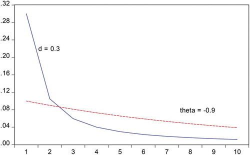
For particular values of $\theta$ and d, the patterns of the autoregressive parameters of the IMA(1,1) and the fractionally integrated process can look very similar. Consider for example Figure 1 which gives the first 10 autoregressive parameters, that is ${\alpha }_1$ to ${\alpha }_{10}$ for $\theta =-0.9$ and $d=0.3$.

Figure 1. The first 10 autoregressive parameters in an approximate autoregressive model, that is ${\alpha }_1$ to ${\alpha }_{10}$ for $\theta =-0.9$ and $d=0.3$.

IV. Conclusion

In this note, I proposed to replace the random walk benchmark model in forecast evaluations by another model, which has more face value for many economic variables. This new benchmark model is the Integrated Moving Average model of order (1,1). I have put forward six arguments why this IMA(1,1) model is a suitable benchmark model in practice.

Disclosure statement

No potential conflict of interest was reported by the author.

References

- Assimakopoulos, V., and K. Nikolopoulos. 2000. “The Theta Model: A Decomposition Approach to Forecasting.” International Journal of Forecasting 16: 521–530. doi:10.1016/S0169-2070(00)00066-2.
- Chatfield, C. 1993. “Calculating Interval Forecasts (With discussion).” Journal of Business and Economic Statistics 11: 121–144.
- Chatfield, C., A. B. Koehler, J. K. Ord, and R. D. Snyder. 2001. “A New Look at Models for Exponential Smoothing.” The Statistician 50: 146–159.
- Franses, P. H., D. van Dijk, and A. Opschoor. 2014. Time Series Models for Business and Economic Forecasting. Cambridge UK: Cambridge University Press.
- Granger, C. W. J. 1980. “Long Memory Relationships and the Aggregation of Dynamic Models.” Journal of Econometrics 14: 227–238. doi:10.1016/0304-4076(80)90092-5.
- Granger, C. W. J., and N. Hyung. 2004. “Occasional Structural Breaks and Long Memory with an Application to the S&P 500 Absolute Stock Returns.” Journal of Empirical Finance 11: 399–421. doi:10.1016/j.jempfin.2003.03.001.
- Granger, C. W. J., and R. Joyeux. 1980. “An Introduction to Long-memory Time Series Models and Fractional Differencing.” Journal of Time Series Analysis 1: 15–39. doi:10.1111/j.1467-9892.1980.tb00297.x.
- Harvey, A. C. 1989. Forecasting, Structural Time Series Models and the Kalman Filter. Cambridge UK: Cambridge University Press.
- Harvey, A. C., and S. J. Koopman. 2000. “Signal Extraction and the Formulation of Unobserved Components Models.” Econometrics Journal 3: 84–107. doi:10.1111/1368-423X.00040.
- Hyndman, R. J., and B. Billah. 2003. “Unmasking the Theta Method.” International Journal of Forecasting 19: 187–290. doi:10.1016/S0169-2070(01)00143-1.
- Kim, H. H., and N. R. Swanson. 2018. “Mining Big Data Using Parsimonious Factor, Machine Learning, Variable Selection and Shrinkage Methods.” International Journal of Forecasting 34: 339–354. doi:10.1016/j.ijforecast.2016.02.012.
- Makridakis, S., and M. Hibon. 2000. “The M3-competitions: Results, Conclusions and Implications.” International Journal of Forecasting 16: 451–476. doi:10.1016/S0169-2070(00)00057-1.
- Makridakis, S., E. Spiliotis, and V. Assimakopoulos. 2019. “The M4 Competition: 100,000 Time Series and 61 Forecasting Methods.” International Journal of Forecasting. in print. doi:10.1016/j.ijforecast.2019.04.14.
- Nelson, C. R., and C. I. Plosser. 1982. “Trends and Random Walks in Macroeconomic Time Series: Some Evidence and Implications.” Journal of Monetary Economics 10: 139–162. doi:10.1016/0304-3932(82)90012-5.
- Rossana, R., and J. Seater. 1995. “Temporal Aggregation and Economic Time Series.” Journal of Business and Economic Statistics 13: 441–451.
- Working, H. 1960. “Note on the Correlation of First Differences of Averages in a Random Chain.” Econometrica 28: 916–918. doi:10.2307/1907574.