Testing the accruals anomaly based on the speed of price adjustment

Abstract

In this study, we investigate the nature of the accruals anomaly by analyzing the speed of price adjustment to accruals information. Consistent with the mispricing hypothesis, we find that a relatively larger proportion of accruals premium is distributed near the filing dates among low limits-to-arbitrage stocks and during periods of increased arbitrage activity. We also discuss our findings in the context of q-theory.

KEYWORDS:

• Accruals anomaly
• market efficiency
• limits to arbitrage
• mispricing
• Q-theory of investment

JEL Numbers:

• G02
• G10
• G12
• G14

1. Introduction

Previous research shows that profits to accruals-based trading strategies vary across firms or time periods (e.g. Mashruwala, Rajgopal, and Shevlin 2006; Richardson, Tuna, and Wysocki 2010; Green, Hand, and Soliman 2011). However, it is unclear how the initial returns near the date when accruals information becomes publicly known compare to the later returns. Knowing the time distribution of accruals premium starting from the information release date is important because it will shed light on the nature of the accruals anomaly. In this study, we investigate the nature of the accruals anomaly by analyzing the speed of price adjustment to accruals information (i.e. the time distribution of accruals premium).

The accruals anomaly refers to the negative relation between accruals and subsequent stock returns. The literature has traditionally interpreted the accruals anomaly as being driven by mispricing (e.g. Sloan 1996; Hirshleifer, Teoh, and Yu 2011). These studies generally imply that investors do not respond properly to the mispricing signal in accruals at the time of release, thus inducing a negative relation between accruals and subsequent stock return. More recently, Wu, Zhang, and Zhang (2010) offer an alternative explanation based on the q-theory of investment.¹ They argue that firms optimally adjust their accruals (i.e. working capital investments) in response to discount rate changes and that the predictable subsequent returns associated with accruals reflect rationally expected discount rates. Empirically, they show that the q-theory approach can accommodate most of the existing evidence for the mispricing hypothesis without assuming investor irrationality. Evaluated in light of their findings, the existing evidence is at best inconclusive on the mechanism of the accruals anomaly. This necessitates new research on the nature of the anomaly.

The speed of price adjustment (i.e. the time distribution of the ‘accruals premium’ starting from the release of accruals information) provides important information for evaluating the mispricing hypothesis.² Several studies attempt to support the mispricing hypothesis by showing that anomalous returns to accruals-based trading strategies are smaller among low limits-to-arbitrage stocks or after sophisticated investors learn about the strategy (e.g. Mashruwala, Rajgopal, and Shevlin 2006; Richardson, Tuna, and Wysocki 2010; Green, Hand, and Soliman 2011). These authors interpret their findings as evidence that more arbitrage causes the mispricing signals to be incorporated into stock prices faster, thus resulting in a smaller anomalous return after the portfolio formation date. This argument implies that the decrease in anomalous return after the portfolio formation date should be accompanied by an increase in anomalous return before the portfolio formation date, especially during the period surrounding the release of accruals information. Yet, based on the existing literature, it is unclear whether a corresponding increase in accruals premium exists near the accruals information release date. As we discuss later, without examining the stock return around the release of accruals information, the evidence in these studies could also be explained by different versions of the q-theory of investment. In other words, prior research provides incomplete evidence to support the mispricing hypothesis.

Measuring the accruals premium starting from the information release date also provides useful information for evaluating the q-theory based explanation. While the return realized between the information release date and the portfolio formation date is also part of the accruals premium, the existing literature does not relate it to later returns. For example, Wu, Zhang, and Zhang (2010) measure the accruals premium from the portfolio formation date and attribute the decay of the accruals anomaly in recent years to time varying discount rate. However, the anomalous return after the portfolio formation date may decrease because increased arbitrage causes the accruals-related stock return effects to be realized before the portfolio formation date. It is not clear, therefore, whether the accruals premium has indeed decreased, as Wu, Zhang, and Zhang (2010) suggest, if the accruals premium earned before the portfolio formation date is taken into consideration.

Specifically, we examine how the speed of price adjustment to accruals information varies with the cross-sectional and time series variations in arbitrage activities. We base our inferences about the speed of price adjustment on the results of the following three tests. In the first test, we examine the stock market reactions surrounding 10 K/Q filing dates, when most firms release the information necessary for calculating quarterly accruals.³ A significantly negative relation between accruals and filing return will be evidence of immediate stock market response to accruals information. In the second test, we examine the relation between next-quarter stock return and current- and last-quarter accruals. If investors respond more promptly to accruals information, the accruals premium will be realized sooner after the 10 K/Q filing dates. This means that accruals will have more predictive power for stock return in the near future relative to their predictive power for stock return in the more distant future. Therefore, with faster price adjustment, the correlation of next-quarter stock return with current-quarter accruals should be stronger relative to its correlation with last-quarter accruals. In the third test, we examine the trading behavior of a group of sophisticated market participants – short sellers. If short sellers respond promptly to accruals information, we should observe a significant increase in short interest for high accruals stocks around the 10 K/Q filing month.

We use these three tests to investigate how the variation in arbitrage activity affects the speed of price adjustment to accruals information. In the first part of the paper, we exploit the cross-sectional variation in limits to arbitrage. According to the mispricing hypothesis, limits to arbitrage discourage investors from engaging in arbitrage activities aimed at exploiting the mispricing signals in accruals. Therefore, the mispricing hypothesis predicts faster price adjustment to accruals information for easy-to-arbitrage stocks.

Consistent with this view, we find that the relation between accruals and filing return is significantly more negative for the tercile of firms with low limits to arbitrage than for the tercile with high limits to arbitrage. Moreover, we find that current-quarter accruals and last-quarter accruals have statistically indistinguishable predictive power for next-quarter stock return in the high limits-to-arbitrage group. By contrast, in the low limits-to-arbitrage group, last quarter accruals have significantly lower predictive power for next quarter stock return than current quarter accruals do. In addition, our short interest test results indicate that short sellers adjust their short positions immediately after observing easy-to-arbitrage stocks moving into the top accruals decile. By contrast, we do not detect a statistically significant increase in short interest surrounding the month when difficult-to-arbitrage stocks move into the top accruals decile.

Because proxies for limits to arbitrage are highly correlated with proxies for investment frictions, a version of the q-theory that incorporates investment frictions may explain why the magnitude of the accruals anomaly is larger for stocks with high investment frictions/limits to arbitrage (Lam and Wei 2011; Lam et al. 2020; Li and Zhang 2010). However, our findings are inconsistent with the q-theory with investment frictions. First, from the q-theory perspective, the relation between accruals and filing return should be non-negative for both low and high limits-to-arbitrage/investment friction stocks.⁴ Yet, we document a significantly negative relation between accruals and filing return for low limits-to-arbitrage/investment friction stocks. Second, according to the q-theory with investment frictions, high investment friction stocks should earn a larger accruals premium than low investment friction firms. However, we find that high limits-to-arbitrage/investment friction stocks earn a smaller accruals premium than low limits-to-arbitrage/investment friction stocks in the first quarter starting from filing. Over a two-quarter horizon, high limits-to-arbitrage/investment friction stocks also do not earn a larger accruals premium than low limits-to-arbitrage/investment friction stocks.⁵

In further analysis, we examine how the time variation in arbitrage activity relates to the speed of price adjustment to accruals information. Following previous research, we divide our sample period into three sub-periods, which we refer to as the pre-arbitrage period (1988–1994), the low-arbitrage period (1995–2002), and the high-arbitrage period (2003–2018).⁶ Previous research suggests that accruals-based arbitrage activity has increased in recent years due to increased liquidity (Chordia, Subrahmanyam, and Tong 2014) and adaptive learning by investors (Richardson, Tuna, and Wysocki 2010; Green, Hand, and Soliman 2011). If the accruals anomaly is attributable to mispricing, increased arbitrage activity should lead to faster price adjustment to accruals information in the more recent period.

Consistent with the mispricing hypothesis, we find a significantly negative relation between accruals and filing return during the high-arbitrage period, but not during the low-arbitrage period. Moreover, for the pre-arbitrage and low-arbitrage periods, current-quarter accruals and last-quarter accruals have statistically indistinguishable predictive power for next-quarter stock return. For the high-arbitrage period, we find that last-quarter accruals have less than 6% the predictive power of current-quarter accruals for next-quarter stock return. These results suggest that the accruals premium is realized sooner after the filing dates in the high-arbitrage period than in the two earlier periods.⁷ In addition, our short interest test results show that short sellers adjust their short positions immediately after observing firms moving into the top accruals decile in the high-arbitrage period, but not in the pre-arbitrage and the low-arbitrage periods.

From the q-theory perspective, Wu, Zhang, and Zhang (2010) argue that the decay of anomalous return can be interpreted as reflecting the time variation in discount rates. Our findings are inconsistent with the time varying discount rate argument. First, according to the q-theory, there should be either no relation or a positive relation between accruals and filing return in all three periods, depending on whether the discount rate information in accruals is anticipated or not. However, we find a significantly negative relation between accruals and filing return in the high-arbitrage period. Second, if the decay of the accruals-related anomalous return reflects the time variation in discount rates, the accruals premium should be smaller in the high-arbitrage period than in the pre-arbitrage and the low-arbitrage periods. However, when we measure accruals premium from the filing date, we find that the accruals premium in the first quarter following filing is larger, rather than smaller, in the high-arbitrage period than in the previous two periods. Additionally, over a two-quarter horizon, the accruals premium is statistically indistinguishable across the pre-arbitrage, low-arbitrage and high-arbitrage periods.

We emphasize that the focus of our tests is on the speed of price adjustment (i.e. the time distribution of accruals premium) rather than on the return magnitude. Although the existing literature suggests that anomaly returns tend to be smaller when there are more arbitrage activities, we find that the accruals premium in the filing period and in the first quarter after filing is larger among low limits-to-arbitrage stocks and in the high-arbitrage period. However, these results should neither be interpreted as being inconsistent with previous research nor as evidence against the mispricing hypothesis. In order to track investors’ reaction to accruals information, we measure the accruals premium starting from the quarterly filing date rather than from a subsequent portfolio formation date. According to the mispricing hypothesis, arbitrage reduces the accruals anomaly (i.e. the anomalous return earned after the portfolio formation date) because it causes a larger proportion of accruals-related return effects to be realized before the portfolio formation date. In other words, arbitrage activities cause the accruals premium to be distributed closer to the filing date. Thus, if the mispricing hypothesis holds, it is natural for the accruals premium in the period immediately after filing to be larger among low limits-to-arbitrage stocks and in the high-arbitrage period. In terms of return magnitude, the mispricing hypothesis only predicts that arbitrage reduces the anomalous return after the portfolio formation date, but does not predict that arbitrage reduces the accruals premium starting from the release date of the accruals information.

Overall, the evidence documented in this study suggests that arbitrage activities affect the time distribution of the accruals premium rather than the size of the accruals premium. Although many researchers interpret the accruals anomaly as being driven by mispricing, the q-theory approach can accommodate most of the previous evidence that has been used to support this interpretation. For example, although previous research has examined how limits to arbitrage affect the accruals anomaly (e.g. Li and Sullivan 2011; Mashruwala, Rajgopal, and Shevlin 2006), the evidence in these studies cannot differentiate between the mispricing hypothesis with limits to arbitrage and q-theory with investment frictions. Based on the speed of price adjustment, we provide evidence that is more consistent with the mispricing hypothesis than with the existing versions of the q-theory. We caution readers that, while our findings seem most consistent with mispricing, like all similar studies, new extensions of q-theory may emerge to account for these patterns as our understanding of the returns to risk evolves.

Our empirical strategy of comparing initial and later returns is intuitively appealing. Whereas the q-theory concerns the magnitude of discount rates, the mispricing hypothesis is more precisely a hypothesis about price adjustment speed in initial and later periods. If accruals are observable mispricing signals, the accruals anomaly will occur only if investors fail to react properly to the mispricing signals at the time of their release. Thus, the time distribution of accruals premium after the filing date contains important information about the nature of the accruals anomaly. In the accruals anomaly literature, Battalio et al. (2012) study initial returns around filing dates and Sloan (1996) studies the concentration of anomalous returns around future earnings announcements. In a contemporaneous study, Bowles et al. (2020) examine the speed of price adjustment of a broad cross-section of anomalies and test whether anomalies are spurious. Although strategies similar to ours have been used to study the post-earnings announcement drift (Bernard and Thomas 1989; Zhang 2008), the strategy of comparing initial and later returns remain largely under-exploited in the existing accruals anomaly literature. Our study shows that additional insights into the nature of stock market anomalies can be gained by analyzing the speed of price adjustment.

2. Related research

Sloan (1996) finds that firms with high accruals earn lower abnormal future stock returns than firms with low accruals. From the mispricing perspective, a large number of studies argue that the accruals anomaly occurs because investors overestimate the persistence of accruals (e.g. Sloan 1996) or because they misunderstand the relation between future profitability and growth, which is closely correlated with accruals (e.g. Fairfield, Whisenant, and Yohn 2003; Cooper, Gulen, and Schill 2008). Other studies offer rationality-based explanations for the accruals anomaly. For example, Khan (2008) argues that a considerable portion of the cross-sectional variation in average returns to high and low accruals firms is explained by risk. More recently, Wu, Zhang, and Zhang (2010) offer an explanation based on the q-theory of investment. They argue that accruals predict subsequent stock returns because firms optimally adjust their accruals in response to discount rate changes.

The q-theory approach offers several advantages over consumption-based asset pricing models in explaining the accruals anomaly. Theoretically, it models the interaction between discount rate and accruals, whereas the consumption-based models are silent on why high accruals firms are characterized with lower risk. Empirically, the q-theory approach can accommodate most of the previous evidence on the accruals anomaly. For example, previous research shows that the magnitude of the accruals anomaly is larger among high limits-to-arbitrage stocks (Li and Sullivan 2011; Mashruwala, Rajgopal, and Shevlin 2006). Though often viewed as supporting the mispricing hypothesis, the evidence is also consistent with the q-theory with investment frictions. According to the q-theory, firms make more investments, including working capital investments, when discount rates are lower. In the presence of investment frictions, making new investment incurs deadweight loss. Because deadweight loss partially offsets the net present value generated from investment activities, firms with high investment frictions are reluctant to invest even when the discount rate is lower. Thus, the investment friction hypothesis predicts that the accruals anomaly is stronger for firms with high investment frictions than for firms with low investment frictions. However, the proxies for limits to arbitrage are highly correlated with the proxies for investment frictions (Lam and Wei 2011; Lam et al. 2020). Many limits-to-arbitrage measures, such as illiquidity and market value of equity, could also be interpreted as capturing the cross-sectional variation in financing and investment frictions. As a result, if the accruals anomaly is found to be stronger among firms with high values of these measures, the evidence could be explained by either the mispricing hypothesis with limits to arbitrage or the q-theory with investment frictions.

As another example, Richardson, Tuna, and Wysocki (2010) and Green, Hand, and Soliman (2011) find that the returns to accruals-based hedge portfolios have attenuated in recent years. They interpret their findings as evidence that capital market participants have learned about mispricing signals in accruals and arbitraged away the anomaly. However, from the q-theory perspective, the decay in the accruals anomaly in recent years can be explained by the time-varying discount rate explanation, in which the expected returns associated with accruals portfolios can also vary.

The q-theory approach can accommodate evidence that cannot be easily explained by the traditional consumption-based models. For example, it can explain why accruals-related stock return effects are concentrated around subsequent earnings announcements (Sloan 1996). While this evidence is often viewed as a hurdle for risk-based explanations, it can be explained from the q-theory perspective because investment-based asset pricing predicts the concentration of ex post realizations of returns around subsequent earnings announcements (Wu, Zhang, and Zhang 2010).

More broadly, the q-theory approach has been used to explain the predictable return associated with equity issuance, book-to-market ratio, capital investment, and many other firm characteristics (e.g. Lyandres, Sun, and Zhang 2008; Liu, Whited, and Zhang 2009). Hou, Xue, and Zhang (2015) propose a four-factor model based on the q-theory of investment. They show that their model’s performance is at least comparable to, and in many cases better than, that of the Fama-French (1993) 3-factor model and the Carhart (1997) 4-factor model in capturing the remaining significant anomalies.

3. Empirical strategy

To explore the nature of the accruals anomaly, we examine how the speed of price adjustment to accruals information varies with the cross-sectional and time series variations in arbitrage activities. Using Figures 1 and 2, we illustrate the advantages of focusing on the speed of price adjustment to accruals information. Panels A and B of Figure 1 depict the cumulative returns of two low accruals stocks, starting from the 10 K/Q filing dates, as suggested by the mispricing hypothesis. With a more concave return trajectory, the stock in Panel A exhibits faster price adjustment than the stock in Panel B. That is, the stock in Panel A has a larger proportion of the accruals-related return effect realized near the filing date.

Figure 1. High vs. low speed of price adjustment. The figures depict the stock return trajectories for low accruals firms with different price adjustment speeds. Panel A depicts the return trajectory for a low accruals stock starting from the filing date, with fast speed of price adjustment. Panel B depicts that for an otherwise similar stock with slow speed of price adjustment. Panel C depicts the anomalous returns of the two stocks starting from the portfolio formation date. Panel A. Stock return starting from the filing date, high speed of price adjustment. Panel B. Stock return starting from the filing date, low speed of price adjustment. Panel C. Anomalous returns from the portfolio formation date.

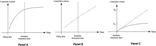
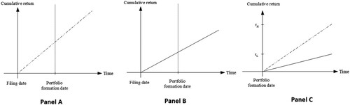
Figure 2. High vs. low investment frictions. The figures depict the stock return trajectories for low accruals firms with different investment frictions. Panel A depicts the return trajectory for a low accruals stock starting from the filing date, with high investment frictions. Panel B depicts that for an otherwise similar stock with low investment frictions. Panel C depicts the anomalous returns of the two stocks starting from the portfolio formation date. Panel A. Stock return starting from the filing date, high investment frictions. Panel B. Stock return starting from the filing date, low investment frictions. Panel C. Anomalous returns from the portfolio formation date.

According to the mispricing hypothesis, higher limits to arbitrage discourage market participants from trading on knowledge about mispricing signals at release time, which leads to slower price adjustment. Thus, we can think of the solid line in Panel A as representing a low accruals stock with low limits to arbitrage and the dashed line in Panel B as representing an otherwise similar stock with high limits to arbitrage. In Panel C, we re-draw the return trajectories of these two low accruals stocks, starting from a subsequent portfolio formation date (i.e. setting the portfolio formation date as the origin of the coordinate system). For the easy-to-arbitrage stock, a larger proportion of the accruals-related stock return effect is realized before the portfolio formation date. Hence, it tends to earn lower anomalous return after the portfolio formation date (i.e. R_H > R_L).

The q-theory of investment links accruals to the magnitude of discount rates. It predicts that firms invest more in working capital when discount rates are lower. Figure 2 presents the cumulative returns of two low accruals stocks, as suggested by the q-theory of investment. The magnitude of stock return (i.e. realized discount rate) is larger in Panel A than in Panel B. In the presence of high investment frictions, making new investment incurs deadweight loss, which partially offsets the net present value generated from investment activities. Therefore, firms with high investment frictions will require a higher discount rate to make the same level of working capital investment. We can think of Panel A as representing the realized discount rate of a high investment friction firm with low accruals and Panel B as representing the realized discount rate of a low investment friction firm with similar accruals. In Panel C, we re-draw the return trajectories of the two stocks, starting from the portfolio formation date. The high investment friction stock earns higher anomalous return, as conventionally measured, than the low investment friction stock with similar accruals (i.e. r_H > r_L).

The magnitude of anomalous return tends to be larger both for the stock with high limits to arbitrage (Figure 1 Panel C) and the stock with high investment frictions (Figure 2 Panel C). To the extent that limits-to-arbitrage proxies capture the cross-sectional variations in investment frictions, mispricing with limits to arbitrage and q-theory with investment frictions generate indistinguishable predictions about the magnitude of anomalous return. That is, if we find that a high limits-to-arbitrage/investment friction stock earns higher anomalous return than a low limits-to-arbitrage/investment friction stock, we are unable to differentiate between the mispricing hypothesis and the q-theory.

However, if we focus on the speed of price adjustment, the two hypotheses are clearly distinguishable. The low limits-to-arbitrage stock in Figure 1 Panel A exhibits faster price adjustment than the high limits-to-arbitrage stock in Figure 1 Panel B. The low limits-to-arbitrage stock has a larger proportion of accruals-related stock return effects distributed near the filing date. Thus, under the mispricing hypothesis with limits-to-arbitrage, it is possible for low limits-to-arbitrage/investment friction stocks to earn a larger accruals premium than high limits-to-arbitrage/investment friction stocks near the filing date.

In Figure 2 Panel A and Figure 2 Panel B, the high and low investment friction stocks differ not in price adjustment speed, but in the magnitudes of accruals premiums, which reflect the respective discount rates of the two stocks. The q-theory with investment frictions does not explain why low investment friction may cause the accruals premium to be distributed closer to the filing date. The stock return earned before the portfolio formation date is also part of the accruals premium. A low limits-to-arbitrage/investment friction stock should have a smaller accruals premium than a high limits-to-arbitrage/investment friction stock near the filing date or over the whole post-filing period (i.e. before and after the portfolio formation date).

Figures 1 and 2 can also be used to illustrate the advantages of studying how the speed of price adjustment to accruals information changes across time periods. The mispricing hypothesis predicts that increased arbitrage from increased liquidity (Chordia, Subrahmanyam, and Tong 2014) and adaptive learning by investors (Green, Hand, and Soliman 2011) will lead to faster price adjustment in the more recent period. In this context, we can think of Figure 1 Panel B as depicting the price adjustment process for a low accruals stock in the earlier years and Figure 1 Panel A as depicting the process in the more recent years. Wu, Zhang, and Zhang (2010) attribute the decay of the accruals anomaly to the time variation in discount rate. To be consistent with their view, we can think of Figure 2 Panel A as representing the realized discount rate of a low accruals stock in the earlier years, and Figure 2 Panel B as representing the realized discount rate of a similar stock in the more recent years. In Figure 1 Panel C and Figure 2 Panel C, we present the return trajectories of the stocks, starting from the portfolio formation date. A comparison of Figure 1 Panel C with Figure 2 Panel C shows that the mispricing hypothesis and the q-theory of investment generate indistinguishable predictions about the magnitude of anomalous return (i.e. R_H > R_L and r_H > r_L). However, if we focus on the speed of price adjustment, the two hypotheses are distinguishable, as indicated by the difference between Figures 1 and 2.

We draw on the conceptual framework in Figures 1 and 2 to develop our empirical strategy for testing the mispricing hypothesis against the q-theory of investment. In our first set of tests, we examine how the cross-sectional variation in arbitrage activity caused by the differences in limits to arbitrage affects the speed of price adjustment to accruals information. Specifically, we divide sample firms into terciles based on limits to arbitrage and test whether firms in the bottom limits-to-arbitrage tercile exhibit faster price adjustment than firms in the top tercile. In the second set of tests, we examine how the speed of price adjustment to accruals information changes across time periods. Specifically, we divide the sample period into three sub-periods: pre-arbitrage period (1988–1994), low-arbitrage period (1995–2002) and high-arbitrage period (2003–2018), and test whether investors respond more promptly to accruals information in the high-arbitrage period than in the two earlier periods.

The cutoff points between the sub-periods roughly correspond to those used in previous research. Before Sloan’s publication in 1996 (i.e. in the pre-arbitrage period), the accruals anomaly was little known among practitioners. Following Green, Hand, and Soliman (2011), we divide the post-1995 period into two sub-periods, which we refer to as the low-arbitrage period (1995–2002) and the high-arbitrage period (2003–2018). The high-arbitrage period (2003–2018) is likely to be characterized by more intense arbitrage activity than the low-arbitrage period (1995–2002) for the following two reasons. First, adaptive learning involves more than just being aware of the accruals anomaly. As argued by Bebchuk, Cohen, and Wang (2013), investor learning is a gradual process. It may take time for investors to digest information about the accruals anomaly, refine their accruals-based trading strategies, and raise the capital necessary to arbitrage on the anomaly. The effect of investor learning on the speed of price adjustment will manifest only when a sufficient number of market participants take actions to arbitrage. Given the gradual nature of the process, the effect of adaptive learning should be stronger in the more recent high-arbitrage period (2003–2018) than in the older low-arbitrage period (1995–2002).⁸ Second, increased liquidity in more recent years will stimulate more arbitrage activity (Chordia, Subrahmanyam, and Tong 2014).

We examine the speed of price adjustment to quarterly accruals information using the following three tests.⁹ The first test focuses on the short-term stock returns surrounding 10 K/Q filing dates, when most firms release the information necessary to calculate accruals. To assess investors’ immediate reactions to accruals information, we estimate the following regression model:¹⁰ (1) $CA{R}_{i,t}=\beta TAC{C}_{i,t}^{dec}+Controls+{\epsilon }_{i,t}$(1)

In Equation (1)(1) $CA{R}_{i,t}=\beta TAC{C}_{i,t}^{dec}+Controls+{\epsilon }_{i,t}$(1) , $TAC{C}_{i,t}^{dec}$ is the transformed accruals ranking for firm i in quarter t,¹¹ and $CA{R}_{i,t}$ is the market-adjusted buy-and-hold abnormal return (using the value-weighted CRSP index return as the benchmark market return) surrounding the date on which firm i files its 10 K/Q for quarter t. When $TAC{C}_{i,t}^{dec}$ is so defined, its coefficient can be interpreted as the return to a hedge portfolio that is long in stocks in the highest accruals decile and short in stocks in the lowest accruals decile. We control for size, book-to-market ratio, and standardized unexpected earnings (SUE) in our analysis.

More pronounced stock return reactions around the filing dates are evidence of faster price adjustment. To be consistent with the mispricing hypothesis, $\beta$ should be more negative in the low limits-to-arbitrage tercile than in the high limits-to-arbitrage tercile. It should also be more negative in the high-arbitrage period than in the two earlier periods. Finding a negative relation between accruals and filing return is not consistent with the q-theory of investment, which predicts that low accruals firms have higher discount rates. If accruals only contain information about rationally expected discount rates, the stock market will not respond. If low accruals provide market participants with information about unexpected increases in discount rates, investors will respond by revising the stock price downward. This implies a positive relation between accruals and filing return.

In our second test, we compare the predictive power of current and lagged accruals for next-quarter stock return. Specifically, we estimate the following model: (2) $BHA{R}_{i,t+1}=\beta TAC{C}_{i,t}^{dec}+\gamma TAC{C}_{i,t-1}^{dec}+Controls+{\epsilon }_{i,t}$(2) In Equation (2)(2) $BHA{R}_{i,t+1}=\beta TAC{C}_{i,t}^{dec}+\gamma TAC{C}_{i,t-1}^{dec}+Controls+{\epsilon }_{i,t}$(2) , $BHA{R}_{i,t+1}$ is the quarter-ahead return, defined as the market-adjusted buy-and-hold return measured from one day before the 10 K/Q filing date for quarter t to two days before the filing date for the subsequent quarter (i.e. t + 1). $TAC{C}_{i,t}^{dec}$ and $TAC{C}_{i,t-1}^{dec}$ are the transformed accruals decile rankings for firm i at the end of quarter t and quarter t − 1, respectively. We control for size, book-to-market ratio, and current and lagged standardized unexpected earnings. If investors react more promptly to accruals information, a larger proportion of the accruals premium should be realized soon after the filing date. Thus, faster adjustment speed implies that the correlation between accruals and stock returns near the filing date is stronger relative to the correlation between accruals and stock returns in the subsequent period. If the mispricing hypothesis holds, $\beta$ should be more negative relative to $\gamma$ in the easy-to-arbitrage group than in the difficult-to-arbitrage group. It should also be more negative relative to $\gamma$ in the high-arbitrage period than in the earlier periods. Moreover, under the mispricing hypothesis, it is possible for the high limits-to-arbitrage group to have a less negative $\beta$ than the low limits-to-arbitrage group because high limits-to-arbitrage stocks tend to have delayed responses to accruals information. In contrast, the q-theory of investment concerns the relation between accruals and return magnitude, rather than the relation between accruals and the speed of price adjustment. It does not predict that discount rates are realized faster for low investment friction firms or in the high-arbitrage period (2003–2018). $\beta$ and $\gamma$ can be interpreted as the accruals premium earned in the first and second quarters, respectively, after filing. To be consistent with the q-theory of investment, both $\beta$ and $\beta$+$\gamma$ should be more negative for high investment friction firms than for low investment friction firms. They should also be more negative in periods with high discount rates than in periods with low discount rates.

Lastly, we supplement our stock return tests with tests based on short sellers’ behavior. Using the following model, we estimate short sellers’ reactions to accruals information. (3) $\mathrm{\Delta }S{I}_{i,m}=\beta To{p}_{i,m}+Controls+{\epsilon }_{i,m}$(3)

In Equation (3)(3) $\mathrm{\Delta }S{I}_{i,m}=\beta To{p}_{i,m}+Controls+{\epsilon }_{i,m}$(3) , $\mathrm{\Delta }S{I}_{i,m}$ is the change in short interest for stock i surrounding filing month m. $To{p}_{i,m}$ is an indicator variable that equals one for stocks that move into the highest quarterly accruals decile in month m, and zero otherwise. We focus on the top accruals decile because the existing evidence of short arbitrage activity is confined mainly to the top accruals decile (Hirshleifer, Teoh, and Yu 2011). Following Hirshleifer, Teoh, and Yu (2011), we estimate the model using stocks that shift toward higher accruals deciles in month m.¹² If short sellers initiate or increase their short positions after observing firms shifting into the top accruals decile, $\mathrm{\Delta }S{I}_{i,m}$ should be positively related to $To{p}_{i,m}$. The changes in short interest should be more pronounced when more investors engage in arbitrage activities. Thus, the mispricing hypothesis predicts a more positive estimate of $\beta$ among low limits-to-arbitrage firms than among high limits-to-arbitrage firms. To be consistent with the mispricing hypothesis, $\beta$ should also be more positive in the high-arbitrage period than in the two earlier periods.

4. Data

We begin with all firm-quarter observations in the Compustat Fundamental Quarterly Database from Q1/1988 to Q4/2018.¹³ Previous research shows that quarterly accruals trading strategies that do not control for unexpected earnings will likely be understated (Collins and Hribar 2000). We therefore require that sample observations have sufficient data to compute both total accruals and standardized unexpected earnings. Following Hribar and Collins (2002), we compute total accruals using the Statement of Cash Flow approach: $Accrual{s}_t=(Earning{s}_t-CF{O}_t)/Averagetotalassets$where $Earning{s}_t$ is earnings from continuing operations (Compustat item: IBQ), and $CF{O}_t$ is cash flow from continuing operations, which is computed from Compustat item OANCFY. Following Richardson, Tuna, and Wysocki (2010), we compute standardized unexpected earnings as the seasonally differenced return on average assets divided by the rolling 12-quarter standard deviation of this seasonal difference. We require that the sample observations have fiscal quarters ending in March, June, September, and December.¹⁴

We then match the accounting data with stock return data from CRSP. We require that sample firms have CRSP share codes of 10 or 11, be listed on the NYSE, NASDAQ or AMEX, and have stock prices above $1 at the fiscal quarter end. Our short interest data are from Compustat and Factset.¹⁵ We calculate CAR, BHAR, and the short interest variables as described in Section 2.¹⁶ When we calculate BHAR for delisted firms, we include the delisting returns from CRSP and invest the proceeds in a size-matched portfolio.

Because our goal is to assess the speed of price adjustment, we measure stock return starting from one day before the 10 K/Q filing date. We obtain the 10 K/Q filing dates for observations between Q1/1995 and Q2/2009 from Amir Sufi’s website,¹⁷ and identify the filing dates for observations between Q3/2009 and Q4/2018 from the SEC website. We exclude late filings by applying several filters. Specifically, we exclude firm-quarter observations when (1) there is a late filing report (Form NT 10-Q or Form NTN 10-Q) between the filing date and the fiscal quarter end; (2) the filing date is later than the Compustat reported earnings announcement date (RDQ) for the following quarter; or (3) the filing date is 90 days after the earnings announcement date for the fiscal quarter.

When we compare the speed of price adjustment between low and high limits-to-arbitrage stocks, our sample consists of firm-quarter observations from Q2/1995 to Q4/2018, for which actual filing dates are known.¹⁸ When we compare the speed of price adjustment across sample periods, our quarter-ahead return test and short interest test include firm-quarter observations from Q1/1988 to Q4/2018. Since actual filing dates are not available before 1995, we calculate quarter-ahead stock returns and short interest changes for the pre-arbitrage period based on estimated filing dates. Following Collins and Hribar (2000), we estimate filing dates in the pre-learning period to be 15 days after the earnings announcement dates.¹⁹

Table 1 presents descriptive statistics for the sample. The mean (median) total accruals is −0.0133 (−0.0094) and the mean (median) standardized unexpected earnings is −0.1997 (−0.0019). The mean (median) market value of equity is $4,109.92 (327.63) million and the mean (median) book-to-market ratio is 0.6789 (0.5328). Because precise information about filing dates is not available until 1995, we are able to calculate filing period returns for only 229,854 observations. Average cumulative abnormal returns over the (−1, 2), (−1, 5) and (−1, 10) windows around the 10 K/Q filing date are −0.0018, −0.0017 and −0.0008, respectively. We calculate changes in short interest ($\mathrm{\Delta }S{I}_1$) and quarter-ahead stock returns $(BHAR)$ based on both actual and estimated filing dates. Based on actual filing dates, the mean (median) $BHAR$ is 0.0020 (−0.0099) and $\mathrm{\Delta }S{I}_1$ is 0.0062 (0.0000). The mean and median statistics for $BHAR$ and $\mathrm{\Delta }S{I}_1$ calculated based on estimated filing dates are quite similar to the values obtained when actual filing dates are used, which indicates that there are unlikely to be systematic biases in the Collins and Hribar (2000) method we use for estimating filing dates.

Table 1. Descriptive statistics.

	N	Mean	Median	STD
TACC	275,559	−0.0133	−0.0094	0.1430
BM	275,559	0.6789	0.5328	0.6584
MV	275,559	4109.92	327.63	21395.35
SUE	275,559	−0.1997	−0.0019	13.1146
$\mathrm{\Delta }\text{S}{\text{I}}_1$	228,737	0.0062	0.0000	0.9647
$\mathrm{\Delta }{\text{SI}}_1^{est}$	264,862	0.0076	0.0000	0.8870
CAR(−1, 2)	229,854	−0.0018	−0.0026	0.0674
CAR(−1, 5)	229,854	−0.0017	−0.0032	0.0820
CAR(−1, 10)	229,854	−0.0008	−0.0036	0.1005
BHAR	229,837	0.0020	−0.0099	0.2209
$\text{BHA}{\text{R}}^{est}$	275,558	0.0018	−0.0103	0.2163
TURNOVER	274,650	1.6494	1.0472	2.2901
AMIHUD (*10^−6)	274,650	3.6282	0.0250	36.7567
HELD	275,558	0.4952	0.5035	0.3088

This table provides descriptive statistics for the sample employed in our analysis. The full sample consists of 275,559 firm-quarter observations from 1988 to 2018. Firms with stock prices below $1 and firms that are not listed on the NYSE, NASDAQ or AMEX are excluded. $TACC$ is quarterly accruals. $SUE$ is standardized earnings surprise. $MV$ is the market value of equity in millions of USD. $BM$ is the book-to-market ratio. $\mathrm{\Delta }S{I}_1$ is the change in short interest using monthly data around 10 K/Q filing dates. $\mathrm{\Delta }S{I}_1^{est}$ is the change in short interest around estimated filing dates. CAR(−1, 2), CAR(−1, 5) and CAR(−1, 10) are cumulative market-adjusted returns over the (−1, 2), (−1, 5) and (−1, 10) windows surrounding 10 K/Q filing dates, respectively. BHAR is quarter-ahead market-adjusted abnormal returns calculated based on actual filing dates. $BHA{R}^{est}$ is quarter-ahead market-adjusted abnormal returns calculated based on estimated filing dates. TURNOVER is turnover ratio. AMIHUD is Amihud illiquidity measure. HELD is institutional ownership. Detailed definitions for all variables are provided in Appendix A.

5. Results

According to the mispricing hypothesis, arbitrage activity leads to faster price adjustment. With faster price adjustment, a larger proportion of the accruals premium will be realized nearer the filing date. To test this conjecture, we investigate how the cross-sectional and time series variation in arbitrage activity relates to the distribution of the accruals premium.

5.1. Tests based on the cross-sectional variation in limits to arbitrage

We divide the sample firms into terciles each quarter based on each of the following limits-to-arbitrage measures: turnover ratio (TURNOVER), Amihud illiquidity measure (AMIHUD), institutional ownership (HELD), and market value of equity (MV).²⁰ We then compare the speed of investors’ reactions between the low and the high limits-to-arbitrage groups based on the results of filing return tests, quarter-ahead return tests, and short interest tests. If the mispricing hypothesis holds, the low limits-to-arbitrage group should exhibit faster investor reaction to accruals information.

5.1.1. Results from filing return tests

For the filing return tests, we estimate the model in Equation (1)(1) $CA{R}_{i,t}=\beta TAC{C}_{i,t}^{dec}+Controls+{\epsilon }_{i,t}$(1) , which uses market-adjusted cumulative returns over the (−1, 2), (−1, 5) and (−1, 10) windows surrounding the filing date as the dependent variables and TACC^dec, Log(MV), Log(BM) and SUE^dec as explanatory variables. TACC^dec and SUE^dec are the transformed decile rankings of total accruals and standardized unexpected earnings, respectively. Unless otherwise stated, all regression models in this study are estimated using the Fama and MacBeth (1973) procedure and t-statistics are calculated based on Newey-West adjusted standard errors.²¹

Table 2 compares the filing return test results between the low and the high limits-to-arbitrage terciles. In Panels A to D, we measure limits to arbitrage by turnover ratio, Amihud measure, institutional ownership, and market value of equity, respectively. In all panels, we report the results for easy-to-arbitrage stocks (i.e. stocks with high turnover ratio, low Amihud illiquidity measure, high institutional ownership, or large market capitalization) on the left and the corresponding results for difficult-to-arbitrage stocks on the right. In all panels and for all event windows, the coefficients for TACC^dec are significantly negative in the low limits-to-arbitrage groups. For example, in Column (1), the coefficient for TACC^dec is −0.0085, which is 4.41 standard errors away from zero. This suggests that high turnover stocks in the lowest accruals decile earn 0.85% more than those in the highest accruals decile over the (−1, +2) event window.

Table 2. Filing return tests for limits-to-arbitrage terciles.

	(1)	(2)	(3)	(4)	(5)	(6)	(7)	(8)	(9)	(10)	(11)	(12)
Measures	Panel A: TURNVOER						Panel B: AMIHUD
Limits of arbitrage	Low group (high TURNOVER)			High group (low TURNOVER)			Low group (low AMIHUD)			High group (high AMIHUD)
Event windows:	(−1,2)	(−1,5)	(−1,10)	(−1,2)	(−1,5)	(−1,10)	(−1,2)	(−1,5)	(−1,10)	(−1,2)	(−1,5)	(−1,10)
Intercept	−0.0154	−0.0172	−0.0159	−0.0062	−0.0069	−0.0075	−0.0026	−0.0029	−0.0011	−0.0106	−0.0116	−0.0144
	(−5.88)	(−5.08)	(−3.24)	(−4.22)	(−3.14)	(−2.33)	(−0.90)	(−0.65)	(−0.17)	(−4.08)	(−3.38)	(−3.35)
TACC^dec ($\beta$)	−0.0085	−0.0109	−0.0132	0.0004	−0.0015	−0.0018	−0.0076	−0.0086	−0.0102	0.0020	0.0004	0.0005
	(−4.41)	(−4.83)	(−4.98)	(0.30)	(−1.00)	(−1.10)	(−4.44)	(−4.58)	(−4.58)	(1.69)	(0.28)	(0.27)
Log(BM)	0.0018	0.0022	0.0020	0.0020	0.0032	0.0026	0.0005	0.0009	0.0009	0.0033	0.0045	0.0042
	(3.15)	(2.86)	(1.92)	(3.98)	(4.82)	(2.99)	(1.06)	(1.50)	(1.08)	(6.30)	(5.90)	(4.42)
Log(MV)	0.0022	0.0024	0.0022	0.0011	0.0015	0.0018	0.0004	0.0005	0.0004	0.0018	0.0022	0.0030
	(6.12)	(5.57)	(3.83)	(3.68)	(3.35)	(2.94)	(1.30)	(1.13)	(0.54)	(3.12)	(2.81)	(3.20)
SUE^dec	0.0177	0.0187	0.0206	0.0239	0.0280	0.0363	0.0104	0.0112	0.0126	0.0304	0.0349	0.0443
	(8.57)	(7.87)	(7.60)	(15.91)	(14.38)	(15.41)	(6.71)	(5.67)	(5.21)	(19.71)	(18.02)	(17.82)
Avg Adj-R^2	0.0175	0.0191	0.0190	0.0217	0.0238	0.0269	0.0159	0.0207	0.0241	0.0220	0.0220	0.0239
T-test:
${\beta }_{Low}-{\beta }_{High}=0$	−5.01	−4.27	−4.59				−5.84	−4.63	−4.46
	(13)	(14)	(15)	(16)	(17)	(18)	(19)	(20)	(21)	(22)	(23)	(24)
Measures	Panel C: HELD						Panel D: MV
Limits to arbitrage	Low group (high HELD)			High group (low HELD)			Low group (high MV)			High group (low MV)
Event windows:	(−1,2)	(−1,5)	(−1,10)	(−1,2)	(−1,5)	(−1,10)	(−1,2)	(−1,5)	(−1,10)	(−1,2)	(−1,5)	(−1,10)
Intercept	−0.0009	0.0017	0.0047	−0.0098	−0.0110	−0.0138	−0.0011	−0.0017	0.0004	−0.0117	−0.0124	−0.0153
	(−0.40)	(0.50)	(0.98)	(−5.09)	(−4.25)	(−4.21)	(−0.37)	(−0.38)	(0.06)	(−4.66)	(−4.36)	(−4.21)
TACC^dec ($\beta$)	−0.0098	−0.0128	−0.0154	0.0025	0.0014	0.0013	−0.0069	−0.0079	−0.0092	0.0011	−0.0009	−0.0006
	(−5.72)	(−7.09)	(−7.93)	(2.02)	(1.01)	(0.82)	(−4.61)	(−4.88)	(−4.66)	(0.94)	(−0.61)	(−0.36)
Log(BM)	0.0009	0.0011	0.0004	0.0032	0.0043	0.0045	0.0004	0.0008	0.0006	0.0031	0.0041	0.0041
	(1.82)	(1.72)	(0.48)	(7.19)	(6.30)	(5.03)	(0.80)	(1.15)	(0.66)	(6.18)	(6.15)	(4.94)
Log(MV)	0.0003	0.0000	−0.0004	0.0015	0.0019	0.0028	0.0002	0.0004	0.0002	0.0021	0.0023	0.0032
	(1.08)	(0.03)	(−0.76)	(3.83)	(3.75)	(4.52)	(0.73)	(0.80)	(0.24)	(3.64)	(3.53)	(3.95)
SUE^dec	0.0136	0.0149	0.0165	0.0288	0.0326	0.0414	0.0096	0.0107	0.0118	0.0323	0.0375	0.0470
	(5.92)	(6.00)	(6.16)	(20.96)	(20.22)	(18.48)	(6.41)	(5.66)	(5.23)	(20.25)	(19.87)	(19.20)
Avg Adj-R^2	0.0150	0.0187	0.0225	0.0208	0.0205	0.0229	0.0140	0.0202	0.0229	0.0219	0.0206	0.0222
T-test:
${\beta }_{Low}-{\beta }_{High}=0$	−7.44	−7.30	−6.99				−4.94	−3.70	−3.66

This table reports coefficients from the Fama and MacBeth (1973) regressions of filing period cumulative abnormal returns (CAR) on the independent variables shown. Panels A, B, C and D present the estimation results for low and high limits-to-arbitrage stocks, as measure by TURNOVER, AMIHUD, HELD and MV, respectively. TACC^dec is the decile ranking of quarterly accruals, which is transformed to a value between −0.5 and 0.5. Log(MV) is the log of market value of equity. Log(BM) is the log of book-to-market ratio. SUE^dec is the transformed decile ranking of standardized earnings surprise. TURNVOER is turnover ratio. AMIHUD is Amihud illiquidity measure. HELD is institutional ownership. MV is market value of equity. Definitions for all variables are provided in Appendix A. The t-statistics in parentheses are calculated using Newey-West standard errors. We use Welch’s unequal variances t-test to test the equivalence of coefficients between the high and the low limits-to-arbitrage groups.

For the high limits-to-arbitrage groups, the coefficient estimates for TACC^dec are statistically insignificant except in Columns (10) and (16). In Columns (10) and (16), the coefficients of TACC^dec are positive and statistically significant at the 5% or 10% levels. At first sight, it can be argued that these results are consistent with the q-theory because the q-theory predicts that there should be either no relation or a positive relation between accruals and filing return, depending on whether the discount rate information in accruals is anticipated or not. However, if the q-theory based explanation holds, the relation between accruals and filing return should also be non-negative for low limits-to-arbitrage stocks. Yet, we document a significantly negative relation between accruals and filing return for low limits-to-arbitrage stocks.

The results regarding low and high limits-to-arbitrage stocks can be simultaneously explained based on the mispricing hypothesis. From the mispricing perspective, these results indicate that the prices of easy-to-arbitrage stocks respond in the right direction to the mispricing signals in accruals around the filing dates, but the prices of difficult-to-arbitrage stocks initially do not respond or respond in the wrong direction. Battalio et al. (2012) find that investors who initiate very large trades (at least 5,000 shares) act almost immediately to exploit the information in accrual levels, while those who initiate very small trades (fewer than 500 shares) seem to react in the wrong direction. Because institutional investors generally prefer larger and more liquid stocks, their findings are potentially consistent with the positive coefficients of TACC^dec we document in Column (10) for stocks with high Amihud ratios and in Column (16) for those with low institutional holdings.

We formally test the equivalence of $\beta$ between the high and low limits-to-arbitrage groups. We use the Fama and MacBeth (1973) procedure to obtain a time series of estimated $\beta$’s for each tercile and then use Welch's unequal variances t-test to test whether the means of the time series for the low limits-to-arbitrage group are equal to the corresponding values for the high limits-to-arbitrage group, assuming unequal variances across the groups. The t-statistics reported at the bottom of the panels range from −3.66 to −7.44, indicating that the estimated values of $\beta$ are significantly more negative in the low limits-to-arbitrage groups than in the high limits-to-arbitrage groups. Consistent with the mispricing hypothesis, the Welch’s t-test results confirm that low limits-to-arbitrage stocks respond more promptly to accruals information.

5.1.2. Results from quarter-ahead return tests

In this section, we analyze how limits to arbitrage affect the relation between current-quarter accruals, lagged-quarter accruals, and next-quarter stock return. Our goal is to investigate whether the prices of easy-to-arbitrage stocks adjust more promptly to accruals information by estimating the model in Equation (2)(2) $BHA{R}_{i,t+1}=\beta TAC{C}_{i,t}^{dec}+\gamma TAC{C}_{i,t-1}^{dec}+Controls+{\epsilon }_{i,t}$(2) . The mispricing hypothesis with limits to arbitrage predicts that $\beta$ will be more negative relative to $\gamma$ among low limits-to-arbitrage stocks than among high limits-to-arbitrage stocks.

Table 3 reports the estimation results for the low and the high limits-to-arbitrage terciles. In all panels (i.e. for all measures of limits to arbitrage), the estimates of $\beta$ are more negative relative to $\gamma$ in the low limits-to-arbitrage group than in the high limits-to-arbitrage group. For example, $\gamma$ as a percentage of $\beta$ is 17.5% $(=-0.0056/-0.0320)$ in Column (1) and 63.8% $(=-0.0111/-0.0174)$ in Column (2).

Table 3. Quarter-ahead return tests for limits-to-arbitrage terciles.

	TURNOVER		AMIHUD		HELD		MV
Measures	(1)	(2)	(3)	(4)	(5)	(6)	(7)	(8)
Limits of arbitrage	Low group (high TURNVOER)	High group (low TURNVOER)	Low group (low AMIHUD)	High group (high AMIHUD)	Low group (high HELD)	High group (low HELD)	Low group (high MV)	High group (low MV)
Intercept	−0.0310	−0.0009	0.0023	−0.0169	0.0088	−0.0076	0.0122	−0.0182
	(−2.15)	(−0.09)	(0.14)	(−1.48)	(0.65)	(−0.80)	(0.85)	(−1.81)
TACC^dec ($\beta$)	−0.0320	−0.0174	−0.0279	−0.0158	−0.0369	−0.0117	−0.0275	−0.0188
	(−6.51)	(−4.21)	(−4.76)	(−3.52)	(−8.86)	(−2.40)	(−5.03)	(−3.94)
Lagged TACC^dec ($\gamma$)	−0.0056	−0.0111	−0.0071	−0.0110	−0.0112	−0.0068	−0.0062	−0.0103
	(−1.33)	(−2.50)	(−1.70)	(−2.05)	(−2.59)	(−1.13)	(−1.56)	(−1.82)
Log(BM)	0.0053	0.0075	0.0005	0.0134	−0.0010	0.0125	0.0014	0.0119
	(1.61)	(2.64)	(0.16)	(4.49)	(−0.30)	(4.24)	(0.42)	(4.29)
Log(MV)	0.0045	0.0017	0.0000	0.0051	−0.0010	0.0019	−0.0009	0.0054
	(3.01)	(1.07)	(0.01)	(2.14)	(−0.74)	(1.47)	(−0.62)	(2.44)
SUE^dec	0.0371	0.0835	0.0178	0.1035	0.0308	0.0912	0.0166	0.1044
	(8.06)	(24.03)	(4.51)	(24.24)	(7.96)	(20.39)	(4.20)	(23.66)
Lagged SUE^dec	−0.0100	0.0007	−0.0036	−0.0043	−0.0088	0.0035	−0.0032	−0.0007
	(−2.17)	(0.21)	(−1.22)	(−1.15)	(−2.25)	(0.80)	(−1.10)	(−0.18)
Avg Adj-R^2	0.0318	0.0395	0.0360	0.0340	0.0351	0.0334	0.0335	0.0312
T-tests:
$\beta -\gamma =0$	−4.94	−1.14	−3.83	−0.70	−6.06	−0.77	−4.45	−1.34
${\beta }_{Low}-{\beta }_{High}=0$	−2.38		−1.98		−4.16		−1.40
${\gamma }_{Low}-{\gamma }_{High}=0$	1.01		0.71		−0.79		0.76
$({\beta }_{Low}+{\gamma }_{Low})-({\beta }_{High}+{\gamma }_{High})=0$	−1.03		−0.94		−3.31		−0.53

This table reports coefficients from the Fama and MacBeth (1973) regressions of quarter-ahead stock returns on the independent variables shown. Quarter-ahead stock returns are the market-adjusted buy-and-hold returns starting from one day before the actual 10 Q/K filing date to two days before the next 10 Q/K filing date. TACC^dec is the decile ranking of quarterly accruals, which is transformed to a value between −0.5 and 0.5. Log(MV) is the log of market value of equity. Log(BM) is the log of book-to-market ratio. SUE^dec is the transformed decile ranking of standardized earnings surprise. The models in Columns (1), (3), (5) and (7) are estimated for low limits-to-arbitrage stocks as measured by TURNOVER, AMIHUD, HELD and MV, respectively; those in Columns (2), (4), (6) and (8) are estimated for high limits-to-arbitrage stocks. TURNOVER is turnover ratio. AMIHUD is Amihud illiquidity measure. HELD is institutional ownership. MV is market value of equity. Definitions for all variables are provided in Appendix A. The t-statistics in parentheses are calculated using Newey-West standard errors. We use Welch’s unequal variances t-test to test the equivalence of coefficients between the high and the low limits-to-arbitrage groups.

When we estimate the models using the Fama and MacBeth procedure, we obtain time series estimates for $\beta$ and $\gamma$ for each group. Based on Newey-West adjusted standard errors of the coefficients, we formally test whether $\hat{\beta }$ is equal to $\hat{\gamma }$ in each column and report the t-test results at the bottom of the table. The t-statistics are statistically insignificant in Columns (2), (4), (6) and (8), which report the results for high limits-to-arbitrage stocks. In Columns (1), (3), (5), (7), which present the results for low limits-to-arbitrage stocks, we obtain t-statistics ranging from −3.83 to −6.06. The t-test results indicate that, relative to current accruals, lagged accruals are less predictive of next-quarter returns in the low limits-to-arbitrage group than in the high limits-to-arbitrage group. The results in Table 3 suggest that arbitrage activity increases the speed of price adjustment to accruals information, as predicted by the mispricing hypothesis.

We emphasize that the experimental design in Table 3 focuses on the time distribution, rather than on the magnitude, of accruals premium. As explained earlier, evidence based on return magnitude can be consistent with both the mispricing hypothesis and the q-theory of investment. For readers who focus on return magnitude, the results in Table 3 might even appear to be counter-intuitive at first sight. While the mispricing hypothesis predicts that the accruals anomaly should be more conspicuous among high limits-to-arbitrage stocks, in Table 3 high limits-to-arbitrage stocks earn a similar or even a lower accruals premium over a two-quarter period than low limits-to-arbitrage stocks. For example, the estimation results in Column (3) and Column (4) indicate that the accruals premium over a two-quarter period is 3.50% (= 0.0279 + 0.0071) for low limits-to-arbitrage stocks and 2.68% (= 0.0158 + 0.0110) for high limits-to-arbitrage stocks. However, these results should not be interpreted as evidence against the mispricing hypothesis. Recall that we measure the accruals premium starting from the filing date rather than from the portfolio formation date that is typically used in the existing literature. The mispricing hypothesis predicts that the accruals anomaly should be stronger among high limits-to-arbitrage stocks because these stocks have a smaller proportion of accruals-related return effects realized before the portfolio formation date. It is silent on how limits-to-arbitrage should affect the accruals premium measured starting from the day on which accruals information is released.

5.1.3. Results from short interest tests

Under the mispricing hypothesis, short sellers’ reactions to accruals information will be more pronounced among low limits-to-arbitrage stocks than among high limits-to-arbitrage stocks. To test this prediction, we estimate the model in Equation (3)(3) $\mathrm{\Delta }S{I}_{i,m}=\beta To{p}_{i,m}+Controls+{\epsilon }_{i,m}$(3) for the high and the low limits-to-arbitrage terciles. The dependent variable is the change in short interest surrounding the 10 K/Q filing month, which is defined as the short interest reported in the first month after the 10 K/Q filing minus the short interest reported in the month immediately preceding the filing. In addition to size, book-to-market ratio and unexpected earnings surprise, the models include stock return beta (BETA), an indicator for the existence of convertible debt (DEBT_CONV), institutional ownership (HELD), idiosyncratic volatility (IVOL), and past one-year return (RET_1Y) as control variables (Brent, Morse, and Stice 1990; Francis, Venkatachalam, and Zhang 2005).

Table 4 compares the estimation results between the low and the high limits-to-arbitrage terciles. The coefficient estimates for Top (i.e. $\hat{\beta }$) are statistically insignificant in Columns (2), (4), (6) and (8) for the difficult-to-arbitrage stocks, which indicates that short sellers do not immediately react after observing high limits-to-arbitrage stocks entering the top accruals decile. However, we obtain significantly positive estimates of $\beta$ in Columns (1), (3), (5) and (7) for the easy-to-arbitrage stocks. For example, the estimated value of $\beta$ in Column (1) is 0.0686 (t = 2.79), which is 16 times larger in magnitude than the corresponding value in Column (2). This indicates that short sellers build up short positions in liquid stocks shortly after observing them entering the top accruals decile.

Table 4. Short interest tests for limits-to-arbitrage terciles.

	TURNOVER		AMIHUD		HELD		MV
Measures	(1)	(2)	(3)	(4)	(5)	(6)	(7)	(8)
Limits of arbitrage	Low group (high TURNVOER)	High group (low TURNVOER)	Low group (low AMIHUD)	High group (high AMIHUD)	Low group (high HELD)	High group (low HELD)	Low group (high MV)	High group (low MV)
Intercept	−0.0201	−0.0141	0.1837	−0.0485	0.8834	−0.0307	0.2286	−0.0363
	(−0.25)	(−0.51)	(1.85)	(−1.20)	(4.76)	(−0.96)	(2.78)	(−0.84)
Top ($\beta$)	0.0686	0.0041	0.0662	−0.002	0.0892	−0.015	0.0768	0.0021
	(2.79)	(0.53)	(2.35)	(−0.18)	(3.21)	(−1.20)	(2.76)	(0.18)
Log(BM)	0.0023	−0.0042	−0.005	0.0038	−0.0226	0.0121	−0.0105	0.0002
	(0.16)	(−0.57)	(−0.40)	(0.48)	(−1.79)	(1.55)	(−1.01)	(0.04)
Log(MV)	0.0358	0.0067	0.0028	0.0139	0.0023	0.0055	−0.0081	0.0092
	(3.11)	(1.34)	(0.35)	(1.85)	(0.22)	(0.88)	(−1.39)	(1.26)
SUE^dec	−0.0652	−0.0022	−0.0214	0.0064	−0.0507	0.0175	−0.0094	0.0041
	(−1.89)	(−0.19)	(−0.84)	(0.46)	(−1.88)	(1.17)	(−0.35)	(0.24)
BETA	0.0213	−0.0033	0.0016	0.0017	0.0154	−0.0009	0.0144	0.0028
	(1.71)	(−0.48)	(0.11)	(0.25)	(0.97)	(−0.13)	(1.18)	(0.35)
DEBT_CONV	−0.1381	0.0042	−0.0502	0.0038	−0.0077	0.027	−0.0462	0.008
	(−1.83)	(0.25)	(−1.11)	(0.19)	(−0.08)	(1.54)	(−0.98)	(0.30)
HELD	−0.1707	−0.0055	−0.1673	0.0175	−1.0212	0.0528	−0.1393	0.0243
	(−2.62)	(−0.16)	(−2.81)	(0.53)	(−5.43)	(0.79)	(−2.55)	(0.65)
IVOL	−0.4184	0.0746	−0.1136	0.0224	−0.1935	−0.1624	0.3175	0.1292
	(−0.53)	(0.28)	(−0.12)	(0.09)	(−0.19)	(−0.52)	(0.39)	(0.51)
RET_1Y	0.0129	0.0307	−0.0936	0.0229	−0.0002	0.0314	−0.1111	0.0318
	(0.54)	(1.47)	(−2.76)	(1.59)	(−0.01)	(1.94)	(−3.37)	(2.34)
Avg Adj-R^2	0.0097	0.0337	0.0119	0.0336	0.0222	0.0193	0.0114	0.0258
T-Test: ${\beta }_{Low}-{\beta }_{High}=0$	2.57		2.45		3.89		2.67

This table reports coefficients from the Fama and MacBeth (1973) regressions of the short interest change around the filing month on the independent variables shown. Short interest change is the short interest as of the first month after the 10 K/Q filing month minus the short interest as of the month immediately before filing. Top is a dummy variable that takes the value of one for firms moving into the top accruals decile, and zero otherwise. SUE^dec is the transformed decile ranking of standardized earnings surprise. BETA is stock return beta in a market model. DEBT_CONV is a dummy variable for the existence of convertible debt. HELD is the proportion of institutional ownership. IVOL is idiosyncratic volatility from a market model. RET_1Y is past one year stock return. The models in Columns (1), (3), (5) and (7) are estimated for low limits-to-arbitrage stocks as measured by TURNOVER, AMIHUD, HELD and MV, respectively; those in Columns (2), (4), (6) and (8) are estimated for high limits-to-arbitrage stocks. TURNOVER is turnover ratio. AMIHUD is Amihud illiquidity measure. HELD is institutional ownership. MV is market value of equity. Definitions for all variables are provided in Appendix A. The t-statistics in parentheses are calculated using Newey-West standard errors. We use Welch’s unequal variances t-test to test the equivalence of coefficients between the high and the low limits-to-arbitrage groups.

As in Section 5.1.1, we formally test the equivalence of $\beta$ between the low and the high limits-to-arbitrage groups. The t-statistics reported at the bottom of the table range from 2.45 to 3.89 and indicate that $\hat{\beta }$ is significantly more positive in the low limits-to-arbitrage group than in the high limits-to-arbitrage group. Consistent with the mispricing hypothesis, the results in Table 4 suggest that short sellers react immediately to accruals information in the low limits-to-arbitrage group, but not in the high limits-to-arbitrage group.

5.1.4. Further discussion

For the following reasons, the evidence in Tables 2–4 is inconsistent with the predictions of the q-theory with investment frictions. First, we find a negative relation between accruals and filing return among low limits-to-arbitrage/investment friction stocks. If the q-theory based explanation holds, the relation between accruals and filing return should be non-negative for both low and high limits-to-arbitrage/investment friction stocks. Second, the q-theory with investment frictions predicts that low investment friction stocks should earn a smaller accruals premium than high investment friction stocks. However, in Table 3, we find that the estimates of $\beta$ are more negative for low limits-to-arbitrage/investment friction stocks than for high limits-to-arbitrage/investment friction stocks. The t-statistics reported at the bottom of Table 3 indicate statistically significant differences in $\beta$ between the two groups. This suggests that low limits-to-arbitrage/investment friction stocks earn a larger, rather than a smaller, accruals premium than high limits-to-arbitrage/investment friction stocks in the first quarter after the filing date. In addition, the t-test results at the bottom of Table 3 indicate that the accruals premium over a two-quarter horizon (i.e. $\beta +\gamma$) is not higher for high limits-to-arbitrage/investment friction stocks than for low limits-to-arbitrage/investment friction stocks. Taken together, our results indicate that low and high limits-to-arbitrage/investment friction stocks differ more in the time distribution of accruals premium than in the size of accruals premium.

5.2. Tests based on the time series variation in arbitrage activity

In this section, we examine how the time series variation in arbitrage activity relates to the speed of investors’ reactions to accruals information. As in Section 5.1, our inferences about the speed of investors’ reactions are based on the filing return test, quarter-ahead return test, and short interest test. The main difference is that the analysis in this section involves comparison across time periods rather than between limits-to-arbitrage terciles. If the mispricing hypothesis holds, the speed of investors’ reactions to accruals information should be higher in more recent years, when increased liquidity (Chordia, Subrahmanyam, and Tong 2014) and adaptive learning (Richardson, Tuna, and Wysocki 2010; Green, Hand, and Soliman 2011) stimulate more arbitrage activity.

In Panel A of Table 5, the cumulative abnormal returns over the (−1, 2), (−1, 5) and (−1, 10) windows surrounding filing dates are significantly more negative in the high-arbitrage period than in the low-arbitrage period. The evidence indicates that the accruals premium near the filing date is larger, rather than smaller, in the high-arbitrage period than in the low-arbitrage period. In Panel B, $\hat{\beta }$ is significantly more negative than $\hat{\gamma }$ in the high-arbitrage period, but not in the pre-arbitrage and low-arbitrage periods. This indicates that investors respond more promptly to accruals information in recent years. The estimates of $\beta$ for the pre-arbitrage period, low-arbitrage period and high-arbitrage period are −0.0162, −0.0245 and −0.0294, respectively. The t-test results indicate that the difference in $\beta$ between the high-arbitrage period and the pre-arbitrage period is significant at the 5% level (one-tail test). In addition, the t-test results reported at the bottom of Panel B indicate that the accruals premium over a two-quarter horizon (i.e. $\beta +\gamma$) is not significantly different across the sample periods. Finally, in Panel C of Table 5, the coefficient of Top $(\beta )$ is significantly more positive in the high-arbitrage period than in the previous two periods, showing that short sellers’ reactions to accruals information are more pronounced in the high-arbitrage period, when increased liquidity and adaptive learning by investors stimulate more accruals-based arbitrage activity.

Table 5. Tests by time periods.

Panel A. Filing return test
	CAR(−1, 2)		CAR(−1, 5)		CAR(−1, 10)
	(1)	(2)	(3)	(4)	(5)	(6)
Period:	1995–2002	2003–2018	1995–2002	2003–2018	1995–2002	2003–2018
TACC^dec ($\beta$)	0.0004	−0.0077	−0.0014	−0.0102	−0.0011	−0.0122
	(0.37)	(−5.55)	(−1.22)	(−7.05)	(−0.65)	(−7.70)
Control	Yes	Yes	Yes	Yes	Yes	Yes
T-test: ${\beta }_{Low}-{\beta }_{High}=0$	5.62		4.89		4.47
Panel B. Quarter-ahead stock return test
	(1)	(2)	(3)
Period:	1988–1994	1995–2002	2003–2018
TACC^dec ($\beta$)	−0.0162	−0.0245	−0.0294
	(−3.04)	(−3.67)	(−5.95)
Lagged TACC^dec ($\gamma$)	−0.0206	−0.0197	−0.0017
	(−3.72)	(−3.98)	(−0.38)
Control T-tests:	Yes	Yes	Yes
$\beta -\gamma =0$	0.65	−0.95	−6.59
${\beta }_{Low}-{\beta }_{High}=0$		0.71
${\beta }_{Pre}-{\beta }_{High}=0$		1.91
${\gamma }_{Low}-{\gamma }_{High}=0$		−3.10
${\gamma }_{Pre}-{\gamma }_{High}=0$		−2.77
$({\beta }_{Low}+{\gamma }_{Low})-({\beta }_{High}+{\gamma }_{High})=0$		−1.21
$({\beta }_{Pre}+{\gamma }_{Pre})-({\beta }_{High}+{\gamma }_{High})=0$		−0.57
Panel C. Short interest test
	(1)	(2)	(3)
Period:	1988–1994	1995–2002	2003–2018
Top ($\beta$)	0.0128	0.0134	0.1065
	(0.70)	(0.99)	(4.83)
Control	Yes	Yes	Yes
T-Tests:
${\beta }_{Low}-{\beta }_{High}=0$	−2.99
${\beta }_{Pre}-{\beta }_{High}=0$		−3.50

This table reports the results for the filing return test, quarter-ahead return test and short interest test when the sample is divided into sub-periods according to arbitrage activities: Pre-arbitrage period (1988–1994), low-arbitrage period (1995–2002) and high-arbitrage period (2003–2018). In Panel A, the dependent variables are the CARs for the (−1, 2), (−1, 5) or (−1, 10) windows around the 10 Q/K filing dates. In Panel B, the dependent variable is the quarter-ahead stock returns which are the market-adjusted buy-and-hold returns starting from one day before the actual 10 Q/K filing date to two days before the next 10 Q/K filing date. In Panel C, the dependent variable is short interest change around the filing month. Short interest change is the short interest as of the first month after the 10 K/Q filing month minus the short interest as of the month immediately before filing. TACC^dec is the decile ranking of quarterly accruals, which is transformed to a value between −0.5 and 0.5. Top is a dummy variable that takes the value of one for firms moving into the top accruals decile, and zero otherwise. Definitions for all variables are provided in Appendix A. The t-statistics in parentheses are calculated using Newey-West standard errors. We use Welch’s unequal variances t-test to test the equivalence of coefficients between the periods. In the t-test results, the subscripts Pre, Low and High refer to the corresponding coefficients in the pre-arbitrage period (1988–1994), low-arbitrage period (1995–2002) and high-arbitrage (2003–2018) period, respectively.

The results of the time-series tests are consistent with the mispricing hypothesis, which predicts that the increased arbitrage activity in more recent years have caused the accruals premium to shift closer to the filing date. However, they are inconsistent with the q-theory based explanation, which suggests a general decline in the expected return on accruals.

6. Conclusion

Evaluated in light of the q-theory, existing research provides only inconclusive evidence on the nature of the accruals anomaly. We test the mispricing hypothesis against the q-theory by investigating how the variation in arbitrage activity relates to the speed of price adjustment and investors’ reactions to accruals information. Our empirical strategy relies on the intuition that the speed of investors’ reactions affects the time distribution of the accruals premium in the initial and later periods.

We examine the time distribution of the accruals premium using the following three tests: filing return tests, quarter-ahead return tests, and short interest tests. Consistent with the mispricing hypothesis, our estimation results suggest that the speed of price adjustment and investors’ reactions are faster for easy-to-arbitrage stocks than for difficult-to-arbitrage stocks. Moreover, we find stronger initial returns from contemporaneous accruals information and weaker accruals premium from lagged accruals information in more recent years, when increased liquidity and adaptive learning stimulate more arbitrage activities. Measuring accruals premium starting from the filing date, we find evidence inconsistent with the existing versions of the q-theory.

Acknowledgements

We are grateful to Chris Adcock (the Editor), the Associate Editor, two anonymous referees, John Hand, Scott Richardson, Mark Soliman, Amy Sun, Siew Hong Teoh and Frank Zhang for their helpful comments. Any errors are ours.

Disclosure statement

No potential conflict of interest was reported by the authors.

Additional information

Notes on contributors

Siu Kai Choy

Siu Kai Choy is a Lecturer in Accounting and Finance at King's Business School at King's College London.

Gerald J. Lobo

Gerald J. Lobo holds the Arthur Andersen Chair of Accounting and is Professor of Accounting at the C. T. Bauer College of Business at the University of Houston.

Yongxian Tan

Yongxian Tan is a Lecturer in Department of Accountancy and Finance at University of Otago.

Notes

1 The accruals anomaly can also be explained using consumption-based asset pricing theories (e.g. Khan 2008). We choose to focus on the investment-based model because the q-theory approach can better accommodate the existing evidence for the mispricing hypothesis. Please refer to Wu, Zhang, and Zhang (2010) for more details.

2 Another common approach in the literature is to examine the abnormal returns after a portfolio formation date. For conciseness, we label the stock return starting from the portfolio formation date as ‘anomalous return’. We label the stock return starting from the filing date, which includes effects either before or after traditional portfolio formation dates, as ‘accruals premium’. Under this definition, accruals premium does not represent profit from tradable strategies. We construct this variable mainly to explore the nature of the accruals anomaly.

3 Research shows that the accruals anomaly exists for quarterly accruals in addition to annual accruals (e.g. Collins and Hribar 2000; Livnat and Santicchia 2006).

4 According to the q-theory, firms invest less in accruals (i.e. working capital investment) when discount rates are higher. Hence, accruals contain information about discount rates. If the discount rate information in accruals is anticipated, stock price need not respond. If the discount rate information in high accruals is unanticipated, there should be a positive relation between accruals and filing return because higher discount rates, as reflected in lower accruals, reduce the values of firms.

5 In Table B1 of Appendix B, we confirm that the same conclusion holds if we track the stock return over a three-quarter period after filing.

6 We define the three periods in terms of fiscal quarters. Both Richardson, Tuna, and Wysocki (2010) and Green, Hand, and Soliman (2011) find that the annual accruals anomaly attenuates after 2003 or 2004. The low-arbitrage period starts from 1995 because Sloan’s seminal paper was submitted in early 1995. Green, Hand, and Soliman (2011) choose 1996 as the beginning of their second sub-period. In Section 2, we provide more details on why we divide the sample period in this manner.

7 In unreported analysis, we confirm that the correlation between current and lagged accruals has not significantly changed across the sub-periods.

8 There are two other reasons why investor learning may have accelerated in the high-arbitrage period. First, the series of accounting scandals in 2002 may have caused investors to pay more attention to the implications of cash flows and accruals for future earnings. Second, key accounting academics, such as Charles Lee and Richard Sloan, significantly increased their ties to institutional investors in the high-arbitrage period (Green, Hand, and Soliman 2011), thus helping spread knowledge about the anomaly among practitioners.

9 Following Hribar and Collins (2002), we use quarterly accruals in our tests because our goal is to examine how fast investors react to newly released accruals information. Annual accruals contain information about quarterly accruals that have already been released in the previous three quarters. The price adjustment to this information starts in the previous quarters rather than at the time of release of annual accruals information.

10 We present detailed definitions of all the variables used in this and other models in Appendix A.

11 At the end of each quarter t, we rank firms into deciles (0 to 9) based on total accruals and re-scale the raw rankings to values between −0.5 and 0.5. Specifically, we divide each firm’s raw decile ranking by 9 and subtract 0.5 from the result. We denote the scaled rank as TACC^dec.

12 We focus on firms shifting toward higher accruals deciles because an upward cross-decile movement in accruals may be associated with shifts in other determinants of short interest (Hirshleifer, Teoh, and Yu 2011). In effect, the model in Equation (3)(3) $\mathrm{\Delta }S{I}_{i,m}=\beta To{p}_{i,m}+Controls+{\epsilon }_{i,m}$(3) compares the changes in short interest for firms entering the top accruals decile with corresponding changes for firms shifting upward toward other accruals deciles.

13 To make sure that our results are not driven by the different composition of firms over time, we repeat the return tests using a sample comprising of the same firms over time. These are firms that have been in Compustat for at least 20 years since 1988. Results are very similar and are available upon request.

14 Most stocks have fiscal quarters ending in March, June, September and December. Their 10 K/Q filings tend to cluster in a short period of time. Thus, these stocks differ from stocks with fiscal quarters ending in other months in that these stocks tend to face more intense competition for investors’ attention and arbitrage capital (Cohen et al. 2007), both of which will affect the speed of price adjustment to accruals information.

15 Compustat currently has short interest data for NYSE/AMEX stocks beginning in the 1970s and data for NASDAQ stocks beginning in 2003. We supplement short interest data for the NASDAQ stocks with data from Factset, which start in 1993. Our short interest tests for the learning and post-learning periods are conducted using stocks listed on NYSE, AMEX and Nasdaq. Short interest tests for the pre-learning periods are conducted using NYSE and AMEX stocks. Before February 2006, NYSE, AMEX, and NASDAQ member firms were required to report to the exchange their short positions by the 15th day of each month. The reporting requirement was changed to a bi-weekly basis starting in February 2006. In our analysis, we use only the mid-month short interest data to allow comparisons across periods.

16 Throughout the paper, we refer to short interest, expressed as a percentage, as the number of shares sold short divided by the number of shares outstanding. We winsorize CAR, BHAR, and the short interest variables at the 1st and 99th percentiles to mitigate the undue influence of extreme values,

17 http://faculty.chicagobooth.edu/amir.sufi/data.html

18 Electronic filing was not mandatory for all SEC-registered firms until the second calendar quarter of 1996. However, most firms started electronic filing in 1995.

19 As reported by Easton and Zmijewski (1993), 15 days is the average lag between the earnings announcement date and the filing date.

20 These measures are also used in Brav, Heaton, and Li (2010) and Lam and Wei (2011).

21 The Fama and MacBeth (1973) procedure involves estimating cross-sectional regressions for each quarter and then averaging the coefficients across quarters. The number of lags in the Newey-West adjustment is calculated as the smallest integer greater than or equal to T^1/4, where T is the number of quarters (Newey and West 1987).

22 In Columns (5) and (6), we find that stocks with high institutional ownership earn higher accruals premiums, but exhibit faster speed of price adjustment to accruals information. The positive relation between accruals premium and intuitional ownership is potentially consistent with the evidence documented by Edelen, Ince, and Kadlec (2016), who find that intuitional investors often trade on the wrong side of anomaly prescriptions in the six-quarter trading window before return measurement.

A

Variable definitions

Table

Variable	Definition
TACC	TACC is quarterly total accruals, which is defined as $(\text{Earning}{\text{s}}_{\text{t}}-\text{CF}{\text{O}}_{\text{t}})/\text{Average }\text{total}\text{assets}$. $\text{Earning}{\text{s}}_{\text{t}}$ is earnings from continuing operations (Compustat item: IBQ), and $\text{CF}{\text{O}}_{\text{t}}$ is the cash flow from continuing operations, which can be computed from Compustat item OANCFY. Average total asset is the average of this and last quarter’s total assets (Compustat item: ATQ).
$TAC{C}^{dec}$	$TAC{C}^{dec}$ is the transformed decile ranking of TACC. At the end of each quarter, we rank firms into deciles (0–9) based on total accruals. Then we re-scale the raw rankings to values between −0.5 and 0.5. Specifically, we divide the raw decile rankings by 9 and subtract 0.5 from the result.
SUE	SUE is standardized unexpected earnings, defined as the seasonally differenced return on average assets divided by the rolling 12 quarter standard deviation of this seasonal difference.
$SU{E}^{dec}$	$SU{E}^{dec}$ is the transformed decile ranking of SUE. At the end of each quarter, we rank firms into deciles (0–9) based on SUE. Then we re-scale the raw rankings to values between −0.5 and 0.5. Specifically, we divide the raw decile rankings by 9 and subtract 0.5 from the result.
BM	BM is the book-to-market ratio.
MV	MV is the market value of equity in millions of dollars.
$\mathrm{\Delta }S{I}_j$	$\mathrm{\Delta }S{I}_j$ is the change in short interest as of the j-th monthly short interest reporting date after the 10 K/Q filing date minus the short interest immediately before filing. Short interest, expressed as a percentage, is defined as the number of shares sold short scaled by the number of shares outstanding.
$\mathrm{\Delta }S{I}_j^{est}$	$\mathrm{\Delta }S{I}_j^{est}$ is the change in short interest as of the j-th monthly short interest reporting date after the estimated 10 K/Q filing date minus the short interest immediately before filing. Short interest, expressed as a percentage, is defined as the number of shares sold short scaled by the number of shares outstanding. Following Collins and Hribar (2000), we assume that estimated filing dates lag the earnings announcement dates by 15 days in the pre-learning period. The average lags between the earnings announcement date and the filing date are 14.8 days for the learning period and 8.7 days for the post-learning period. We therefore assume that the estimated filing dates for all firms lag the earnings announcement dates by 15 days in the learning period and by 9 days in the post-learning period.
CAR(−1, 2), CAR(−1, 5), CAR(−1, 10)	CAR(−1, 2), CAR(−1, 5) and CAR(−1, 10) are cumulative market-adjusted returns over the (−1, 2), (−1, 5) and (−1, 10) windows surrounding 10 K/Q filing dates, respectively. We use the return on the value-weighted CRSP index as the market return.
BHAR	BHAR is the market-adjusted buy-and-hold returns, calculated based on actual filing dates. We compound returns from one day before the 10 K/Q filing date for the current quarter to two days before the filing date for the subsequent quarter.
$BHA{R}^{est}$	$BHA{R}^{est}$ is the market-adjusted buy-and-hold returns, calculated based on estimated filing dates. We compound returns from one day before the estimated 10 K/Q filing date for the current quarter to two days before the estimated filing date for the subsequent quarter. Following Collins and Hribar (2000), we assume that estimated filing dates lag the earnings announcement dates by 15 days in the pre-learning period. The average lags between the earnings announcement date and the filing date are 13.8 days for the learning period and 7.2 days for the post-learning period. We therefore assume that the estimated filing dates for all firms lag the earnings announcement dates by 14 days in the learning period and by 8 days in the post-learning period.
AMIHUD	Previous year’s average ratio of daily absolute return and dollar volume.
TURNOVER	Previous year’s annual shares traded divided by number of shares outstanding.
HELD	The proportion of institutional holding as reported in 13F.
Top	A dummy variable that takes the value of one for firms moving into the top accruals decile, and zero otherwise.
DEBT_CONV	A dummy variable if convertible debt is reported positive in Compustat.
BETA	Market model stock return beta, estimated using past 60 month data and CRSP valued-weighted market return as the benchmark return.
IVOL	Idiosyncratic volatility as the standard deviation of residuals from the market model.
RET_1Y	Stock return cumulated over the past one year.

B

Quarter-ahead return tests, including accruals two quarters ago as an explanatory variable

We re-estimate the models in Table 3 and Panel B of Table 5 after including the accruals reported two quarters ago as an additional explanatory variable. Table B1 reports the estimation results by limits-to-arbitrage terciles. In all panels, the differences between $\beta$ and $(\gamma +\varphi )$ are generally more negative for the easy-to-arbitrage group than for the difficult-to-arbitrage group. The t-test results reported at the bottom of the table confirm that the $\beta$ is more negative than $(\gamma +\varphi )$ for easy-to-arbitrage stocks. However, for difficult-to-arbitrage stocks, the t-test results suggest that $\beta$ is statistically indistinguishable from $(\gamma +\varphi )$. Consistent with the mispricing hypothesis, low limits-to-arbitrage stocks tend to have a large proportion of accruals premium distributed nearer the filing dates than high limits-to-arbitrage stocks.

In Table B1, we test whether the accruals premium earned over a three-quarter horizon (i.e. $\beta +\gamma +\theta$) differs between the two groups. Inconsistent with the q-theory, the t-test results reported at the bottom of the table indicate that high limits-to-arbitrage/investment friction stocks earn a similar or even a lower accruals premium than low limits-to-arbitrage/investment friction stocks.²²

Table B2 reports the estimation results by time periods. Consistent with the mispricing hypothesis, the t-test results at the bottom of table indicate that $\beta$ is significantly more negative than $(\gamma +\varphi )$ in Column (3), but not in Columns (1) or (2). The evidence suggests that investors react more promptly to accruals information in recent years with more intense arbitrage activities. Moreover, the estimates of $\beta$ are more negative in the more recent period. The t-statistic for testing the difference in $\beta$ between the pre-arbitrage period and the high-arbitrage period is significant at the 10% level, suggesting that, in the first quarter from filing, the accruals premium is larger rather than smaller in the high-arbitrage period than in previous periods.

Table B1. Quarter-ahead return tests for limits-to-arbitrage terciles.

	TURNOVER		AMIHUD		HELD		MV
Measures	(1)	(2)	(3)	(4)	(5)	(6)	(7)	(8)
Limits to arbitrage	Low group (high TURNVOER)	High group (low TURNVOER)	Low group (low Amihud)	High group (high Amihud)	Low group (high Held)	High group (low Held)	Low group (high MV)	High group (low MV)
Intercept	−0.0270	0.0008	0.0049	−0.0110	0.0112	−0.0027	0.0129	−0.0117
	(−1.88)	(0.08)	(0.31)	(−1.00)	(0.81)	(−0.30)	(0.88)	(−1.23)
TACC^dec ($\beta$)	−0.0326	−0.0174	−0.0296	−0.0162	−0.0364	−0.0115	−0.0285	−0.0190
	(−7.02)	(−5.00)	(−5.27)	(−4.48)	(−8.93)	(−2.96)	(−5.29)	(−4.97)
Lagged TACC^dec $(\gamma )$	−0.0068	−0.0111	−0.0087	−0.0123	−0.0121	−0.0075	−0.0079	−0.0112
	(−1.53)	(−2.44)	(−2.07)	(−2.18)	(−2.66)	(−1.29)	(−1.98)	(−1.93)
Lagged (2) TACC^dec ($\varphi$)	0.0028	−0.0084	−0.0004	−0.0095	−0.0009	−0.0054	0.0009	−0.0076
	(0.80)	(−1.67)	(−0.10)	(−1.87)	(−0.21)	(−0.99)	(0.22)	(−1.42)
Log(BM)	0.0047	0.0073	−0.0003	0.0116	−0.0010	0.0117	0.0003	0.0104
	(1.29)	(2.43)	(−0.09)	(3.53)	(−0.28)	(3.57)	(0.10)	(3.36)
Log(MV)	0.0040	0.0014	−0.0003	0.0041	−0.0012	0.0012	−0.0011	0.0042
	(2.59)	(0.93)	(−0.21)	(1.77)	(−0.86)	(0.96)	(−0.74)	(1.92)
SUE^dec	0.0376	0.0824	0.0192	0.1035	0.0329	0.0910	0.0182	0.1044
	(7.07)	(26.28)	(4.74)	(25.60)	(8.24)	(20.45)	(4.65)	(27.04)
Lagged SUE^dec	−0.0092	0.0000	−0.0029	−0.0006	−0.0079	0.0049	−0.0024	0.0017
	(−2.15)	(0.00)	(−1.06)	(−0.14)	(−2.15)	(1.09)	(−1.01)	(0.40)
Lagged (2) SUE^dec	−0.0089	0.0028	−0.0056	−0.0052	−0.0051	−0.0056	−0.0048	−0.0027
	(−2.21)	(0.94)	(−1.53)	(−1.61)	(−1.50)	(−1.30)	(−1.27)	(−0.78)
Avg Adj-R^2	0.0329	0.0419	0.0402	0.0365	0.0382	0.0360	0.0381	0.0334
T-tests:
$\beta -(\gamma +\varphi )=0$	−4.23	0.27	−2.85	0.69	−3.27	0.18	−3.14	−0.02
${\beta }_{Low}-{\beta }_{High}=0$	−2.60		−2.30		−4.41		−1.62
${\gamma }_{Low}-{\gamma }_{High}=0$	0.76		0.63		−0.80		0.59
${\varphi }_{Low}-{\varphi }_{High}=0$	2.03		1.55		0.77		1.42
$({\beta }_{Low}+{\gamma }_{Low}+{\varphi }_{Low})-({\beta }_{High}+{\gamma }_{High}+{\varphi }_{High})=0$	1.26		−1.14		−3.50		0.75

This table reports coefficients from the Fama and MacBeth (1973) regressions of quarter-ahead stock returns on the independent variables shown. Quarter-ahead stock returns are the market-adjusted buy-and-hold returns starting from one day before the actual 10Q/K filing date to two days before the next 10Q/K filing date. TACC^dec is the decile ranking of quarterly accruals, which is transformed to a value between −0.5 and 0.5. Log(MV) is the log of market value of equity. Log(BM) is the log of book-to-market ratio. SUE^dec is the transformed decile ranking of standardized earnings surprise. The models in Columns (1), (3), (5) and (7) are estimated for low limits-to-arbitrage stocks as measured by TURNOVER, AMIHUD, HELD and MV, respectively; those in Columns (2), (4), (6) and (8) are estimated for high limits-to-arbitrage stocks. TURNOVER is turnover ratio. AMIHUD is Amihud illiquidity measure. HELD is institutional ownership. MV is market value of equity. Definitions for all variables are provided in Appendix A. The t-statistics in parentheses are calculated using Newey-West standard errors. We use Welch's unequal variances t-test to test the equivalence of coefficients between the high and the low limits-to-arbitrage groups.

Table B2. Quarter-ahead stock return tests by time periods.

	(1)	(2)	(3)
	Pre-arbitrage	Low-arbitrage	High-arbitrage
	(1988–1994)	(1995–2002)	(2003–2018)
Intercept	0.0012	−0.0036	0.0013
	(0.08)	(−0.18)	(0.12)
TACC^dec ($\beta$)	−0.0200	−0.0259	−0.0299
	(−3.82)	(−4.56)	(−6.83)
Lagged TACC^dec ($\gamma$)	−0.0194	−0.0219	−0.0014
	(−3.24)	(−4.17)	(−0.32)
Lagged (2) TACC^dec ($\varphi$)	−0.0086	−0.0060	−0.0005
	(−1.92)	(−0.90)	(−0.12)
Log(BM)	0.0011	0.0113	0.0037
	(0.19)	(1.46)	(1.37)
Log(MV)	0.0006	0.0020	0.0008
	(0.40)	(0.66)	(0.71)
SUE^dec	0.0531	0.0598	0.0579
	(8.03)	(9.01)	(21.08)
Lagged SUE^dec	−0.0010	0.0035	−0.0091
	(−0.24)	(1.04)	(−3.62)
Lagged (2) SUE^dec	0.0016	−0.0066	−0.0036
	(0.26)	(−1.41)	(−1.85)
Avg Adj-R^2	0.0263	0.0383	0.0313
T-tests
$\beta -\gamma -\varphi =0$	0.91	0.22	3.76
${\beta }_{Low}-{\beta }_{High}=0$		0.63
${\beta }_{Pre}-{\beta }_{High}=0$		1.59
${\gamma }_{Low}-{\gamma }_{High}=0$		−3.23
${\gamma }_{Pre}-{\gamma }_{High}=0$		−2.72
${\varphi }_{Low}-{\varphi }_{High}=0$		−0.83
${\varphi }_{Pre}-{\varphi }_{High}=0$		−1.44
$({\beta }_{Low}+{\gamma }_{Low}+{\varphi }_{Low})-({\beta }_{High}+{\gamma }_{High}+{\varphi }_{High})=0$		−1.52
$({\beta }_{Pre}+{\gamma }_{Pre}+{\varphi }_{Pre})-({\beta }_{High}+{\gamma }_{High}+{\varphi }_{High})=0$		−1.23

This table reports coefficients from the Fama and MacBeth (1973) regressions of quarter-ahead stock returns on the independent variables shown. Quarter-ahead stock returns are the market-adjusted buy-and-hold returns starting from one day before the estimated 10 Q/K filing date to two days before the next estimated 10 Q/K filing date. TACC^dec is the decile ranking of quarterly accruals, which is transformed to a value between −0.5 and 0.5. Log(MV) is the log of market value of equity. Log(BM) is the log of book-to-market ratio. SUE^dec is the transformed decile ranking of standardized earnings surprise. The model in Columns (1) is estimated for the 1988–1994 period; the model in Columns (2) is estimated for the 1995–2002 period; the model in Columns (3) is estimated for the 2003–2018 period. Definitions for all variables are provided in Appendix A. The t-statistics in parentheses are calculated using Newey-West standard errors. We use Welch’s unequal variances t-test to test the equivalence of coefficients between the periods.

References

- Battalio, R. H., A. Lerman, J. Livnat, and R. R. Mendenhall. 2012. “Who, if Anyone, Reacts to Accrual Information?” Journal of Accounting and Economics 53 (1-2): 205–224.
- Bebchuk, L. A., A. Cohen, and C. C Y. Wang. 2013. “Learning and the Disappearing Association Between Governance and Returns.” Journal of Financial Economics 108 (2): 323–348.
- Bernard, V. L., and J. K. Thomas. 1989. “Post-Earnings-Announcement Drift: Delayed Price Response or Risk Premium?” Journal of Accounting Research 27: 1–36.
- Bowles, B., A. V. Reed, M. Ringgenberg, and J. R. Thornock. 2020. Anomaly Time. Available at SSRN 3069026.
- Brav, A., J. B. Heaton, and S. Li. 2010. “The Limits of the Limits of Arbitrage.” Review of Finance 14 (1): 157–187.
- Brent, A., D. Morse, and E. K. Stice. 1990. “Short Interest: Explanations and Tests.” Journal of Financial and Quantitative Analysis 25 (2): 273–289.
- Carhart, M. M. 1997. “On Persistence in Mutual Fund Performance.” The Journal of Finance 52 (1): 57–82.
- Chordia, T., A. Subrahmanyam, and Q. Tong. 2014. “Have Capital Market Anomalies Attenuated in the Recent era of High Liquidity and Trading Activity?” Journal of Accounting and Economics 58 (1): 41–58.
- Cohen, D. A., A. Dey, T. Z. Lys, and S. V. Sunder. 2007. “Earnings Announcement Premia and the Limits to Arbitrage.” Journal of Accounting and Economics 43 (2-3): 153–180.
- Collins, D. W., and P. Hribar. 2000. “Earnings-based and Accrual-Based Market Anomalies: One Effect or Two?” Journal of Accounting and Economics 29 (1): 101–123.
- Cooper, M. J., H. Gulen, and M. J. Schill. 2008. “Asset Growth and the Cross-Section of Stock Returns.” The Journal of Finance 63 (4): 1609–1651.
- Easton, P. D., and M. E. Zmijewski. 1993. “SEC Form 10K/10Q Reports and Annual Reports to Shareholders: Reporting Lags and Squared Market Model Prediction Errors.” Journal of Accounting Research 31 (1): 113–129.
- Edelen, R. M., O. S. Ince, and G. B. Kadlec. 2016. “Institutional Investors and Stock Return Anomalies.” Journal of Financial Economics 119 (3): 472–488.
- Fairfield, P. M., J. S. Whisenant, and T. L. Yohn. 2003. “Accrued Earnings and Growth: Implications for Future Profitability and Market Mispricing.” The Accounting Review 78 (1): 353–371.
- Fama, E. F., and K. R. French. 1993. “Common Risk Factors in the Returns on Stocks and Bonds.” Journal of Financial Economics 33 (1): 3–56.
- Fama, E. F., and J. D. MacBeth. 1973. “Risk, Return, and Equilibrium: Empirical Tests.” Journal of Political Economy 81 (3): 607–636.
- Francis, J., M. Venkatachalam, and Y. Zhang. 2005. Do Short Sellers Convey Information About Changes in Fundamentals or Risk? Working Paper. Durham, NC: Duke University.
- Green, J., J. R. M. Hand, and M. T. Soliman. 2011. “Going, Going, Gone? The Apparent Demise of the Accruals Anomaly.” Management Science 57 (5): 797–816.
- Hirshleifer, D., S. H. Teoh, and J. J. Yu. 2011. “Short Arbitrage, Return Asymmetry, and the Accrual Anomaly.” Review of Financial Studies 24 (7): 2429–2461.
- Hou, K., C. Xue, and L. Zhang. 2015. “Digesting Anomalies: An Investment Approach.” Review of Financial Studies 28 (3): 650–705.
- Hribar, P., and D. W. Collins. 2002. “Errors in Estimating Accruals: Implications for Empirical Research.” Journal of Accounting Research 40 (1): 105–134.
- Khan, M. 2008. “Are Accruals Mispriced? Evidence from Tests of an Intertemporal Capital Asset Pricing Model.” Journal of Accounting and Economics 45 (1): 55–77.
- Lam, F. E. C., Y. Li, W. Prombutr, and K. J. Wei. 2020. “Limits-to-Arbitrage, Investment Frictions, and the Investment Effect: New Evidence.” European Financial Management 26 (1): 3–43.
- Lam, F. E. C., and K. J. Wei. 2011. “Limits-to-Arbitrage, Investment Frictions, and the Asset Growth Anomaly.” Journal of Financial Economics 102 (1): 127–149.
- Li, X., and R. N. Sullivan. 2011. “The Limits to Arbitrage Revisited: The Accrual and Asset Growth Anomalies.” Financial Analysts Journal 67 (4): 50–66.
- Li, D., and L. Zhang. 2010. “Does q-Theory with Investment Frictions Explain Anomalies in the Cross Section of Returns?” Journal of Financial Economics 98 (2): 297–314.
- Liu, L. X., T. M. Whited, and L. Zhang. 2009. “Investment-Based Expected Stock Returns.” Journal of Political Economy 117 (6): 1105–1139.
- Livnat, J., and M. Santicchia. 2006. “Cash Flows, Accruals, and Future Returns.” Financial Analysts Journal 62 (4): 48–61.
- Lyandres, E., L. Sun, and L. Zhang. 2008. “The New Issues Puzzle: Testing the Investment-Based Explanation.” Review of Financial Studies 21 (6): 2825–2855.
- Mashruwala, C., S. Rajgopal, and T. Shevlin. 2006. “Why is the Accrual Anomaly not Arbitraged Away? The Role of Idiosyncratic Risk and Transaction Costs.” Journal of Accounting and Economics 42 (1-2): 3–33.
- Newey, W. K., and K. D. West. 1987. “A Simple, Positive Semi-Definite, Heteroskedasticity and Autocorrelation Consistent Covariance Matrix.” Econometrica 55 (3): 703–708.
- Richardson, S. A., I. Tuna, and P. Wysocki. 2010. “Accounting Anomalies and Fundamental Analysis: A Review of Recent Research Advances.” Journal of Accounting and Economics 50 (2-3): 410–454.
- Sloan, R. G. 1996. “Do Stock Prices Fully Reflect Information in Accruals and Cash Flows About Future Earnings?” The Accounting Review 71 (3): 289–315.
- Wu, G., L. Zhang, and X. F. Zhang. 2010. “The q-Theory Approach to Understanding the Accrual Anomaly.” Journal of Accounting Research 48 (1): 177–223.
- Zhang, Y. 2008. “Analyst Responsiveness and the Post-Earnings-Announcement Drift.” Journal of Accounting and Economics 46 (1): 201–215.