A super-grid approach for LES combustion closure using the Linear Eddy Model

Abstract

LES–LEM is a simulation approach for turbulent combustion in which the stochastic Linear Eddy Model (LEM) is used for sub-grid mixing and combustion closure in Large-Eddy Simulation (LES). LEM resolves, along a one-dimensional line, all spatial and temporal scales, provides on-the-fly local turbulent flame statistics, captures finite rate chemistry effects and directly incorporates turbulence-chemistry interaction. However, the approach is computationally expensive as it requires advancing an LEM-line in each LES cell. This paper introduces a novel turbulent combustion closure model for LES using LEM to address this issue. It involves coarse-graining the LES mesh to generate a coarse- level ‘super-grid’ comprised of cell-clusters. Each cell-cluster, instead of each LES cell, then contains a single LEM domain. This domain advances the combined advection–reaction–diffusion solution and also provides suitably conditioned statistics for thermochemical scalars such as species mass fractions. Local LES-filtered thermochemical states are then obtained by probability-density-function (PDF) weighted integration of binned conditionally averaged scalars, akin to standard presumed PDF approaches for reactive LES but with physics-based determination of the full thermochemical state for particular values of the conditioning variables. The proposed method is termed ‘super-grid LEM’ or ‘SG-LEM’. The paper describes LEM reaction–diffusion advancement, the LEM representation of turbulent advection, a novel splicing algorithm (a key feature of LES–LEM) formulated for the super-grid approach, a wall treatment, and a thermochemical LES closure procedure. To validate the proposed model, a pressure-based solver was developed using the OpenFOAM library and tested on a premixed ethylene flame stabilised over a backward facing step, a setup for which some DNS data is available. SG-LEM provides high resolution flame structures, temperature and mass fractions suitable for LES thermochemical closure. Additionally, it provides reaction-rate data at the coarse level, a unique feature compared to other mapping-type closure methods. Quantitative comparisons are made between the proposed model and time-averaged DNS data, focussing on velocity, temperature and species mass fraction. Results show good agreement downstream of the step. Furthermore, comparison with an equivalent Partially-Stirred Reactor (PaSR) simulation demonstrates the superior predictive capability of SG-LEM. Additionally, the paper briefly examines the sensitivity of the model to coarse-graining parameters and finally, explores computational efficiency highlighting the substantial speedup achieved when compared to the standard LES–LEM approach with potentially significant speedup relative to PaSR closure for the intensely turbulent regimes of principal interest.

Keywords:

• LES
• LEM
• combustion closure
• presumed PDFs
• splicing

1. Introduction

Large Eddy Simulation (LES) is increasingly used in Computational Fluid Dynamics (CFD) for turbulent combustion simulations. The direct resolution of large scale transport phenomena combined with reliable sub-grid turbulence models, originally developed for non-reacting flow, are deemed more reliable than unsteady Reynolds Averaged Navier-Stokes (URANS) based methods [1, 2]. LES has also been found to be suitable for internal combustion engine (ICE) simulations due the importance of large-scale flow structures and temporal resolution [3]. It is, however, made challenging due to the presence of multiple scales as flame-structure-determining chemical reactions and species diffusion are molecular phenomena. This requires combustion to be modelled primarily at the sub-grid level and models must be capable of handling transient behaviour, particularly that of turbulence-chemistry interaction (TCI) [1, 2]. In this vein, several models have emerged such as: Transported Probability Density Function (TPDF) models [4, 5]; flamelet-based methods [6] using presumed PDFs; Conditional Moment Closure (CMC) [7]; Partially-Stirred Reactor (PaSR) [8] and Linear Eddy Model (LEM) [9]. These approaches aim to capture the sub-grid processes pertinent to turbulent combustion: micro-mixing, diffusion, finite rate chemistry, and TCI.

In this work we employ LEM as a sub-grid combustion model for LES, in a novel configuration explained later. Originally developed as a one-dimensional (1D) stand-alone mixing model for turbulent non-reacting flow [9], LEM was later extended to reacting mixtures [10] and further as a coupled sub-grid combustion closure for LES; both as a mapping-type [11, 12] as well as reaction-rate-type [13, 14] closure. It has also found utility in RANS-based methods [15, 16]. LEM was shown to reliably model the processes mentioned above, most notably that of TCI. Compared to PaSR, CMC or flamelet-based approaches, LEM and TPDF make fewer assumptions about the underlying combustion processes and are more general by nature. Notably, LEM is the most mode- and regime-independent of the available approaches but is computationally intensive.

Standard combustion models often account for TCI using parametrised scalars and tuned model coefficients. For example, the chemical and mixing time scales in PaSR [8], or the scalar dissipation rate used in CMC [7] and flamelets [6]. These need careful modelling and often include model constants that are tuned using experimental or DNS data. In TPDF, transport equations for high-dimensional Favre-joint PDFs are reduced to stochastic differential equations for notional particles for tractability. Micro-mixing using these particles constitutes a major modelling challenge in TPDF [17] and has led to approaches like IEM (Interaction by Exchange with Mean) [18] and MC (Modified Curl) [19]. LEM differs in this regard as it resolves all relevant scales (spatially and temporally) and directly incorporates turbulent micro-mixing within its formulation using stochastic processes. The stochastic nature is a feature shared by models like MC and EMST (Euclidean Minimum Spanning Tree) [20]; however, unlike these the micro-mixing in LEM consists of successive length-scale breakdown operations governed by established inertial-range Kolmogorov scaling laws for isotropic turbulence. This reduces the need for tuned coefficients insofar as micro-mixing is concerned. The most important difference between LEM closure and standard PDF models is that molecular diffusion is not modelled and LEM is able to represent (as well as predict) flame structures in physical 1D space.

Combustion also introduces stiffness due to faster chemical time scales (compared to turbulent time scales) which could be dealt with by either resolving up-to the chemical timescale (e.g. stirred reactor models) or have the flow solver resolve up to the fluid dynamic timescale and offload the reactive solution to a reduced order domain as, e.g. in the case of laminar flamelets for turbulent combustion. This also allows for the pre-tabulation of flame statistics; further reducing computational demands which makes such models quite attractive for industrial applications. In Flamelet Generated Manifolds (FGM) [21] reaction data (either numerically or experimentally obtained) is conditioned and tabulated for use in a ‘one-way’ coupled CFD solution. Flamelets can also generate online reaction data for a mapping-type closure using tabulation, a method known as RIF (Representative Interactive Flamelets) [22]. Here, the fluid solver can feed turbulence information back to the flamelet domain in what can be called ‘two-way’ coupling. In a similar vein, Lackmann et al. [16, 23] had developed an online, two-way coupled, mapping-type tabulated closure using LEM known as RILEM (Representative Interactive Linear Eddy Model); for internal combustion engines using RANS. Pre-tabulation methods were also researched for LEM [24, 25], they are yet to find wide application in coupled CFD codes.

In this work we describe a novel combustion closure for LES which uses LEM to generate in situ online flame statistics in conjunction with a tabulation/mapping strategy akin to RIF or RILEM. It differs from previous LES–LEM approaches in that it applies coarse graining procedures to the CFD mesh, resulting in a coarse level ‘super-grid’, in order to improve computing speed. Hence, this new approach is termed ‘Super-grid LEM’ or SG-LEM. Speed-up is the main motivation behind SG-LEM as, despite its many benefits, standard LEM-LES closure (c.f. Section 2.2) is very expensive, especially for high Reynolds number flows. A pressure based SG-LEM solver was implemented using the OpenFOAM 9 library [26]. Validation was performed using a premixed ethylene-air flame in backward-facing-step configuration from Aditya et al. [27]. Comparisons were made with time-averaged DNS data provided by the authors of ref. [27] for velocity, temperature, species mass fractions and production rates.

The remaining content of this paper is structured as such: Section 2 describes in some detail the numerical modelling, including the LEM equations, coarse-graining, RILEM-closure and an overview of the method; Section 3 describes the test case and setup; Section 4 the main results and evaluation.

2. Physical modelling and numerical approach

2.1. LES equations

Following are the filtered LES equations for continuity, momentum, and species for a compressible, viscous reacting flow in the low-Mach-number limit (see [14]): (1) $\begin{array}{rl}& \frac{\mathrm{\partial }\overline{\rho }}{\mathrm{\partial }t}+\frac{\mathrm{\partial }\overline{\rho }{\tilde{u}}_i}{\mathrm{\partial }{x}_i}=0,\end{array}$(1) (2) $\begin{array}{rl}& \frac{\mathrm{\partial }\overline{\rho }{\tilde{u}}_i}{\mathrm{\partial }t}+\frac{\mathrm{\partial }\overline{\rho }{\tilde{u}}_i{\tilde{u}}_j}{\mathrm{\partial }{x}_j}=-\frac{\mathrm{\partial }\overline{p}}{\mathrm{\partial }{x}_i}+\frac{\mathrm{\partial }}{\mathrm{\partial }{x}_j}({\overline{\tau }}_{ji}+{\overline{\tau }}_{ji}^{\mathrm{s}\mathrm{g}\mathrm{s}}),\end{array}$(2) and (3) $\frac{\mathrm{\partial }\overline{\rho }{\tilde{Y}}_{\alpha }}{\mathrm{\partial }t}+\frac{\mathrm{\partial }\overline{\rho }{\tilde{u}}_j{\tilde{Y}}_{\alpha }}{\mathrm{\partial }{x}_j}=-\frac{\mathrm{\partial }}{\mathrm{\partial }{x}_j}({\overline{j}}_{\alpha ,j}+{\overline{j}}_{\alpha ,j}^{\mathrm{s}\mathrm{g}\mathrm{s}})+{\overline{S}}_{\alpha }$(3) where $u_i$, ρ, p and $Y_{\alpha }$ are, respectively, the velocity component in spatial direction i, density, pressure and mass fraction of species α. The operator $\left(\overline{\cdot }\right)$ denotes spatial filtering while $\left(\tilde{\cdot }\right)$ represents Favre (or density weighted) filtering. The viscous stress tensor and species diffusion flux are given by ${\tau }_{ji}$ and $j_{\alpha ,j}$ while their sub-grid-scale (SGS) counterparts are given by ${\tau }_{ji}^{\mathrm{s}\mathrm{g}\mathrm{s}}$ and $j_{\alpha ,j}^{\mathrm{s}\mathrm{g}\mathrm{s}}$. SGS terms need closure; typical closure models include one-equation-Eddy [28] and Smagorinsky [29] models, among others. The source term ${\overline{S}}_{\alpha }$ is closed by a combustion model, this is what was referred to as reaction-rate-type closure. Equation (3(3) $\frac{\mathrm{\partial }\overline{\rho }{\tilde{Y}}_{\alpha }}{\mathrm{\partial }t}+\frac{\mathrm{\partial }\overline{\rho }{\tilde{u}}_j{\tilde{Y}}_{\alpha }}{\mathrm{\partial }{x}_j}=-\frac{\mathrm{\partial }}{\mathrm{\partial }{x}_j}({\overline{j}}_{\alpha ,j}+{\overline{j}}_{\alpha ,j}^{\mathrm{s}\mathrm{g}\mathrm{s}})+{\overline{S}}_{\alpha }$(3) ) can be replaced with transport equations for primitive variables, e.g. mixture fraction and/or reaction progress variable, which are typically fewer than the number of species, forming the basis for mapping-type closures as in RIF/RILEM. In this work we opt for a transport equation for the Favre mean total enthalpy, $\tilde{H}$. For (4) $H=e+\frac{p}{\rho }$(4) and where e is internal energy, this can be written as (5) $\frac{\mathrm{\partial }\left(\overline{\rho }\tilde{H}\right)}{\mathrm{\partial }t}+\frac{\mathrm{\partial }\overline{\rho }{\tilde{u}}_j\tilde{H}}{\mathrm{\partial }{x}_j}={\tilde{u}}_j\frac{\mathrm{\partial }\overline{p}}{\mathrm{\partial }{x}_j}+\frac{\mathrm{\partial }}{\mathrm{\partial }{x}_j}\left({\alpha }_{\mathrm{E}\mathrm{f}\mathrm{f}}\frac{\mathrm{\partial }\tilde{H}}{\mathrm{\partial }{x}_j}\right)+\frac{\mathrm{\partial }p}{\mathrm{\partial }t}.$(5) Here, ${\alpha }_{\mathrm{E}\mathrm{f}\mathrm{f}}$ is the effective turbulent heat diffusivity. The term ${\tilde{u}}_j\frac{\mathrm{\partial }\overline{p}}{\mathrm{\partial }{x}_j}$ can be set to zero for a low-Mach-number flows, and so can $\mathrm{\partial }p/\mathrm{\partial }t$ for open flames [30]. These are complemented by the equation of state given by ideal gas law (6) $\overline{p}=\overline{\rho }T{R}_m\sum _{\alpha =1}^N\frac{Y_{\alpha }}{W_{\alpha }},$(6) where T is the temperature, $R_m$ the universal gas constant, $W_{\alpha }$ the molecular weight of species α and N the number of species in the system. Favre averaged $\tilde{T}$ can then be obtained from $\tilde{H}$ using NASA polynomials [31] and Newton iteration, via the caloric equation of state (7) $\tilde{H}=\sum _{\alpha =1}^N{\tilde{Y}}_{\alpha }\times \left(h_{\alpha }\right(T)+h_{\alpha }^0),$(7) where $h_{\alpha }$ and $h_{\alpha }^0$ are respectively the sensible and formation enthalpy of species α.

2.2. LEM as a sub-grid combustion model

LEM evolves reaction–diffusion equations along a fully resolved notional line of sight. This is interrupted repeatedly by stochastic rearrangements of scalars along the lines as a representation of turbulent Eddy turnovers. The justification is that in a sufficiently turbulent flame region, the fluctuations of scalars such as temperature and mass fraction along a given line of sight are independent of orientation owing to isotropy of the small scales. This strategy is termed ‘ LES–LEM’(or ‘LEM-LES’) in literature. Here, each LES cell contains an LEM line that resolves the flame structure. This can be smaller than the Kolmogorov scale, as determined by the sub-grid Reynolds number, $R{e}_{\mathrm{\Delta }}$. Each LEM line consists of cells (or wafers) that contain thermochemical data such as temperature, species mass fraction, enthalpy, and density. It can also diagnose derived scalars such as reaction progress variable c and/or mixture fraction Z.

The orientation of the line inside each LES (or CFD) cell is undetermined motivated by the assumption of isotropic turbulence. After every LES flow advancement, reaction–diffusion processes are advanced on each LEM line, along with turbulent Eddy events (c.f. Section 2.3). Coupling procedures then relay flame information between the LEM and LES levels (c.f. Section 2.7). Advection and geometry-driven flow information is communicated to the LEM level through a procedure termed ‘splicing’ [13, 32], where LEM fragments are transported from one line to another in a mass conservative Lagrangian manner (c.f. Section2.6).

LEM is computationally expensive as reaction–diffusion and mapping events (not to be confused with mapping-closure) are realised at a high resolution [30]. LES–LEM is especially expensive as chemistry must be advanced for multiple LEM cells along the line per LES cell. On top of the conceptual computational cost of LES–LEM comes a numerical issue: chemistry integration needs to be interrupted for implementation of each Eddy event leading to frequent re-starts of the solver for stiff ordinary differential equations. LES–LEM also places additional demands on computation due to splicing which additionally can be argued to introduce artefacts in the form of sharp discontinuities at the LEM level. However, no attempt has been made to quantify these artefacts yet.

2.3. LEM time advancement

The conservation equations for energy and species mass fraction pertinent to a one dimensional (1D) LEM domain are given as (8) $\rho c_p\frac{\mathrm{\partial }T}{\mathrm{\partial }t}=-\frac{\mathrm{\partial }Q}{\mathrm{\partial }x}+S_T,$(8) and (9) $\rho \frac{\mathrm{\partial }{Y}_{\alpha }}{\mathrm{\partial }t}=-\frac{\mathrm{\partial }{j}_{\alpha ,x}}{\mathrm{\partial }x}+S_{\alpha },$(9) along the LEM coordinate x. Source terms for energy and species mass fractions are denoted by $S_T$ and $S_{\alpha }$ while Q and $j_{\alpha }$ are the diffusive fluxes for the same. Ideal gas law provides the equation of state (10) $\rho =\frac{p}{\overline{R}T},$(10) where $\overline{R}$ is the local specific gas constant of the mixture. There are no pressure gradients on the LEM line, consistent with a zero Mach number assumption, which means densities are calculated (for open flames) from a known background pressure. This also means that there is no pressure driven flow in the 1D domain and hence the absence of velocity in Equations (8(8) $\rho c_p\frac{\mathrm{\partial }T}{\mathrm{\partial }t}=-\frac{\mathrm{\partial }Q}{\mathrm{\partial }x}+S_T,$(8) ) and (9(9) $\rho \frac{\mathrm{\partial }{Y}_{\alpha }}{\mathrm{\partial }t}=-\frac{\mathrm{\partial }{j}_{\alpha ,x}}{\mathrm{\partial }x}+S_{\alpha },$(9) ).

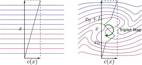
The effect of turbulent stirring is approximated using a mapping function which mimics the effect of a turbulent Eddy on the 1D line. An individual mapping event, known as a triplet map, roughly approximates the effect of a single isotropic Eddy turnover on all the scalars [33, 34]. This is illustrated in Figure 1. An Eddy interval is represented by its lower boundary $x_0$ and its length l. Here, $x_0$ is sampled from a uniform distribution while l follows inertial range scaling laws of three-dimensional turbulence [33, 34]. This can be sampled from the size distribution (11) $f\left(l\right)=\frac{5}{3}\frac{l^{-8/3}}{{\eta }^{-5/3}-{\mathrm{\Delta }}^{-5/3}},$(11) where Δ is the filter width and η is the Kolmogorov scale given by the approximation (12) $\eta =N_{\eta }\frac{\mathrm{\Delta }}{R{e}_{\mathrm{\Delta }}^{3/4}}.$(12) Δ and η bound the range of Eddy sizes. $N_{\eta }$ is an empirical constant which controls the scaling between the Kolmogorov scale and Δ, the LES filter width and is set to 10.76, as in ref. [23]. $R{e}_{\mathrm{\Delta }}$ is the sub-grid turbulent Reynolds number which can be approximated for LES by (13) $R{e}_{\mathrm{\Delta }}=\frac{u^{\prime }\mathrm{\Delta }}{{\nu }_t}.$(13) The sub-grid fluctuating velocity, $u^{\prime }$, and turbulent viscosity, ${\nu }_t$, are obtained from the sub-grid scale (SGS) model. The Eddy frequency per unit domain length (unit: $\left[m^{-1}{s}^{-1}\right]$) is given by (14) $\lambda =\frac{54}{5}\frac{\nu R{e}_{\mathrm{\Delta }}}{C_{\lambda }{\mathrm{\Delta }}^3}\frac{\left[\right(\mathrm{\Delta }/\eta {)}^{5/3}-1]}{[1-(\eta /\mathrm{\Delta }{)}^{4/3}]},$(14) where $C_{\lambda }$ is a modelling constant of value set to 15.0, as in ref. [23]. Note that ν here is the average kinematic viscosity on the LEM line and not the SGS-given ${\nu }_t$ used in Equation (13(13) $R{e}_{\mathrm{\Delta }}=\frac{u^{\prime }\mathrm{\Delta }}{{\nu }_t}.$(13) ). Rearrangement events are assumed to be statistically independent and sampled from a Poisson process where the average time between each event is [33, 34] (15) $\mathrm{\Delta }{t}_{\mathrm{s}\mathrm{t}\mathrm{i}\mathrm{r}\mathrm{r}}=\frac{1}{\lambda L_{\mathrm{L}\mathrm{E}\mathrm{M}}}.$(15) Sub-grid $R{e}_{\mathrm{\Delta }}$ varies spatially over the resolved grid owing to variations of the turbulence intensity. If the filter width Δ is set to the grid spacing and the grid spacing is non-constant, then Δ also varies spatially. Also, $R{e}_{\mathrm{\Delta }}$ is time varying in general, so the quantities specified by Equations (11(11) $f\left(l\right)=\frac{5}{3}\frac{l^{-8/3}}{{\eta }^{-5/3}-{\mathrm{\Delta }}^{-5/3}},$(11) )–(15(15) $\mathrm{\Delta }{t}_{\mathrm{s}\mathrm{t}\mathrm{i}\mathrm{r}\mathrm{r}}=\frac{1}{\lambda L_{\mathrm{L}\mathrm{E}\mathrm{M}}}.$(15) ) are regularly updated for each LEM domain. Mapping/rearrangement events are instantaneous and interrupt the solution of Equations (8(8) $\rho c_p\frac{\mathrm{\partial }T}{\mathrm{\partial }t}=-\frac{\mathrm{\partial }Q}{\mathrm{\partial }x}+S_T,$(8) ) and (9(9) $\rho \frac{\mathrm{\partial }{Y}_{\alpha }}{\mathrm{\partial }t}=-\frac{\mathrm{\partial }{j}_{\alpha ,x}}{\mathrm{\partial }x}+S_{\alpha },$(9) ). Advancement of T and $Y_{\alpha }$ is achieved using a split approach where spatial diffusion is solved using a second order finite difference scheme with implicit time marching while the chemical source terms ($S_T$ and $S_{\alpha }$) are integrated using the Backward Differentiation Formula (BDF) for stiff ODEs. The implicit solver ‘CVODE’ from the SUNDIALS package [35] is used for the latter. Reaction rates and thermodynamic data are handled using the open source software package Cantera [36]. Heat release is assumed to be at constant pressure which necessitates individual LEM cells be allowed to expand to accommodate the density drop due to combustion. This expansion is simply realised as an update to the LEM cell size as (16) $\mathrm{\Delta }{x}_i^{\mathrm{n}\mathrm{e}\mathrm{w}}=\mathrm{\Delta }{x}_i\left(\frac{{\rho }_{i,1}}{{\rho }_{i,\mathrm{n}\mathrm{e}\mathrm{w}}}\right),$(16) where ${\rho }_{i,1}$ and ${\rho }_{i,\mathrm{n}\mathrm{e}\mathrm{w}}$ are the densities of LEM cell i before and after reaction–diffusion advancement, $\mathrm{\Delta }{x}_i$ and $\mathrm{\Delta }{x}_i^{\mathrm{n}\mathrm{e}\mathrm{w}}$ represent widths. Equation (16(16) $\mathrm{\Delta }{x}_i^{\mathrm{n}\mathrm{e}\mathrm{w}}=\mathrm{\Delta }{x}_i\left(\frac{{\rho }_{i,1}}{{\rho }_{i,\mathrm{n}\mathrm{e}\mathrm{w}}}\right),$(16) ) corresponds to a Lagrangian (mass fixed) treatment of individual LEM cells leading to non-uniform LEM cells sizes. Here, we perform a re-gridding after each LEM advancement to enforce a uniform grid-spacing on the LEM line.

Figure 1. Triplet map approximates the stirring effect of a single turnover of an isotropic turbulent Eddy; the coloured lines are concentration isopleths for a scalar; the figure on the left represents a scalar gradient where the straight line shows concentration.

Within a given LES time step $\mathrm{\Delta }{t}_{\mathrm{L}\mathrm{E}\mathrm{S}}$, the mapping/rearrangement events (timings) are sampled from a Poisson process, as mentioned before, with a mean $\mathrm{\Delta }{t}_{\mathrm{s}\mathrm{t}\mathrm{i}\mathrm{r}\mathrm{r}}$. As each (future) Eddy is sampled the LEM line is advanced to that time (after which a new Eddy is sampled) or to elapsed time $\mathrm{\Delta }{t}_{\mathrm{L}\mathrm{E}\mathrm{S}}$, whichever is sooner. Diffusion is advanced between each Eddy event concurrent with advancement of thermochemical source terms. Denoting the diffusion step (between successive mappings or a mapping and elapsed time $\mathrm{\Delta }{t}_{\mathrm{L}\mathrm{E}\mathrm{S}}$) as $\mathrm{\Delta }{t}_{\mathrm{d}\mathrm{i}\mathrm{f}\mathrm{f}}$, the combined diffusion-reaction progress can be split for a formally second order accurate time integration following Strang splitting [37] as $D{D}^{\frac{\mathrm{\Delta }t}{2}}R{R}^{\mathrm{\Delta }t}D{D}^{\frac{\mathrm{\Delta }t}{2}}$, where $DD$ denotes diffusion steps and $RR$ is reaction advancement for $S_T$ and $S_{\alpha }$ (for $\mathrm{\Delta }t=\mathrm{\Delta }{t}_{\mathrm{d}\mathrm{i}\mathrm{f}\mathrm{f}}$).

The routine where triplet map timings are sampled as a Poisson process is termed ‘sampled-sequencing’ in this work. Each Eddy event, as mentioned before, interrupts reaction–diffusion advancement which in turn necessitates re-initialisation of the chemistry solver after each event. Higher frequency of Eddy events leads to more frequent interruptions which leads to slowing-down of the overall code. This is the primary reason why LES–LEM is expensive for high-Reynolds-number cases. Alternatively, the Eddy events for a given LES time step ($=1/\mathrm{\Delta }{t}_{\mathrm{s}\mathrm{t}\mathrm{i}\mathrm{r}\mathrm{r}}$) can be performed (in-sequence) at the beginning of the time step followed by reaction–diffusion advancement for $\mathrm{\Delta }{t}_{\mathrm{L}\mathrm{E}\mathrm{S}}$ i.e. only the position and size of triplet maps are sampled from their respective distributions. This is termed ‘blocked-sequencing’ which reduces the interruptions to the chemistry solver (per CFD time step) which not only improves performance but greatly reduces the dependence of LEM solution time on Reynolds number. For a small enough LES time step, binned statistics generated from blocked-sequencing advancement of LEM should approach that of sampled-sequencing.

2.4. Diffusion fluxes

The diffusion fluxes for temperature Q and the species mass fractions $j_{\alpha }$ are modelled using the gradient model for molecular diffusion i.e. (17) $Q=-\lambda \frac{\mathrm{\partial }T}{\mathrm{\partial }x}$(17) and (18) $j_{\alpha }=-\rho D_{\alpha }\frac{\mathrm{\partial }{Y}_{\alpha }}{\mathrm{\partial }x},$(18) where λ and $D_{\alpha }$ are the thermal conductivity and the (mixture averaged) species diffusion coefficient. Zero-gradient boundary conditions for temperature as well as species mass fractions are used on both ends. Section 2.10 covers wall treatment for wall-adjacent LEM lines in the case of isothermal walls. The reduced dimensionality of LEM allows for affordable computation of differential diffusion using mixture averaged or even binary diffusion coefficients a.k.a. ‘full’ diffusion, which might become relevant for fuels such as hydrogen.

2.5. Cell clustering or ‘super-grid’ setup

The main objective of this work is to reduce the computational expense of LES–LEM. This is achieved by reducing the number of LEM lines in the CFD domain through coarse-graining or agglomeration procedures applied to the CFD/LES level mesh. Each resulting cell-cluster, instead of each CFD cell, then contains a single LEM line responsible for local flame statistics. LEM lines still resolve the flame structure. The speed-up is largely due to a scaling down of the total LEM cell count in the domain, i.e. fewer chemistry advancements per LES time step. If we consider, as an example, a cluster on a cell uniform Cartesian mesh of $10\times 10\times 10={10}^3$ LES cells of resolution $1\mu \mathrm{m}$, each containing a single LEM line of length $1\mu \mathrm{m}$ (of undetermined orientation) and an LEM resolution of $0.1\mu \mathrm{m}$ to resolve flame structures, LES–LEM requires $10\times {10}^3={10}^4$ LEM cells within the cluster, all individually advanced for chemistry. If instead we consider a single LEM line within the entire cluster, only $10\times 10={10}^2$ LEM cells need to be advanced for the same LEM resolution. It is easy to infer that the degree of agglomeration strongly affects this performance improvement. Fewer LEM lines also means fewer splicing operations (and related overheads) per time step, further contributing to a performance improvement over LES–LEM. At this point it is important to note that we are not sacrificing (flame structure) resolution on the LEM line by cell agglomeration.

Modifications are made to the LES advancement to better suit the super-grid configuration. Notably, in Equation (11(11) $f\left(l\right)=\frac{5}{3}\frac{l^{-8/3}}{{\eta }^{-5/3}-{\mathrm{\Delta }}^{-5/3}},$(11) )–(15(15) $\mathrm{\Delta }{t}_{\mathrm{s}\mathrm{t}\mathrm{i}\mathrm{r}\mathrm{r}}=\frac{1}{\lambda L_{\mathrm{L}\mathrm{E}\mathrm{M}}}.$(15) ), Δ is replaced with the cell-cluster integral length scale i.e. (19) $\mathrm{\Delta }:=l_t={\left(\sum _{j\in \mathbf{V}}{V}_j\right)}^{\frac{1}{3}},$(19) where $\mathbf{V}$ is the set of indices of CFD cells that make up the cell cluster and the sum is over cell volumes V. Also, LEM lines have an initial volume equal to that of the respective nominal cell cluster size i.e. that they have a nominal cross-sectional area (20) $A=\frac{\left(\sum _{j\in \mathbf{V}}{V}_j\right)}{l_t}.$(20) Note that the length of the LEM line is variable while its cross sectional area is fixed.

OpenFOAM, by default, uses unstructured meshes which allows an easy discretisation of complex geometries. In order to preserve the benefits of fully unstructured meshes we use the MGridGen [38] routines for CFD cell agglomeration to create the super-grid. Cluster sizes (minimum and maximum) as well as type (in this case ‘globular’) are given as input parameters. The algorithm tries to minimise the summation of (volume-weighted) aspect ratios of all clusters in the domain. Bookkeeping is necessary to record the relationships between the super-grid and CFD mesh e.g. the CFD cells that constitutes a cell-cluster or the CFD faces that form each Super-cell face (face-owner lists). Bookkeeping methods specific to OpenFOAM w.r.t. CFD domain boundaries are given in Appendix.

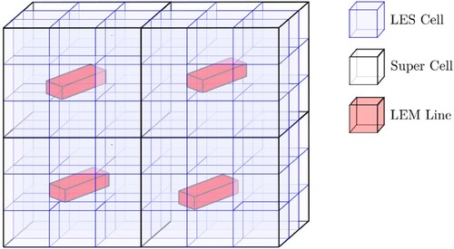
The substantial advantage of SG-LEM in terms of computational cost comes at the price of losing information about the scalar distribution on the LES grid level, so a strategy is needed to recover this information. In the presented strategy, coupling between the LEM and LES level is achieved through PDF weighted integration of conditioned scalars, much like in laminar flamelets or FGM for turbulent combustion modelling. This is explained further in Section 2.7. Figure 2 is a schematic representation of cell-clustered (or super-grid) LES–LEM.

Figure 2. Schematic representation of SG-LEM. LEM line widths are smaller than implied by Equation (20(20) $A=\frac{\left(\sum _{j\in \mathbf{V}}{V}_j\right)}{l_t}.$(20) ).

2.6. Advection between LEM lines

Advection at the CFD level needs to be communicated to the LEM level. This is done through an operation called splicing where LEM fragments are removed from an end of one line and attached to an end of another in a manner that reflects the resolved fluxes between cell clusters. In the current splicing scheme each LEM line has a designated in-splice and out-splice end. This is done to preserve consistent residence times for LEM fragments that have been in-spliced [39]. The splicing routine developed in [13, 39] is employed here, albeit modified for the presented cell-clustering scheme. It has been extended to parallel computation where the CFD domain is decomposed into multiple processor domains. The procedure is as follows:

For a given cell cluster k, let ${\mathbf{O}}_k$ be the set of super-grid faces belonging to the cluster which have a net outward flux and ${\mathbf{I}}_k$ be the set of faces with a net inward flux. Note that flux here refers to volumetric flux with unit [${\mathrm{m}}^3{\mathrm{s}}^{-1}$]. Perform the following steps:

1. Cycle through LEM lines $k\in [1,K]$, where K is the total number of cell clusters (and hence LEM lines) in a given processor domain.

   1. Sort ${\mathbf{O}}_k$ in ascending order of flux $\varphi \left(N\right)$ for $N\in {\mathbf{O}}_k$ where N refers to the face numbers in the (per-processor) cell-cluster numbering scheme; $\varphi \left(N\right)$ is computed as the algebraic sum of CFD-prescribed volume fluxes for the CFD faces that make up cluster face N.

   2. For each N in the sorted list, splice out an LEM fragment of length (21) $L_{N,k}^{frag}=L_k^{\mathrm{L}\mathrm{E}\mathrm{M}}\frac{\varphi \left(N\right)\mathrm{\Delta }{t}_{\mathrm{L}\mathrm{E}\mathrm{S}}}{V_k}$(21) from the designated out-splice end, where $L_k^{\mathrm{L}\mathrm{E}\mathrm{M}}$ is the length of the LEM line and $V_k$ is the volume of the corresponding cell cluster.

   3. For each N, send the fragment to location N of a global fragment list which temporarily holds fragments to be spliced for all faces in a processor domain. Also send the LEM cross-section $A_k$ (c.f. Equation (20(20) $A=\frac{\left(\sum _{j\in \mathbf{V}}{V}_j\right)}{l_t}.$(20) )) to location N of a global cross-section list $\mathbf{A}$.

2. Cycle through LEM lines $k\in [1,K]$

   1. Sort ${\mathbf{I}}_k$ in descending order of flux $\varphi \left(N\right)$ for $N\in {\mathbf{I}}_k$.

   2. For each N in the sorted list:

      1. The LEM fragment stored in the fragment list at location N is modified to account for differences in cross-section and to maintain a consistent 1D representation. The length of each cell i of the fragment is modified as (22) $\mathrm{\Delta }{x}_i^{new}=\mathrm{\Delta }{x}_i\frac{\mathbf{A}\left[N\right]}{A_k},$(22) note that this operation does not affect mass consistency.

      2. Splice in the modified fragment to the designated in-splice end of LEM line k.

The splicing order as dictated by face flux ordering links the current scheme to the concept of control volume crossing rate, i.e. higher fluxes imply higher displacements per time step and vice versa [39]. A key difference between the presented splicing scheme and that which was employed in previous works [12–14, 34] is that LEM fragments are defined by their lengths determined by a volume ratio (step 1c), as opposed to a spliced mass determined by a mass ratio that is computed similarly using resolved mass fluxes. This novel ‘length-based’ scheme allows for splicing between cell clusters of varying cross-sections (step 2(b)i) and hence is pertinent to the super-grid approach presented in this study.

The general scheme outlined above is modified slightly for inflow boundary faces, depending upon whether the case is premixed or non-premixed. For premixed combustion a ‘ghost’ LEM line is initialised with the necessary equivalence ratio for each inflow patch (per-processor). For the latter, fuel and oxidiser inlet patches are each assigned a ghost line initialised, in turn, with fuel and oxidiser stream conditions. From these, LEM fragments are spliced out (step 1b) proportional to fuel and oxidiser fluxes into relevant locations of the fragment list (step 1c). The ghost lines are constantly replenished such that their lengths and resolution remain roughly constant i.e. they remain unaffected by splicing, unlike lines inside the domain.

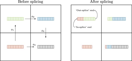
For outflow boundary faces, the fragment list is simply cleared at the required locations. Special care must be taken for splicing across processor boundaries. Here, step 1c is modified where, in addition to sending LEM fragments to the fragment list at processor out-flux locations, LEM fragments from neighbouring processors populate the list at processor in-flux locations, a similar approach is taken for processor cyclic boundaries. The parcel exchanges are handled using the Message Passing Interface (MPI) for distributed memory architectures. The splicing scheme described above allows for the splicing of fractional LEM cells to ensure mass conservation during the process. Figure 3 shows the re-configuration of LEM lines after a flux ordered splicing operation. LEM fragments corresponding to higher fluxes are displaced by larger amounts for a given time step. The reader is directed to ref. [40] for further details on splicing and particularly on the analogy between Lagrangian splicing and Eulerian transport algorithms.

Figure 3. Schematic showing flux ordered splicing; arrows of different length indicate unequal fluxes between cells or cell clusters.

2.7. Coupling with LES

There are several ways to couple the LEM reaction diffusion advancement to LES. One possibility is to compute Favre averaged (density weighted) mean values for temperature and species mass fractions on the line and set these as the sub-grid filtered scalars [32, 34]. This is the standard approach for LES–LEM with an LEM line residing in each LES cell. The filtered quantities along with density from the continuity equation can be used to calculate thermochemical properties, internal energy, enthalpy or iterate $\tilde{T}$ from the enthalpy using the caloric equation of state in each cell of the LES grid. Another is to set source terms for the species transport and energy equations as the LEM averaged production rates [13].

For the cell-clustered variant of LES–LEM, however, there needs to be a way of distributing filtered quantities among the individual LES cells that make up any given cell-cluster. This is achieved using the coupling strategy implemented by Lackmann et al. [16, 23] known as RILEM (Representative Interactive Linear Eddy Model). In RILEM, any thermochemical scalar ψ is conditioned on the LEM line to mixture fraction Z and reaction progress variable c as $〈\psi |Z,c〉$. Here, mixture fraction as defined by Bilger [41] is computed using elemental mass fractions of either $\mathrm{C},\mathrm{H},\mathrm{O},\mathrm{o}\mathrm{r}\mathrm{N}$ relative to the known composition of the fuel stream. The reaction progress variable c is defined as (23) $c=\frac{{\varphi }_{\alpha }-{\varphi }_{\alpha ,\mathrm{u}\mathrm{n}\mathrm{b}\mathrm{u}\mathrm{r}\mathrm{n}\mathrm{t}}}{{\varphi }_{\alpha ,\mathrm{b}\mathrm{u}\mathrm{r}\mathrm{n}\mathrm{t}}-{\varphi }_{\alpha ,\mathrm{u}\mathrm{n}\mathrm{b}\mathrm{u}\mathrm{r}\mathrm{n}\mathrm{t}}},$(23) where ${\varphi }_{\alpha }$ is a choice of thermochemical state variable e.g. T or mass fractions of select species such as ${\mathrm{O}}_2$.

Filtered thermo-chemical scalar values for any LES cell in a cell-cluster are given by weighted integration of corresponding conditioned scalar values with the joint PDF of Z and c, in other words the first moment of the PDF as (24) $\tilde{\psi }(\mathbf{x},t)={\int }_0^1〈\psi |Z,c〉P(Z,c)\mathrm{d}Z\mathrm{d}c.$(24) Assuming statistical independence of Z and c gives (25) $\tilde{\psi }(\mathbf{x},t)={\int }_0^1〈\psi |Z,c〉P\left(Z\right)P\left(c\right)\mathrm{d}Z\mathrm{d}c.$(25) The sub-filter distributions of Z is assumed to follow a β-PDF (written as $P_{\text{β}}(Z;\tilde{Z},\widetilde{Z^{″2}}$)) [23]. Reaction progress and its associated transport equation for the reason progress variable c was incorporated into RILEM in a [16] where it was assumed to follow a Dirac delta-PDF. Alternatively, c can be assumed follow either a double-δ- or β-PDF which was used in this work. For a unique definition of the local PDF shape in each LES cell, transport equations for the Favre mean mixture fraction $\tilde{Z}$ and Favre mean progress variable $\tilde{c}$ are advanced on the CFD side as (26) $\frac{\mathrm{\partial }\left(\overline{\rho }\tilde{Z}\right)}{\mathrm{\partial }t}+\mathrm{\nabla }\cdot \left(\overline{\rho }\tilde{\mathbf{u}}\tilde{Z}\right)=\mathrm{\nabla }\cdot \left[\frac{{\mu }_t}{S{c}_t}\mathrm{\nabla }\tilde{Z}\right]$(26) and (27) $\frac{\mathrm{\partial }\left(\overline{\rho }\tilde{c}\right)}{\mathrm{\partial }t}+\mathrm{\nabla }\cdot \left(\overline{\rho }\tilde{\mathbf{u}}\tilde{c}\right)=\mathrm{\nabla }\cdot \left[\frac{{\mu }_t}{S{c}_t}\mathrm{\nabla }\tilde{c}\right]+\overline{\rho }\tilde{\dot{c}},$(27) where ${\mu }_t$ is the turbulent viscosity, $S{c}_t$ is the turbulent Schmidt number and $\overline{\dot{c}}$ is the source term for Equation (27(27) $\frac{\mathrm{\partial }\left(\overline{\rho }\tilde{c}\right)}{\mathrm{\partial }t}+\mathrm{\nabla }\cdot \left(\overline{\rho }\tilde{\mathbf{u}}\tilde{c}\right)=\mathrm{\nabla }\cdot \left[\frac{{\mu }_t}{S{c}_t}\mathrm{\nabla }\tilde{c}\right]+\overline{\rho }\tilde{\dot{c}},$(27) ) driven by combustion.

2.8. Sub-filter variances

The use of β-PDFs (e.g. $P_{\text{β}}(c;\tilde{c},\widetilde{c^{″2}})$) requires instantaneous variances (here $\widetilde{c^{″2}}$) to be reliably modelled. For RANS-based models this is usually achieved by solving a transport equation for both mixture fraction and progress variable variance (see [23]). For LES, however, algebraic gradient-squared methods are often used [42] for scalar variances. Here $\widetilde{c^{″2}}$ is modelled as (28) $\overline{\rho }\widetilde{c^{″2}}=C_v{\mathrm{\Delta }}^2\overline{\rho }{\left|\mathrm{\nabla }\tilde{c}\right|}^2,$(28) where $C_v$ is a model coefficient. A similar approach can be used for $\widetilde{Z^{″2}}$. For the current implementation a constant value of 1/12 is used for simplicity. The derivation for and performance of this approach can be found in ref. [42] where it is termed SCF (static coefficient model).

2.9. Scalar conditioning

Conditioning a scalar ψ as $〈\psi |Z,c〉$ at the LEM level practically involves dividing the range of Z and c into discrete bins. Let $Z\left(j\right)$ and $c\left(k\right)$ denote the discrete values defining the boundaries between bins in $(Z,c)$-space. Then bin $(Z_j,c_k)$ covers the range $Z\left(j\right)\le Z<Z(j+1)$ and $c\left(k\right)\le c<c(k+1)$. The value of scalar ψ conditioned to $(Z_j,c_k)$ is found using conventional averaging as (29) $〈\psi |Z_j,c_k〉=\frac{\sum _{i\in \mathcal{B}}{\psi }_i}{|\mathcal{B}|},$(29) where $\mathcal{B}$ is the set of LEM cells which satisfies $Z\left(j\right)\le Z<Z(j+1)$ and $c\left(k\right)\le c<c(k+1)$ and $|\mathcal{B}|$ is the number of elements in $\mathcal{B}$. Density weighted conditioning can be implemented as (30) $〈\psi |Z_j,c_k〉=\frac{\sum _{i\in \mathcal{B}}{\psi }_i{\rho }_i}{\sum _{i\in B}{\rho }_i}.$(30) Filling every bin from a single LEM line at a given time is unlikely due to the relatively small number of cells along each LEM line and the fact that each LEM line is just a snapshot of the current state. This leads to bins without values, called ‘holes’. However, for the evaluation of the PDF integrals in (25(25) $\tilde{\psi }(\mathbf{x},t)={\int }_0^1〈\psi |Z,c〉P\left(Z\right)P\left(c\right)\mathrm{d}Z\mathrm{d}c.$(25) ) a completely filled state in Z, c-space is required. This is achieved by persisting values in each bin until LEM cells with suitable c values are encountered. Additionally, $〈\psi |Z_j,c_k〉$ must be initialised, prior to conditioning, with either unburnt values or the data from a zero-dimensional reactor. Persistence is applied to each scalar individually. There is also the choice to have them reset to their initial values, after each conditioning event, in order to capture extinction or re-ignition effects, but this would incur a reduction in fidelity.

The first moment also yields the source term for Equation (27(27) $\frac{\mathrm{\partial }\left(\overline{\rho }\tilde{c}\right)}{\mathrm{\partial }t}+\mathrm{\nabla }\cdot \left(\overline{\rho }\tilde{\mathbf{u}}\tilde{c}\right)=\mathrm{\nabla }\cdot \left[\frac{{\mu }_t}{S{c}_t}\mathrm{\nabla }\tilde{c}\right]+\overline{\rho }\tilde{\dot{c}},$(27) ): (31) $\overline{\dot{c}}(\mathbf{x},t)={\int }_0^1〈\dot{c}|Z,c〉P(Z;\tilde{Z},\widetilde{Z^{″2}})P(c;\tilde{c},\widetilde{c^{″2}})\mathrm{d}Z\mathrm{d}c,$(31) where $\dot{c}$ at the LEM level is given by the time derivative of (23(23) $c=\frac{{\varphi }_{\alpha }-{\varphi }_{\alpha ,\mathrm{u}\mathrm{n}\mathrm{b}\mathrm{u}\mathrm{r}\mathrm{n}\mathrm{t}}}{{\varphi }_{\alpha ,\mathrm{b}\mathrm{u}\mathrm{r}\mathrm{n}\mathrm{t}}-{\varphi }_{\alpha ,\mathrm{u}\mathrm{n}\mathrm{b}\mathrm{u}\mathrm{r}\mathrm{n}\mathrm{t}}},$(23) ): (32) $\dot{c}=\frac{1}{{\varphi }_{\alpha ,\mathrm{b}\mathrm{u}\mathrm{r}\mathrm{n}\mathrm{t}}-{\varphi }_{\alpha ,\mathrm{u}\mathrm{n}\mathrm{b}\mathrm{u}\mathrm{r}\mathrm{n}\mathrm{t}}}\frac{\mathrm{d}{\varphi }_{\alpha }}{\mathrm{d}t}.$(32) Note that formulation with Z and c is shown here for generality but can be reduced for premixed flames by omitting Z as a conditioning variable, effectively reducing $〈\psi |Z,c〉$ to $〈\psi |c〉$ and setting $P\left(Z\right)=1.0$ in Equation (25(25) $\tilde{\psi }(\mathbf{x},t)={\int }_0^1〈\psi |Z,c〉P\left(Z\right)P\left(c\right)\mathrm{d}Z\mathrm{d}c.$(25) ). This also eliminates the need for Equation (26(26) $\frac{\mathrm{\partial }\left(\overline{\rho }\tilde{Z}\right)}{\mathrm{\partial }t}+\mathrm{\nabla }\cdot \left(\overline{\rho }\tilde{\mathbf{u}}\tilde{Z}\right)=\mathrm{\nabla }\cdot \left[\frac{{\mu }_t}{S{c}_t}\mathrm{\nabla }\tilde{Z}\right]$(26) ). This reduced version is used for the premixed test case presented in section 3. Similarly, non-premixed flames using the fast chemistry assumption can be approached by omitting c and Equation (27(27) $\frac{\mathrm{\partial }\left(\overline{\rho }\tilde{c}\right)}{\mathrm{\partial }t}+\mathrm{\nabla }\cdot \left(\overline{\rho }\tilde{\mathbf{u}}\tilde{c}\right)=\mathrm{\nabla }\cdot \left[\frac{{\mu }_t}{S{c}_t}\mathrm{\nabla }\tilde{c}\right]+\overline{\rho }\tilde{\dot{c}},$(2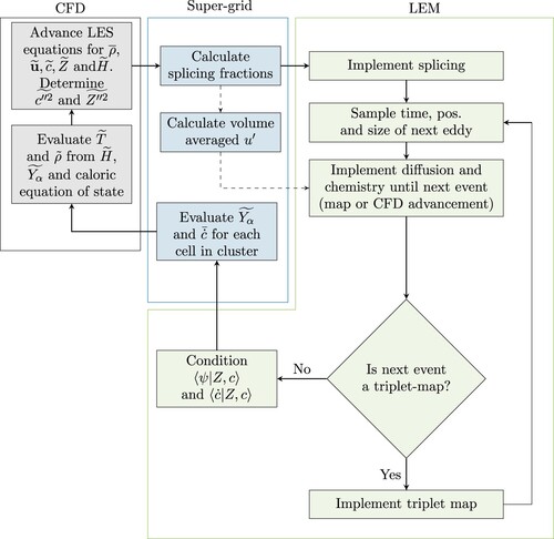7) ). Figure 4 shows the interface between the LEM, super-grid and flow solver levels.

Figure 4. Interface between LES, super-grid and LEM.

2.10. Wall treatment

Modelling of near wall effects can be necessary for accurate flame structure and radical predictions. LEM, by its very formulation, can only handle gaseous reacting mixtures. This necessitates transfer functions which convey heat and mass information from sources such sprays or walls to the LEM level, if these features are present in the CFD domain [23]. For the case of an isothermal wall, considered in the test case below, a straightforward wall treatment is obtained by identifying cell-clusters (and therefore LEM lines) that are adjacent to the walls and attaching one end of those LEM lines to the wall patch i.e. we effectively impose wall temperature as a Dirichlet boundary condition to one end of the LEM line as it pertains to temperature diffusion advancement. Splicing (both in- and out-splicing) are now performed exclusively at the remaining free end. Finally, LES-resolved temperatures depend on the enthalpy transport (5(5) $\frac{\mathrm{\partial }\left(\overline{\rho }\tilde{H}\right)}{\mathrm{\partial }t}+\frac{\mathrm{\partial }\overline{\rho }{\tilde{u}}_j\tilde{H}}{\mathrm{\partial }{x}_j}={\tilde{u}}_j\frac{\mathrm{\partial }\overline{p}}{\mathrm{\partial }{x}_j}+\frac{\mathrm{\partial }}{\mathrm{\partial }{x}_j}\left({\alpha }_{\mathrm{E}\mathrm{f}\mathrm{f}}\frac{\mathrm{\partial }\tilde{H}}{\mathrm{\partial }{x}_j}\right)+\frac{\mathrm{\partial }p}{\mathrm{\partial }t}.$(5) ) for which the Eddy-diffusivity treatment is applied to wall as well as non-wall LES-cell faces.

3. Test case and numerical setup

Validation for the proposed method was performed against a reactive DNS for a premixed ethylene flame in a backward-facing-step configuration show in ref. [27]. While a reduced mechanism consisting of 22 species [43] was used in the DNS solution, a 32 species skeletal mechanism from the same reference was used here for the SG-LEM simulations.¹ The computational domain is shown in Figure 5(a). The LES mesh was created using a multi-block approach and consists of hexagonal cells.

Figure 5. Numerical setup for the test case. (a) The computational domain. $H=1.466\mathrm{c}\mathrm{m}$ and $D=0.3048\mathrm{c}\mathrm{m}$, spanwise width is $1\mathrm{c}\mathrm{m}$ and (b) LES mesh.

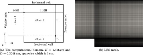
An ethylene-air mixture, with equivalence ratio 0.42 and temperature 1125 K, is introduced into the domain with an inlet bulk velocity of $200\mathrm{m}{\mathrm{s}}^{-1}$. This corresponds to a Mach number of 0.3 which justifies the use of a pressure based solver. We do not expect to see shocks or other compressibility-driven flow features in the domain which would require the use of a density based solver instead. An a priori (non-reacting) simulation with the appropriate channel cross-section was used to generate fully developed channel flow for the inlet. The mean velocity profile from this precursor simulation was augmented with synthetic turbulence imposed at the inlet.² The inlet temperature profile was prescribed using a power-law function (in y) which was curve-fit to the time averaged inlet temperature in the DNS data. A non-reflecting pressure outlet mitigates pressure waves that reflect back and forth between the isothermal walls, which are at 600 K.

Periodic boundaries are applied to the spanwise direction while ambient pressure was set to 1.72 atm. The mesh has a uniform cell size of 0.01 cm in all directions but with an expansion ratio of 10 applied to the wall normal direction, which lead to around 6.2 M cells. Pressure-velocity coupling is achieved using the PISO (Pressure-implicit with splitting of operators) methodology [44] using 2 pressure corrector loops per CFD time advancement. The cluster size was set to 125 while LEM resolution was set to $26\mu \mathrm{m}$, comparable to the cell sizes used in the DNS study. Also tested was a cluster size of 1000 to assess performance and sensitivity (see Section 4.4).

Conditioned values $〈\psi |c〉$ were initialised using a zero-dimensional reactor in which the fuel-air mixture was advanced until equilibrium. Simultaneously, mass fractions and $\dot{c}$ were conditionally averaged into 100 discrete bins in c-space to initialise $〈\psi |c〉$ for all LEM lines. The reader is reminded that the reduced RILEM formulation using only c is used for this premixed test case. Here, $Y_{{\mathrm{O}}_2}$ is used for calculating c at the LEM level, in accordance with the DNS simulation and, importantly, β-PDFs were assumed for sub-filter c where $\widetilde{c^{″2}}$ is modelled using Equation (28(28) $\overline{\rho }\widetilde{c^{″2}}=C_v{\mathrm{\Delta }}^2\overline{\rho }{\left|\mathrm{\nabla }\tilde{c}\right|}^2,$(28) ). Persistence was applied to mass fractions, production rates as well as $\dot{c}$ at the LEM level. The SG-LEM solver was run for 20 flow-through times ($\approx 20\times {10}^{-4}\mathrm{s}$) to get a statistically stationary flame. The Smagorinsky SGS model [29] was used to close the momentum equation. Time averaging of scalars began after 15 flow passes. All simulations were performed on the HPC cluster Vera from the Swedish National Infrastructure for Computing (SNIC), running Intel Xeon Gold 6130 CPUs.

4. Results and discussion

The proposed SG-LEM is a new approach to simulate turbulent combustion. In the following we will therefore address some fundamental questions and qualitative features of SG-LEM and also compare results with the available DNS data. In particular, we will address the following points:

1. The ability of the RILEM-closure using presumed PDFs (here, β PDFs for c) to produce LES-resolved flame structures.

2. Comparison with time averaged DNS data.

3. The impact of clustering parameters, particularly that of cluster size.

4. Computational performance and comparison with traditional LES–LEM.

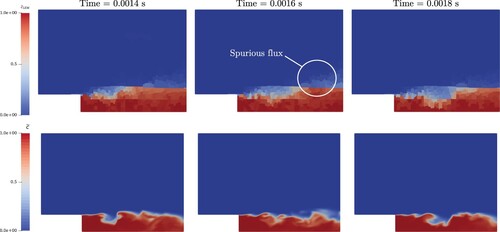
4.1. Qualitative flame structure resolution

This modelling approach for simulating turbulent premixed combustion relies on a physically sound evolution of the reaction progress variable Equation (27(27) $\frac{\mathrm{\partial }\left(\overline{\rho }\tilde{c}\right)}{\mathrm{\partial }t}+\mathrm{\nabla }\cdot \left(\overline{\rho }\tilde{\mathbf{u}}\tilde{c}\right)=\mathrm{\nabla }\cdot \left[\frac{{\mu }_t}{S{c}_t}\mathrm{\nabla }\tilde{c}\right]+\overline{\rho }\tilde{\dot{c}},$(27) ), which, primarily depends on the evaluation of the source term $\tilde{\dot{c}}$. 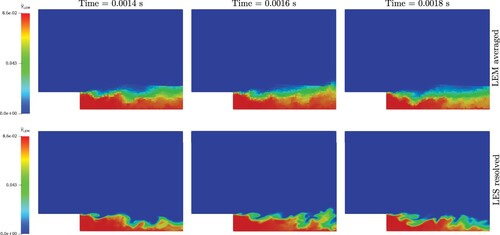The source term itself, according to Equation (25(25) $\tilde{\psi }(\mathbf{x},t)={\int }_0^1〈\psi |Z,c〉P\left(Z\right)P\left(c\right)\mathrm{d}Z\mathrm{d}c.$(25) ), depends on both the LEM solution available at super-grid resolution (providing conditioned scalar values) and the LES solution (providing LES resolved shapes of the PDF). Figure 6 shows snapshots of the LEM averaged Favre mean progress variable reported at the super-grid level and the progress variable Favre mean as advanced by Equation (27(27) $\frac{\mathrm{\partial }\left(\overline{\rho }\tilde{c}\right)}{\mathrm{\partial }t}+\mathrm{\nabla }\cdot \left(\overline{\rho }\tilde{\mathbf{u}}\tilde{c}\right)=\mathrm{\nabla }\cdot \left[\frac{{\mu }_t}{S{c}_t}\mathrm{\nabla }\tilde{c}\right]+\overline{\rho }\tilde{\dot{c}},$(27) ), i.e. at the LES level. Of note is that the top row in Figure 6 evolves purely from LEM advancement combined with splicing, which is driven by fluxes resolved at the super-grid level. The splicing methodology is able to capture the overall flame structure (here, in terms of reaction progress) and retains the recirculation stabilised nature of the setup even after several flow passes. Additionally, due to the high inlet velocity of the reactant mixture, the flame does not propagate upwards and remains nearly horizontal. This indicates that the super-grid approach has a strong potential to provide locally relevant flame statistics. The similarity in the resolved structures between the left and bottom row is encouraging and also supports the source term given by Equation (31(31) $\overline{\dot{c}}(\mathbf{x},t)={\int }_0^1〈\dot{c}|Z,c〉P(Z;\tilde{Z},\widetilde{Z^{″2}})P(c;\tilde{c},\widetilde{c^{″2}})\mathrm{d}Z\mathrm{d}c,$(31) ) as being able to resolve a much finer flame structure than the super-grid on which $\dot{c}$ is conditioned. There are visible differences since the distribution of reactants and burnt products at the LEM level are highly subject to numerical dissipation of super-grid-resolved fluxes (by way of splicing) whereas a transport equation such as (27(27) $\frac{\mathrm{\partial }\left(\overline{\rho }\tilde{c}\right)}{\mathrm{\partial }t}+\mathrm{\nabla }\cdot \left(\overline{\rho }\tilde{\mathbf{u}}\tilde{c}\right)=\mathrm{\nabla }\cdot \left[\frac{{\mu }_t}{S{c}_t}\mathrm{\nabla }\tilde{c}\right]+\overline{\rho }\tilde{\dot{c}},$(27) ) is evolved at LES-resolution. Therefore, super-grid resolution, or specifically the coarse-graining limit, is a parameter of interest in SG-LEM (c.f. Section 4.4).

Figure 6. Top row: snapshots of Favre averaged progress variable c at the LEM level; bottom row: LES resolved $\tilde{c}$ as advanced by Equation (27(27) $\frac{\mathrm{\partial }\left(\overline{\rho }\tilde{c}\right)}{\mathrm{\partial }t}+\mathrm{\nabla }\cdot \left(\overline{\rho }\tilde{\mathbf{u}}\tilde{c}\right)=\mathrm{\nabla }\cdot \left[\frac{{\mu }_t}{S{c}_t}\mathrm{\nabla }\tilde{c}\right]+\overline{\rho }\tilde{\dot{c}},$(27) ) at different times; scalars imaged at $z=0.5\mathrm{c}\mathrm{m}$; 125 CFD cells per cluster.

4.2. Instantaneous mapping closure results

Figure 7 shows temperature snapshots. In SG-LEM there are different ways to report temperature i.e. LEM-averaged temperatures (row I) at the super-grid resolution, temperature iterated from the LES resolved total enthalpy using the caloric equation of state (row II), and PDF weighted integrated temperatures (row III) which reflects binned temperature statistics from the LEM lines. The coarser resolution of the super-grid averaged LEM solution is clearly visible in row I. Note that these are purely the result of LEM advancement and splicing which is driven by super-grid resolved fluxes. The integrated temperatures (row III) show slight artefacts in the form of blocky structures that belie the coarse mesh and the effects of the applied wall treatment. Note that row II temperatures are used to compute density for the flow solver while row III is additional information for diagnosis. Mapped ${\mathrm{C}\mathrm{O}}_2$ mass fractions in Figure 8 suggests that RILEM closure using β PDFs (c.f. Equation (24(24) $\tilde{\psi }(\mathbf{x},t)={\int }_0^1〈\psi |Z,c〉P(Z,c)\mathrm{d}Z\mathrm{d}c.$(24) )) could work well for major species, evidenced by the lack of mapping artefacts and the agreement between the LEM and LES ranges.

Figure 7. Row I: snapshots of Favre averaged T the LEM level; row II: LES resolved $\tilde{T}$ as advanced by Equation (5(5) $\frac{\mathrm{\partial }\left(\overline{\rho }\tilde{H}\right)}{\mathrm{\partial }t}+\frac{\mathrm{\partial }\overline{\rho }{\tilde{u}}_j\tilde{H}}{\mathrm{\partial }{x}_j}={\tilde{u}}_j\frac{\mathrm{\partial }\overline{p}}{\mathrm{\partial }{x}_j}+\frac{\mathrm{\partial }}{\mathrm{\partial }{x}_j}\left({\alpha }_{\mathrm{E}\mathrm{f}\mathrm{f}}\frac{\mathrm{\partial }\tilde{H}}{\mathrm{\partial }{x}_j}\right)+\frac{\mathrm{\partial }p}{\mathrm{\partial }t}.$(5) ) along with (7(7) $\tilde{H}=\sum _{\alpha =1}^N{\tilde{Y}}_{\alpha }\times \left(h_{\alpha }\right(T)+h_{\alpha }^0),$(7) ); row III: LES resolved $\tilde{T}$ as advanced by Equation (25(25) $\tilde{\psi }(\mathbf{x},t)={\int }_0^1〈\psi |Z,c〉P\left(Z\right)P\left(c\right)\mathrm{d}Z\mathrm{d}c.$(25) ) for corresponding times (units [K]). Scalars imaged at $z=0.5\mathrm{c}\mathrm{m}$.

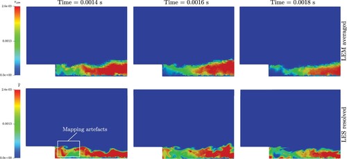
Figure 8. Top row: snapshots of Favre averaged $Y_{{\mathrm{C}\mathrm{O}}_2}$ at the LEM level; bottom row: LES resolved ${\tilde{Y}}_{{\mathrm{C}\mathrm{O}}_2}$ as advanced by Equation (25(25) $\tilde{\psi }(\mathbf{x},t)={\int }_0^1〈\psi |Z,c〉P\left(Z\right)P\left(c\right)\mathrm{d}Z\mathrm{d}c.$(25) ) for corresponding times. Scalars imaged at $z=0.5\mathrm{c}\mathrm{m}$.

RILEM-closure for radical OH is shown in Figure 9. Some mapping artefacts can be seen the zoomed-in region with areas of mass fraction higher than the LEM levels (see range of colour bars), and blocky structures similar to Figure 7 (row III). The latter artefact is not unexpected as the binned statistics for radical species can vary sharply between neighbouring clusters as opposed to the more smoothly varied statistics for ${\mathrm{C}\mathrm{O}}_2$. The former could stem from a combination of the sensitive nature of the β-PDF, especially as $\tilde{c}\to 0\mathrm{o}\mathrm{r}1$, and the initialisation of $〈\psi |c〉$ using the zero-dimensional reactor.

Figure 9. Top row: Favre averaged $\mathrm{O}\mathrm{H}$ mass fractions for each LEM line; bottom row: LES resolved $\mathrm{O}\mathrm{H}$ mass fractions using Equation (25(25) $\tilde{\psi }(\mathbf{x},t)={\int }_0^1〈\psi |Z,c〉P\left(Z\right)P\left(c\right)\mathrm{d}Z\mathrm{d}c.$(25) ).

4.3. Comparison with DNS data

Here we compare the thermochemical results for the test case with time-averaged DNS data. Also shown are results from an LES-PaSR simulation (using an identical setup) using the standard reactingFoam solver from OpenFOAM. As mentioned before, data for time averaging was gathered after 15 flow-through times ($\approx 15\times {10}^{-4}\mathrm{s}$), to minimise the effect of initial transients, and gathered for 5 flow-through times. Additionally, data was averaged in the spanwise z direction. The line plots shown in Figures 10 through 13 show this averaged data along the ( normalised) wall-normal direction at different streamwise locations.

Figure 10. Mean velocity $U_x$ profiles.

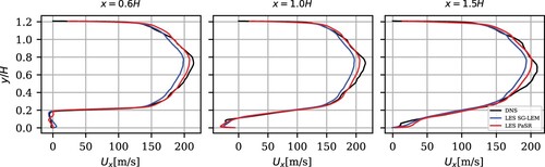
Velocity plots in Figure 10 show that the solution given by the LES setup can accurately capture the mean flow features of the test case. This setup includes the mesh, choice of SGS model and treatment of inlet flow conditions. A part of the recirculation zone is shown by negative velocities at x = H.

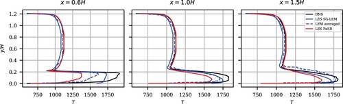
Mean temperature plots in Figure 11 indicates lower temperature development near the step for both SG-LEM and PaSR, as compared to DNS. This is true for both the LEM-averaged and iterated temperature, marked as ‘LES SG-LEM’ in the legend. Temperatures reach better agreement downstream. LEM temperatures driven by splicing at this cluster size show that the super-grid resolved flame remains mostly horizontal, with some slight upward deflection at x = 1.5H. Overall, SG-LEM gives better mean temperatures than PaSR for this setup. Near wall temperatures show that the wall-treatment described in Section 2.10 is performing well.

Figure 11. Mean temperature profiles.

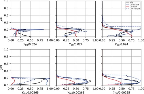
Normalised mean mass fractions for ${\mathrm{C}\mathrm{O}}_2$, ${\mathrm{H}}_2\mathrm{O}$, CO and OH are shown in Figure 12. The lower mean temperatures near the step given by could be explained by the under-prediction in ${\mathrm{H}}_2\mathrm{O}$, this to common to both SG-LEM and PaSR. As with temperature, better agreement can be seen downstream for ${\mathrm{C}\mathrm{O}}_2$ and ${\mathrm{H}}_2\mathrm{O}$ with SG-LEM and PaSR reporting similar values. The more challenging diagnostics, i.e. radicals CO and OH, demonstrate the better predictive capability of SG-LEM, which is exactly the point of using LEM in general. SG-LEM over-predicts peak CO values but, unlike PaSR, correctly predicts the downstream location of the peak as being near the shear layer as opposed to the near-wall region. The OH profile near the step shows the β-PDF integrated mass fractions are markedly different from the Favre averaged mass fractions reported at the coarse level, but this is not the case for the other species. These differences can arise from both the initialisation of the conditioned scalars and the conditioning procedure itself (c.f. Section 2.9 and Figure 9) when applied to an intermediate specie. Downstream OH values are in good agreement with DNS data while PaSR values are underpredicted.

Figure 12. Mean mass fractions.

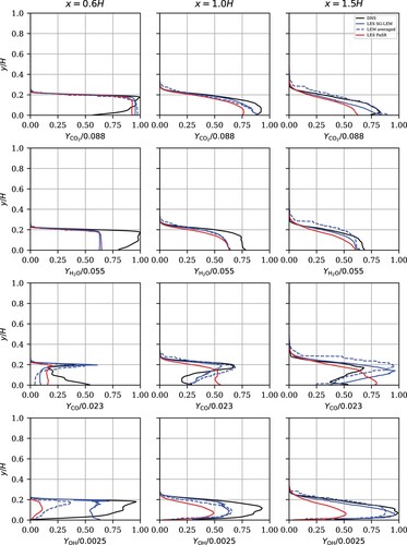
Figure 13 presents scaled reaction rates. Although the LES-resolved values (blue lines) are not used for the mapping-type closure, they are included here as they reveal important features of SG-LEM. Notably, they exhibit a significant resemblance to the DNS data, particularly downstream of the step. The blue dashed lines represent the species production averaged over each LEM line. The disparity between these values and the LES-resolved ones suggests variations in the PDFs of c at the LEM and LES levels. From this perspective, LES-resolved PDFs are more physical as they reflect the advective fluxes of $\tilde{c}$ within each cell cluster, thereby reflecting the resolved flow physics. This serves to illustrate how LEM and LES complement each other by combining detailed TCI with well-resolved advective transport in physical space, resulting in a high level of fidelity. Note that c-conditioned production rates were initialised to zero, hence the LES values in Figure 13 purely reflect on-the-fly statistics.

4.4. Super-grid resolution and numerical dissipation

Given that the fluxes for LEM splicing are resolved at the super-grid level, it is logical to assume a coarse resolution could result in an inaccurate distribution of the fuel-air mixture as well as burnt products in the domain. Figure 14 shows snapshots of $\tilde{c}$ in the same manner as Figure 6, but for cluster size of 1000. This corresponds to 10 cells in each direction for a Cartesian mesh however it should be noted that MGridGen does not always give perfectly ‘globular’ cell-clusters. Cluster shapes are heavily influenced by the overall shape of the processor domain and impact numerical dissipation, as do cluster sizes.

Figure 13. Species reaction rates, scaled [$\mathrm{k}\mathrm{m}\mathrm{o}\mathrm{l}{\mathrm{m}}^{-3}{\mathrm{s}}^{-1}$].

Figure 14. Top row: snapshots of Favre averaged c at the LEM level; bottom row: LES resolved $\tilde{c}$ for corresponding times. Scalars imaged at $z=0.5\mathrm{c}\mathrm{m}$. 1000 CFD cells per cluster.

Despite the differences in super-grid distribution of progress variable, the overall flame structure w.r.t. the $\tilde{c}$ transport Equation (27(27) $\frac{\mathrm{\partial }\left(\overline{\rho }\tilde{c}\right)}{\mathrm{\partial }t}+\mathrm{\nabla }\cdot \left(\overline{\rho }\tilde{\mathbf{u}}\tilde{c}\right)=\mathrm{\nabla }\cdot \left[\frac{{\mu }_t}{S{c}_t}\mathrm{\nabla }\tilde{c}\right]+\overline{\rho }\tilde{\dot{c}},$(27) ) remains qualitatively unchanged (c.f. Figure 6). This suggests a degree of robustness in the approach to $\tilde{c}$ advancement. The CFD-level advancement of mean reaction progress compensates for the poor flux resolution by the super-grid, as demonstrated in Figure 15. The mean profiles for $\tilde{c}$ exhibit similar characteristics for both cluster sizes, even though the LEM level data shows a greater displacement of burnt products (towards the downstream) into the bulk flow for the coarser super-grid.

Figure 15. Mean c profiles, comparing cluster sizes of 125 and 1000.

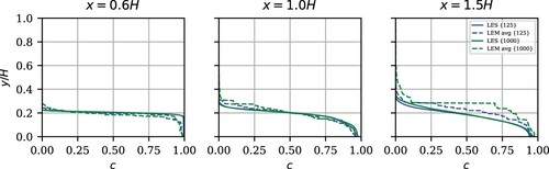
Overall, these findings highlight the ability of the SG-LEM approach to maintain the overall flame structure and robustness in advancing the mean progress variable, despite potential limitations in super-grid flux resolution. Conversely, the improved statistical fidelity for conditioned data, due to having more LEM-cells per cluster, leads to a notable improvement in LES-resolved mass fractions for radicals, as demonstrated in Figure 16. Mean profiles for (LES-resolved) temperature, velocity and major species are nearly identical to what was achieved using a cluster size of 125 and so are omitted here.

Figure 16. Mean profiles for radical mass fractions, cluster size of 1000.

4.5. Computational requirements

Table 1 presents the compute-times for the simulations used in this analysis. The reduction seen between SG-LEM125 and SG-LEM1000 can be primarily attributed to a decrease in LEM advancement times, with minimal improvements in splicing overheads. Overheads associated with RILEM-closure are approximately the same as β-PDFs are generated on-the-fly for each LES cell. Still, SG-LEM125 outperforms PaSR in terms of speed as it eliminates the need to advance transport equations for individual species and instead has employs single mean progress variable.

Table 1. Performance comparison.

#	Combustion closure	Time (h)
1	PaSR	108
2	SG-LEM125	50
3	SG-LEM1000	40
4	LES–LEM	969 (estimated)

Note: Numbers in curly brackets indicate number of CFD cells per cell-cluster.All simulations used a grid size of 6.2 M cells and 256 processors.

Due to resource constraints, performing a full simulation using standard LES–LEM with the current setup and mechanism was found to be infeasible. Nonetheless, we estimate the time requirement for an LES–LEM solution by advancing an LES–LEM solver for a few time-steps to record the LEM advancement times. For a direct comparison, the LEM cell size was set to $26\mu \mathrm{m}$. We recorded a normalised LEM time (relative to SG-LEM125 LEM advancement) of approximately 26.74, while LEM splicing accounted for 1.84. This highlights how splicing constitutes a significant computational expense for standard LES–LEM. Based on these observations, and assuming similar flow-advancement and temperature iteration times, we estimate by simple linear scaling that standard LES–LEM would require approximately 960 hours on the same hardware. This clearly demonstrates the reduction of LEM advancement achieved through the coarse-graining operation, which is one of the primary objectives of SG-LEM.

5. Conclusion and future work

In this study we present a novel mapping-type closure for LES using LEM. Our method, called super-grid LES–LEM (SG-LEM), introduces coarse-graining procedures on the CFD mesh which enable significant computational speed-up compared to standard LES–LEM approaches.

SG-LEM utilises presumed PDFs, akin to flamelet models, to couple the LES and LEM solution domains. It inherits desirable features of LEM i.e. highly resolved flame structures, straightforward diffusion computation and direct implementation of turbulent advection. Additionally, we introduce a ‘length-based’ splicing procedure pertinent to the new coarse-grained formulation. The method produces high-resolution flame structures that strongly influence the flow solution, while also enabling the reporting of chemistry output at the coarse mesh level.

The adopted coupling strategy, called ‘RILEM-closure’, uses presumed β-PDFs to produce good LES-resolved fields for major species and temperature. Although instantaneous mapping artefacts could be seen for radical OH, they do not significantly impact the overall predictive capability of SG-LEM. LEM is capable of capturing transient phenomena like extinction and re-ignition; it remains unclear, however, if RILEM-closure can communicate this information to the LES level within the required time scales. For statistically stationary flames, though, this is likely not a concern.

To validate SG-LEM, we compare simulation results with time-averaged DNS data for a premixed backward facing step configuration. Findings indicate temperature, species mass fractions and reaction rates are in good agreement for downstream locations, with some inaccuracies immediately behind the step. Results also support the treatment applied to wall-adjacent LEM cells, at least for this case involving isothermal walls. Overall, SG-LEM demonstrates better predictive capability than PaSR for intermediate species while requiring approximately half the compute-time on identical hardware, when utilising a cluster size of 125.

The new approach shows tremendous speed-up when compared to traditional LES–LEM and even competes favourably with standard models like PaSR, as demonstrated in our tests. Further speed improvements could be achieved by employing larger clusters; however, we observe some sensitivity to this parameter due to super-grid resolved fluxes that determine splicing. Cases with complex flow features may require smaller cell-clusters to capture important flow features, while simpler cases could benefit from the improved computation offered by larger (and fewer) cell clusters, as well as increased statistical fidelity for conditioned data as shown in our tests. Nonetheless, employing very coarse super-grids may not provide proportionate performance improvements when using on-the-fly β-PDF generation.

We anticipate that future implementations of a solution-adaptive super-grid approach could further enhance the predictive capabilities SG-LEM while reducing computational cost compared to the approach presented in this study.

The use of β functions for the sub-grid distribution of progress variable required a reliable variance model for the same. A simple algebraic model for LES was used in this study but more sophisticated approaches, such as the dynamic procedure outlined by Pierce and Moin [45], could be explored in future work. Furthermore, studies will also examine other flow configurations and combustion regimes to broaden the assessment of SG-LEM. Nevertheless, SG-LEM is capable of providing high fidelity reaction-rate statistics at low computational costs, representing a marked improvement over standard LES–LEM closure.

Acknowledgements

The authors would like to acknowledge the Swedish National Infrastructure for Computing (SNIC) at the Chalmers Centre for Computational Science and Engineering (C3SE) for providing the computational and storage resources needed for this work via projects SNIC 2019/3-181, 2020/6-187, 2020/5-200 and 2022/23-413.

The authors are grateful to Konduri Aditya, Indian Institute for Science (IISc), and Jacqueline Chen, Sandia National Laboratories, for providing the DNS data used for the method validation.

Disclosure statement

No potential conflict of interest was reported by the author(s).

Additional information

Funding

It was partially funded by the Swedish Research Council through grant agreement no. 2018-05973.

Notes

1 Mechanism reduction is realised through a run-time subroutine in the CHEMKIN environment, a feature which is not implemented with Cantera used in this project. Hence, the skeletal mechanism which formed the basis for the reduced one (used in the DNS study) was used here.

2 A pseudo random number generator is used to add between ±5% of the mean velocity (in each direction) during run-time to create synthetic turbulence. Even though the resulting velocity field is not strictly divergence free at the inlet, the pressure corrector loop shortly creates physically meaningful values.

Appendix. SG-LEM bookkeeping for OpenFOAM

In OpenFOAM terminology, a ‘patch’ is defined as one or more enclosed areas of the boundary surface which may or may not be proximal. MGridGen does not coarsen boundaries and in general does not account for boundary patches such as inlets, outlets or walls. For the described splicing method (Section 2.6) this must be addressed. Super-grid boundary faces for a given boundary patch, per processor, are created by agglomeration. The procedure involves scanning the CFD faces comprising the given patch and collecting those CFD faces owned by the same cell-cluster(s) into individual coarse mesh boundary face(s). This results in as many coarse boundary faces as the number of cell-clusters adjacent to a given patch. The procedure is slightly altered for processor boundary patches. Since MGridGen works independently in each processor domain, it is unlikely that cell-clusters have contiguous boundary-normal faces across processor boundaries i.e. neighbouring processor domains could end up with inconsistent super-grid boundary faces w.r.t the CFD cells that comprise them. This must also be addressed for correct splicing. The following procedure ensures consistency for a given processor patch:

1. Scan through the CFD faces i that comprise this processor patch. Let the cell-cluster owner of i be $So\left[i\right]$ and corresponding owner on the neighbouring processor be $Nb\left[i\right]$.

2. Collect i into set $\mathbf{F}$ until $\left(So\right[i+1]\ne So[i\left]\right)\vee \left(Nb\right[i+1]\ne Nb[i\left]\right)$.

3. Designate $\mathbf{F}$ as a new coarse boundary face.

4. Repeat steps 2 and 3 until all faces for the patch have been assigned to a coarse mesh face.

The resulting face numbering scheme is arrived at independently by both domains on either side of the processor patch, but are consistent nonetheless.

References

- J. Janicka and A. Sadiki, Large Eddy simulation of turbulent combustion systems, Proc. Combust. Inst. 30 (2005), pp. 537–547. Available at https://doi.org/10.1016/j.proci.2004.08.279.
- H. Pitsch, Large-Eddy simulation of turbulent combustion, Annu. Rev. Fluid. Mech. 38 (2006), pp. 453–482. Available at https://doi.org/10.1146/annurev.fluid.38.050304.092133.
- C.J. Rutland, Large-Eddy simulations for internal combustion engines – a review, Int. J. Eng. Res. 12 (2011), pp. 421–451. Available at https://doi.org/10.1177/1468087411407248.
- D. Haworth, Progress in probability density function methods for turbulent reacting flows, Prog. Energy. Combust. Sci. 36 (2010), pp. 168–259. Available at https://www.sciencedirect.com/science/article/pii/S036012850900046X.
- S. Pope, Pdf methods for turbulent reactive flows, Prog. Energy. Combust. Sci. 11 (1985), pp. 119–192. Available at https://www.sciencedirect.com/science/article/pii/0360128585900024.
- N. Peters, Laminar diffusion flamelet models in non-premixed turbulent combustion, Prog. Energy. Combust. Sci. 10 (1984), pp. 319–339.
- A. Klimenko and R. Bilger, Conditional moment closure for turbulent combustion, Prog. Energy. Combust. Sci. 25 (1999), pp. 595–687. Available at https://www.sciencedirect.com/science/article/pii/S0360128599000064.
- J. Chomiak, Combustion A study in theory, fact and application, 1990. Available at https://www.osti.gov/biblio/5894595.
- A.R. Kerstein, A Linear-Eddy model of turbulent scalar transport and mixing, Combust. Sci. Technol. 60 (1988), pp. 391–421.
- A.R. Kerstein, Linear-Eddy modeling of turbulent transport. Part 4. Structure of diffusion flames, Combust. Sci. Technol. 81 (1992), pp. 75–96.
- P.A. McMurthy, S. Menon, and A.R. Kerstein, A linear Eddy sub-grid model for turbulent reacting flows: Application to hydrogen-air combustion, in Symposium (International) on Combustion, Vol. 24, Elsevier, 1992, pp. 271–278.
- V. Sankaran and S. Menon, Structure of premixed turbulent flames in the thin-reaction-zones regime, Proc. Combust. Inst. 28 (2000), pp. 203–209.
- S. Arshad, Large Eddy simulation of combustion using Linear-Eddy subgrid modeling, Ph.D. diss., Chalmers Tekniska Högskola, Gothenburg, Sweden, 2019.
- E. Gonzalez, A. Dasgupta, S. Arshad, and M. Oevermann, A Comparative Study of Large Eddy Simulation (LES) Combustion Models applied to the Volvo Validation Rig, 55th AIAA Aerospace Sciences Meeting, Grapevine. (2017). Available at https://arc.aiaa.org/doi/abs/10.2514/6.2017-0604.
- S. Sannan, T. Weydahl, and A.R. Kerstein, Stochastic simulation of scalar mixing capturing unsteadiness and small-scale structure based on mean-flow properties, Flow Turbul. Combust. 90 (2013), pp. 189–216.
- T. Lackmann, A. Nygren, A. Karlsson, and M. Oevermann, Investigation of turbulence–chemistry interactions in a heavy-duty diesel engine with a representative interactive linear Eddy model, Int. J. Eng. Res. 21 (2018), pp. 1469–1479.
- A. Krisman, J.C. Tang, E.R. Hawkes, D.O. Lignell, and J.H. Chen, A dns evaluation of mixing models for transported pdf modelling of turbulent nonpremixed flames, Combust. Flame. 161 (2014), pp. 2085–2106. Available at https://www.sciencedirect.com/science/article/pii/S0010218014000145.
- C. Dopazo and E.E. O'Brien, An approach to the autoignition of a turbulent mixture, Acta. Astronaut. 1 (1974), pp. 1239–1266. Available at https://www.sciencedirect.com/science/article/pii/0094576574900502.
- R.L. Curl, Dispersed phase mixing: I. Theory and effects in simple reactors, AIChE J. 9 (1963), pp. 175–181.
- S. Subramaniam and S. Pope, A mixing model for turbulent reactive flows based on euclidean minimum spanning trees, Combust. Flame. 115 (1998), pp. 487–514. Available at https://www.sciencedirect.com/science/article/pii/S0010218098000236.
- J. van Oijen and L. de Goey, Modelling of premixed laminar flames using flamelet-generated manifolds, Combust. Sci. Technol. 161 (2000), pp. 113–137.
- C. Hasse, H. Barths, and N. Peters, Modelling the effect of split injections in diesel engines using representative interactive flamelets, SAE Technical Papers (1999)
- T. Lackmann, A.R. Kerstein, and M. Oevermann, A representative linear Eddy model for simulating spray combustion in engines (RILEM), Combust. Flame. 193 (2018), pp. 1–15.
- H.P. Tsui and W.K. Bushe, Linear-Eddy model formulated probability density function and scalar dissipation rate models for premixed combustion, Flow Turbul. Combust. 93 (2014), pp. 487–503. Available at https://doi.org/10.1007/s10494-014-9554-4.
- V. Sankaran, T.G. Drozda, and J.C. Oefelein, A tabulated closure for turbulent non-premixed combustion based on the linear Eddy model, Proc. Combust. Inst. 32 (2009), pp. 1571–1578. Available at https://www.sciencedirect.com/science/article/pii/S1540748908003039.
- H.G. Weller, G. Tabor, H. Jasak, and C. Fureby, A tensorial approach to computational continuum mechanics using object-oriented techniques, Comput. Phys. 12 (1998), p. 620. Available at https://doi.org/10.1063/1.168744.
- K. Aditya, H. Kolla, and J.H. Chen, DNS of a turbulent premixed flame stabilized over a backward facing step. 11th US National Combustion Meeting. Pasadena. 2019.
- A. Yoshizawa and K. Horiuti, A statistically-derived subgrid-scale kinetic energy model for the large-Eddy simulation of turbulent flows, J. Phys. Soc. Japan 54 (1985), pp. 2834–2839.
- J. Smagorinksy, General circulation experiments with the primitive equations, Mon. Weather Rev. 91 (1963), pp. 99–164. Available at https://doi.org/10.1175/1520-0493(1963)091(0099:gcewtp)2.3.co;2.
- N. Peters, Turbulent combustion, Cambridge Monographs on Mechanics, Cambridge University Press, 2000.
- S. Gordon and B.J. McBride, Computer program for calculation of complex chemical equilibrium compositions and applications. part 1: Analysis, Tech. Rep., 1994
- V. Sankaran, Sub-grid combustion modelling for compressible two-phase reacting flows, Ph.D. diss., Georgia Institute of Technology, 2003
- A. Kerstein, Linear-Eddy modelling of turbulent transport. Part 6. Microstructure of diffusive scalar mixing fields, J. Fluid. Mech. 231 (1991), pp. 361–394.
- S. Menon and A.R. Kerstein, Turbulent Combustion Modeling: Advances, New Trends and Perspectives, The linear-Eddy Model, Springer, Netherlands, 2011.
- A.C. Hindmarsh, P.N. Brown, K.E. Grant, S.L. Lee, R. Serban, D.E. Shumaker, and C.S. Woodward, SUNDIALS: Suite of nonlinear and differential/algebraic equation solvers, ACM Trans. Math. Softw. (TOMS) 31 (2005), pp. 363–396.
- D.G. Goodwin, H.K. Moffat, I. Schoegl, R.L. Speth, and B.W. Weber, Cantera: An object-oriented software toolkit for chemical kinetics, thermodynamics, and transport processes, Available at https://www.cantera.org (2022). Version 2.6.0.
- G. Strang, On the construction and comparison of difference schemes, SIAM. J. Numer. Anal. 5 (1968), pp. 506–517. Available at https://doi.org/10.1137/0705041.
- I. Moulitsas and G. Karypis, Serial/parallel library for generating coarse grids for multigrid methods, Tech. Rep., 2001, Available at https://github.com/mrklein/ParMGridGen
- S. Arshad, B. Kong, A. Kerstein, and M. Oevermann, A strategy for large-scale scalar advection in large Eddy simulations that use the linear Eddy sub-grid mixing model, Int. J. Numer. Methods Heat Fluid Flow 28 (2018), pp. 2463–2479.
- A.R. Kerstein, Reduced numerical modeling of turbulent flow with fully resolved time advancement. Part 1. Theory and physical interpretation, Fluids 7 (2022), p. 76.
- R. Bilger, Reaction rates in diffusion flames, Combust. Flame. 30 (1977), pp. 277–284. Available at https://doi.org/10.1016/0010-2180(77)90076-1.
- E. Knudsen, S.H. Kim, and H. Pitsch, An analysis of premixed flamelet models for large Eddy simulation of turbulent combustion, Phys. Fluids 22 (2010), p. 115109.
- Z. Luo, C.S. Yoo, E.S. Richardson, J.H. Chen, C.K. Law, and T. Lu, Chemical explosive mode analysis for a turbulent lifted ethylene jet flame in highly-heated coflow, Combust. Flame. 159 (2012), pp. 265–274.
- R. Issa, Solution of the implicitly discretised fluid flow equations by operator-splitting, J. Comput. Phys. 62 (1986), pp. 40–65. Available at https://www.sciencedirect.com/science/article/pii/0021999186900999.
- C.D. Pierce and P. Moin, A dynamic model for subgrid-scale variance and dissipation rate of a conserved scalar, Phys. Fluids 10 (1998), pp. 3041–3044.