Interactive discovery of sequential patterns in time series of wind data

ABSTRACT

Wind speed and direction vary over space and time due to the interactions between different pressures and temperature gradients within the atmospheric layers. Near the earth’s surface, these interactions are modulated by topography and artificial structures. Hence, characterizing wind behaviour over large areas and long periods is a complex but essential task for various energy-related applications. In this study, we present a novel approach to discover wind patterns by integrating sequential pattern mining and interactive visualization techniques. The approach relies on the use of the Linear time Closed pattern Miner sequence algorithm in conjunction with a time sliding window that allows the discovery of all sequential patterns present in the data. These patterns are then visualized using integrated 2D and 3D coordinated multiple views and visually explored to gain insight into the characteristics of the wind from a spatial, temporal and attribute (type of wind pattern) point of view. This proposed approach is used to analyse 10 years of hourly wind speed and direction data for 29 weather stations in the Netherlands. The results show that there are 15 main sequential patterns in the data. The spatial task shows that weather stations located in the same region do not necessarily experience similar wind pattern. For within the selected time interval, similar wind patterns can be observed in different stations and in the same station at different times of occurrence. The attribute task discovered that the repetitive occurrences of chosen pattern indicate as regular wind behaviour at different weather stations that persisted continuously over time. The results of these tasks show that the proposed interactive discovery facilitates the understanding of wind dynamics in space and time.

KEYWORDS:

• Wind speed
• direction
• frequent patterns
• sequential pattern mining
• sliding window
• coordinated multiple views
• interactive visualization

1. Introduction

Wind speed and direction vary over space and time due to the interactions between atmospheric layers with different pressures and temperature gradients (Velo et al. 2014). Near the earth’s surface, these interactions are modulated by topography as well as by artificial modifications of the landscape. Because of these variations, characterizing wind behaviour over large areas and long periods is a complex, and yet essential, task. For instance, such a characterization is required to find appropriate locations for wind farms and to choose the type of wind turbine that should be installed in such farms (Kainkwa 2000).

Temporal patterns in wind speed and direction can be used to characterize wind behaviour across large areas (Hernández-Escobedo et al. 2014). Various techniques can be used to extract such patterns from time series of wind data, including the use of physical models (Landberg 1999, Liu et al. 2011, Archer and Jacobson 2013), statistics (Miranda and Dunn 2006, Mann et al. 2012, Jung and Tam 2013) and data mining (DM) (Risien et al. 2004, Liu and Weisberg 2005, Kusiak et al. 2009). Physical models are often computationally demanding and time consuming (Tandeo et al. 2014). DM techniques are usually more interesting than classical statistics because they are efficient in extracting a variety of meaningful patterns from complex and large datasets (Javaheri et al. 2014). In a context of ever-increasing wind data and with pressing needs for turning this data into useful information (e.g. national commitments to produce more renewable energy), developing and testing novel DM approaches is essential.

Several DM techniques can be used to mine patterns from complex and large datasets (Verma and Vyas 2005, Keogh et al. 2006, Zaki et al. 2010). Particularly for time series dataset, sequential pattern mining can be used to extract their temporal patterns. Over the past decade, several sequential pattern algorithms have been proposed (Chen et al. 2003, Kum et al. 2003, Chen and Hu 2006, Kum et al. 2006, Ji et al. 2007, Hu et al. 2009, Nakahara et al. 2010). The implementation of these algorithms mostly focus on improving their efficiency for mining patterns in large and long sequences (Pughazendi and Punithavalli 2011). However, the main problem when mining time series data, such as wind dataset, is that when the sequences are split based on temporal units (i.e. daily data comprising 24 h), patterns that span these units are not identified. For instance, the algorithm proposed by Das et al. (1998), Chen and Hu (2006) and Hu et al. (2008) applied the sequential patterns mining on time series dataset. These algorithms will first discretize the time series dataset into series of sub-sequences with fixed length interval (time period) and then mine for frequent patterns that fall within the sub-sequences. However, these techniques may overlook some important patterns that fall between the selected time periods, producing sub-optimal data structures which make it difficult to mine a complete set of frequent patterns (Tanbeer et al. 2009). Therefore, it is necessary to implement an approach that is able to mine continuously through the entire time series data during the mining process. Despite the fact that DM techniques have received much attention in various wind applications (Colak et al. 2012), to the best of our knowledge, this is the first study that focuses on simultaneously mining sequential patterns from wind speed and direction without discretizing the time dimension.

Mining wind patterns does not automatically result in an improved understanding of wind behaviour. This is because DM outputs are usually plain text files in which the context of when and where specific wind patterns occur is lost. Visualizing ‘unprocessed’ wind datasets is not an option either because it is a complex task and it does not necessarily provide an improved understanding (Gotz et al. 2014). To mitigate these weaknesses, this study focuses on presenting visualizations that facilitate the analysis of wind sequential patterns. Although visualization plays an essential role in exploring, analysing and presenting patterns (Aigner et al. 2011, Kehrer and Hauser 2013, Helbig et al. 2014), there is no single solution that can meet all the requirements. Commonly, visualizations are developed for different projects and/or for performing particular tasks (Andrienko and Andrienko 2006). To date, lack of suitable visualization tools for visualizing and exploring temporal wind patterns to gain new insights of wind behaviour is likely the major limitation.

Over the past few years, the increasing interest in knowledge discovery has led to interactive visualization which not only have the capability of visualizing patterns, but it also should provide functions supporting data exploration (De Oliveira and Levkowitz 2003, Zhang et al. 2009). However, the visualization of patterns in multitemporal and multivariate data is complex and understanding these patterns is cognitively challenging. Previous approaches such as axes-based visualization used a single-window view to represent different variables (Theisel 2000, Tominski et al. 2004). Even though this visualization can highlight data variation, one essential difficulty of this technique is in detecting hidden correlation among the variables over large dataset. To overcome this visual complexity, coordinated multiple views (CMV) were developed (Roberts 2007). CMV provides multiple views to visualize different aspects of the data being studied and the coordination may reveal insightful relationships in the data that otherwise might remain hidden (Boukhelifa and Rodgers 2003, Robinson 2011). Several studies in various domains such as Keefe et al. (2009), Zhang et al. (2013) and Wang and Yuan (2014) have implemented CMV for their data exploratory tasks. Additionally, the integration of 2D and 3D visualizations with the aid of interactivity among the views can be effective tools for discovering patterns in multivariate data (Nöllenburg 2007). These multiple views are particularly appealing because each of visualization brings a unique strength that compensates for the other’s weakness. For instance, the use of 2D visualization to show a series of wind patterns over time provides an overview but the spatial context is lost and so it is hard to understand the changes of patterns in space. Moreover, to compare such patterns at different points (space) in time requires 3D visualizations that are able to represent space and time. The Space–Time-Cube (STC) is the most prominent visualization technique to capture the spatial and temporal dimensions of the data. In its basic appearance, the STC’s horizontal plane represents space (geographic map), while the vertical axis represents time. A number of works have adopted the STC (Kraak 2008, Huisman et al. 2009, Orellana et al. 2012, Turdukulov et al. 2014, Demšar et al. 2015) and different analytical functionalities have been integrated in this visualization (Bach et al. 2014). Since visual exploration mainly focuses on data discovery but not on DM; hence, integrating them will further enhance the ability of knowledge discovery. To date, there has been very little research within the context of wind studies using interactive DM and visualization to unveil the dynamic characteristics of wind behaviour.

Summarizing, here we present a novel approach to discover and map the most prevailing wind patterns in a given area and time period by integrating sequential pattern mining and interactive visualization techniques. In particular, this study relies on the use of a time sliding window (SW) that captures all patterns present in the data, even if they span over ‘natural’ temporal units – for example days. Additionally, we propose a series of visualization techniques that support the understanding of wind behaviour in space and time.

2. Material and methods

2.1. Wind data

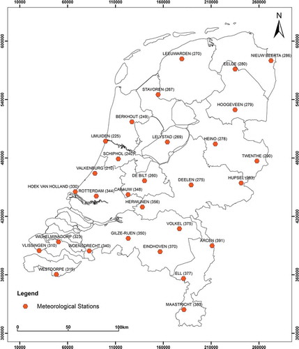
The wind dataset used in this study is obtained for free from the website of the Royal Netherlands Meteorological Institute (http://www.knmi.nl/klimatologie/uurgegevens/). This dataset contains hourly wind speed and direction for 34 weather stations in the Netherlands. For this study, we downloaded all available data from 2001 to 2010. A 10-year period is chosen as this is deemed sufficient to characterize wind resources (Soler-Bientz et al. 2009). Following international standards set by the World Meteorological Organization, the wind measurements are done at a height of 10 m and are representative of open terrain. Out of 34 stations, only 29 are finally selected for this study because more than 10% of data were missing in 5 stations. Figure 1 shows the distribution of the selected stations in the study area.

Figure 1. Distribution of the selected meteorological stations in the study area. The number between brackets after each station represents its unique ID.

2.2. Analytical workflow

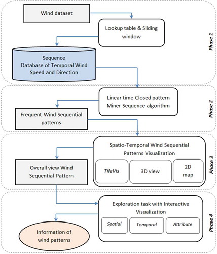
The analytical workflow used to mine and visualize sequential patterns in space and time consists of four phases: data preparation, frequent sequential pattern mining, spatio-temporal visualization and wind sequential patterns exploration (Figure 2). The next subsections describe in detail each of the four phases.

Figure 2. The four phases of the analytical workflow for interactively discover wind characteristics.

2.2.1. Phase 1: data preparation

Mining sequential patterns from wind speed and direction data requires the combination of these characteristics into a single variable by using a lookup table (Figure 3a). As explained in Yusof et al. (2014), the frequent sequential pattern algorithms cannot deal with multivariate datasets. The data also needs to be classified into a finite number of categories, depending on the application at hand (Pérez et al. 2004, Trusenkova et al. 2009). In this study, the wind speed and direction were respectively discretized into seven and eight classes according to the distribution ranges found in the wind dataset and each unique class combination was assigned a unique ID (Figure 3a). For instance, a combination of ID 1 (Speed class) with ID 1 (Direction class), and ID 1 (Speed class) with ID 2 (Direction class) were assigned to 01 and 02, respectively (Figure 3a). Thus, ID 01 represents wind speeds in the range of 0–4 m/s that come from the northeast (45°).

Figure 3. (a) The new IDs (itemsets) generated from the combination of wind speed and direction IDs, (b) the sliding window that moves along the list of itemsets according to the length_range (48) and step_v (24) parameter values, and (c) sequence database that consists of transactions (window 1, 2,…, n) and each transaction gets assigned a unique ID (TID).

These IDs (itemsets), along with their corresponding time stamp (hourly time unit), were then combined into temporally continuous sequences by using an SW. The SW is a temporal kernel that moves along the list of IDs (Figure 3b) to create sequences without having to split them according to arbitrary temporal units (e.g. days). These sequences were stored as rows in a sequence database (SD; Figure 3c). By doing this, each sequence can now be called a transaction and, therefore, it gets assigned a unique transaction ID (TID).

The SW processing depends of two parameters: length_range, step_v. Parameter length_range (n) is the unit distance between the pth itemset position and the qth itemset position (Figure 3b), assuming each itemset position is a time stamp (i.e. p = 1 h and q = 48 h, n = 48). A 48-h length allows extraction of patterns that can expand across more than a single day (across time continuation). To ensure that the sequences are not split by time, there are overlaps between two windows whenever the SW slides through the time series data. The size of the overlapping window is based on the second SW parameter, the step_v value (i.e. step_v = 24 h in Figure 3b). In this case, a 24-h step is chosen for retrieval of daily wind behaviour relationship, both before and after the overlapping period, and for exhaustive mining of all sequential patterns present in the data. Values of both length_range and step_v can be changed by users if required. Here we applied an SW (48, 24) for generating new ID sequences that were stored in the SD together with TIDs. Once the SD is ready, it is possible to apply the sequential pattern mining algorithm for extracting the wind sequential patterns.

2.2.2. Phase 2: frequent sequential pattern mining

The Linear time Closed pattern Miner Sequence (LCMSeq) algorithm (Uno et al. 2005) was used to mine the wind sequential patterns from the generated SD. The time LCMSeq takes to compute the patterns is linearly proportional to the size of the input database. The computation time for finding frequent itemsets only depends on the number of itemset found; if this number is large, then computation time for each itemset is relatively low. Besides, this frequent pattern algorithm only returns closed itemsets by eliminating patterns that are included in longer patterns and in the same frequency. This algorithm also provides fast frequent counting by implementing new data structure combining array list, bitmap and prefix tree (Uno et al. 2005). Hence, LCMSeq improves the computation time and the memory usage (Uno et al. 2005, Nakahara et al. 2010).

The generated SD (Section 2.2.1) is the input of the LCMSeq algorithm. To speed up the computation of the frequent patterns, the SD is transformed into a new structure in memory using three techniques: (a) a bitmap representation, which is a two-dimensional yes/no matrix setting transaction lists against itemset, denoting with ‘yes’ or ‘1’ all transactions whereby the corresponding itemset is a member; (b) a prefix tree, whereby the itemsets are stored in the nodes of a tree while whose leaves list the transactions where the pattern occurs and the search tree constructed by moving from the root of the tree till that leaf; and (c) an array of lists, whereby each element of the array stores the itemset of the pattern and the transactions where this pattern occurs. Each of these techniques is suited for a specific dataset (bitmap is suited for a dense dataset and a relatively large minimum support value, prefix tree is suited for a structured dataset and a large minimum support value, and array lists is suited for sparse datasets).

Additionally, we used three constraints, namely the minimum support threshold (ξ), length of time (L_t) and time gap (g) in the LCMSeq to extract wind patterns. These constraints are application specific, as they define the kind of patterns that will be mined. A sequence, S, is called a frequent sequential pattern if the total number of the transactions that contain S is equal to or greater than a user-specified minimum number. This number is the support threshold (ξ). If ξ is set too high, few patterns are discovered. For instance, for ξ equal to 48 only six patterns are found. Conversely, if ξ is set too low, it will generate a large number of patterns that would not only be difficult to analyse but also would not reflect truly frequent patterns. For instance, for ξ equal to 6 LCMSeq returns 166 patterns. Here, we empirically set ξ as equal to 24 because it provides a reasonable number of frequent patterns. The length time (L_t) is the minimum length of the sequential pattern. For this study, L_t was made equal to 24. This allows extraction of wind patterns that either fall in a single day or span two consecutive days. The time gap (g) constraint is used to prevent any gap between elements in the sequential patterns. Since we are interested in continuous patterns, we set the time gap to 0. Notice that the users can set different values for the constraint parameters (ξ and L_t). For instance, if users are interested with longer length of sequential patterns, the L_t value can be set as anything from greater than 24 to a maximum of 48 (based on SW length_range).

The outputs of the frequent pattern mining are the sequential patterns and their IDs. These IDs are composed of the TID in the SD and of the Time_start and Time_end (hour in this case) associated with the first and the last itemsets in the pattern. For instance, the ID <1, 20, 47> means that the pattern is found in the first transaction of the SD and the pattern takes place between the 20th and the 47th hours of the sequence. With this information, we can calculate the length of the pattern that, in this case, is equal to 28 h.

2.2.3 Phase 3: spatio-temporal visualization

The wind sequential patterns were depicted using visualizations that support the temporal and spatial aspects of wind data. To achieve this, we applied the concept of CMV (Roberts 2005). The individual views of a CMV environment contain different graphic representations of the same data to allow alternative perspectives. Interacting with one view will automatically affect other views.

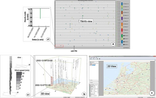
Three different visual representations were used in our CMV environment: TileVis, STC (including a 3D wind rose) and 2D geographical map (Figure 4). Moreover, the design of our environment followed the Focus + Context principle where Context delivers the full extent of spatio-temporal dataset (patterns), and Focus is a part of the dataset that has been temporally focused on details (Card et al. 1999, Carvalho et al. 2008). The next subsections describe in detail the three visual representations.

Figure 4. The interactive visualization tools used for wind pattern exploration: (a) overall view of the frequent wind sequential patterns in TileVis, (a1) a magnified view of the axes of TileVis, (b) a 3D view (STC) that allows visualizing wind speed and direction, (b1) A magnified view of one of the wind roses illustrated in the STC, and (c) a 2D map to show the stations that contain the patterns selected in TileVis.

TileVis

TileVis is designed to visualize temporal sequential patterns for a set of geographical locations. The locations (weather stations in this case) are represented by horizontal sub-Tiles which are arranged according to their ID number (Figure 4a). Positions and colours are used to encode information in each sub-Tile. The position along the horizontal axis refers to the temporal unit (day), and the vertical axis position represents temporal subunits of the temporal unit (here hours – Figure 4a1). For each sub-Tile, the vertical axis has a length of 48 h (see Section 2.2.1), and it is used to plot the hourly wind sequential patterns. This length is selected based on the length_range (48) set in the SW. The dotted line in each of the sub-Tile is used to separate the two days that it represents. The sub-Tiles are stacked on top of each other that correspond with a similar time interval in the horizontal axis. TileVis is an interactive visualization tool that allows selection of data by station and by the type of pattern. Using buttons, users can control the amount of information that they want to visualize in the TileVis. Figure 4a shows how the TileVis interface is used to visualize 4 of the 15 wind sequential patterns.

3D wind rose and space–time-cube

The 3D wind rose is based on the classic 2D wind rose concept and aims at providing a temporal view of the wind sequential patterns. The length and the facing direction of the rose bars represent the speed and direction, respectively. The vertical axis represents the time, with hourly values (Figure 4b1). The 3D wind rose has been implemented in a STC environment. It treats the time as the third dimension (vertical axis), while the two planar dimensions represent the geographical space (longitude, latitude) (Figure 4b). This STC facilitates the understanding of the reoccurring wind sequential patterns over times and indicates the stations where these patterns occurred. There are two ways of representing wind sequential patterns using the 3D wind rose: (i) a detailed representation for every wind sequential patterns in relation to their occurrences in space and time, and (ii) a generalization of wind sequential patterns generated from the detailed wind patterns. These two representations are further discussed in Sections 3.2.2 and 3.2.3.

2D map

This map is used as a base map in the 2D view and as reference map in the STC (Figure 4c and 4b). The map in the 2D view will display the locations of the stations that exhibit the same wind pattern. Additionally, the base map in the STC can be moved upwards and downwards along the vertical (time) axis. To have details on demand, the STC supports an operation called Spatio-Temporal zoom. The Spatio-Temporal zoom is used to enlarge the time axis according to the user-specified time (for instance, in range of time or specific time). This allows users to filter out non-relevant information and to explore parts of the sequential patterns.

Technical implementation

The TileVis was implemented using the Python programming language. The 2D map, the 3D wind rose in the STC were developed using open source ILWIS 3.08 software that can be downloaded at http://52north.org/communities/ilwis/ilwis-open/download. The visualizations were integrated in order to support direct linking between the multiple views. For instance, if a pattern is selected in TileVis, the STC will visualize the 3D wind rose that represents the selected pattern. This interactivity was realized using the so-called Dynamic Data Exchange, an interprocess communication functionality in Windows OS.

2.2.4. Phase 4: wind sequential patterns exploration

The mined patterns were further interpreted using three visual tasks (MacEachren 2004, Andrienko and Andrienko 2006), each focusing on a different dimension of the dataset:

• Spatial task: Identify stations that share similar (or dissimilar) wind characteristics. This task is achieved by first selecting the stations from the TileVis using the check button to visualize the wind sequential patterns in these locations on the STC. The 2D map shows the location of those selected stations.

• Temporal task: Identify patterns that occur in a specific time window. This task can be accomplished by selecting the start and end time in the TileVis. This provides information on both the type of patterns and their location in the STC and 2D map, respectively.

• Attribute task: Highlighting the predefined pattern of interest. The task is to select any pattern from the TileVis using the radio button. Then, the occurring times of the selected pattern can be identified in the STC, while their locations are highlighted in the 2D map.

3. Results and discussion

3.1. Wind sequential pattern mining results

After having removed all incomplete records from the original data, transforming the obtained data into a unique ID and applying the SW (Section 2.2.1), a total of 18,528 transactions were stored in the wind SD. The application of LCMseq, assuming ξ = 24, L_t = 24 and g = 0, led to the discovery of 488 occurrences of wind patterns belonging to 15 unique sequential patterns (Figure 6). These unique patterns consist of different durations that range from 24 to 48 h, and they describe wind speed and direction for different times of the day. It is remarkable that the number of patterns found using the SW approach is three times higher than the ones found by Yusof et al. (2014), who mined the same wind dataset after discretizing it into natural days (i.e. 24-h blocks) and used the same LCMSeq parameterization. This demonstrates the importance of not discretizing the time in sequential DM.

Figure 5. (a) TileVis visualization for overall wind sequential patterns distribution, (b) distribution of wind sequential patterns for stations 255, 240 and 249 in TileVis, (c) focusing wind patterns in selected time moment (from 25 to 30 December 2008), and (d) distribution of pattern 12 in all stations for the whole period of study.

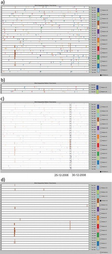
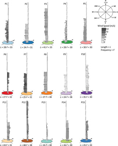
Figure 6. Visual representation of wind sequential patterns using 3D wind rose (P = pattern, L = length and F = frequency). Each of the 3D wind rose based is referred to pattern colours (refer to Figure 5).

3.2. Spatio-temporal wind sequential pattern visualization

3.2.1. Wind sequential patterns overview

The TileVis was used to get an overall view of the discovered patterns (Figure 5a). This visualization shows the distribution of the sequential patterns according to their weather stations and the time of their occurrences. Each wind sequential pattern is represented with a different colour code (pattern label). Users can use the check buttons and radio buttons to interactively select stations or patterns of interest. When the user selects a pattern, a typical follow-up question can be addressed; for instance, a question about which stations share similar patterns. This is where the TileVis will highlight those similar patterns as well as the corresponding stations that belong to these patterns. The details of pattern explorations using TileVis are presented in Section 3.3.

3.2.2. Wind sequential pattern in 3D wind rose

The wind patterns are further decomposed by showing their speed and direction using the 3D wind rose. Here, the speed is visualized using the visual variable values colour (grey scale). The lighter the grey colour, the lower the wind speed. Additionally, the length of the rose bar also shows the speed intensity and indicates the direction from which the wind blows. By using this 3D wind rose, we are able to illustrate the variability of the wind speed and direction at each time-stamp (in hours) from the extracted wind sequential patterns. The 3D wind roses for all the 15 unique patterns are shown in Figure 6. This figure illustrates the generalized wind sequential patterns calculated by averaging the wind speed and direction for all the stations where these patterns were found.

The results from Figure 6 show that the wind sequential patterns contain two prevailing wind directions blowing from the northeast-east(NE-E) (patterns 6, 10, 11, 12, 13, 14 and 15) and south-southwest(S-SW) (patterns 1, 2, 3, 4, 5, 7, 8 and 9). The obtained wind speed for the wind sequential patterns can be categorized into three levels – low, moderate and high. The lowest wind speed is 2–4 m/s (patterns 4, 9, 10 and 13). Moderate and high wind speed are 4–8 m/s and 9–12 m/s, respectively. Moderate wind speed is the most dominant speed recorded in 10 different wind sequential patterns (patterns 1, 2, 3, 5, 6, 8, 11, 12, 14 and 15). However, pattern 7 is the only pattern that has the highest wind speed in the study area.

In addition, patterns 8, 9 and 12 share the highest number of occurrences (38). However, these patterns have different durations where pattern 12 runs for of 48 h, and patterns 8 and 9 run for 27 and 24 h, respectively. For the entire period of study, pattern 8 distributions were found mostly at stations located far from the coastal area. The 3D wind rose shows that wind direction of this pattern blows from 190° to 210° (S-SW) with moderate wind speed, whereas stations that contain pattern 9 are mostly located in the eastern region of The Netherlands with the wind blowing from 190° to 220° (S-SW) direction. Pattern 9 has the lowest wind speed at 2–4 m/s. The weak wind speed in this pattern could be associated with the land use features such as built-up areas that can decrease the speed significantly. In pattern 12, the wind blows from 50° to 90° (NE-E) direction and is mostly distributed in the southwestern region of the study area. This pattern has a moderate wind speed of 5–8 m/s. Overall, we observed that both patterns 8 and 12 have potential availability of wind speed resources (10 m height) in the study area.

The 3D wind rose is useful not only for gaining the meaning of the sequential patterns, but also for incorporation into the geographical space to find out where and when such patterns occurred. The details are explained in Section 3.3.

3.2.3. 3D view of wind sequential patterns

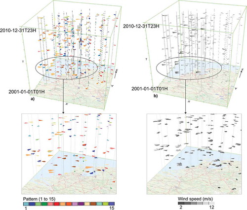
The wind sequential patterns were further explored using the STC. This view incorporates space, time and wind categorical components (speed, direction and wind pattern). This way, the wind sequential patterns can be explored in their geographic location and distribution in chronological order of time. To provide detailed information of the wind patterns, the wind categorical components comprising of speed, types of pattern and direction are represented by the length of the rose bars, colours and the facing direction of the rose bars, respectively (Figure 7). Notice that in this figure the 3D rose bars appear as thin disks because these roses represent events that occurred over a relatively short time interval (e.g. 48 h over 10 years). This representation is used to prevent visual cluttering while still providing an overview of all the mined patterns.

Figure 7. Wind sequential patterns illustrated using 3D wind roses and coloured according to (a) the type of pattern, and (b) to their speed (m/s).

Additionally, the STC and 2D map are linked to the TileVis to provide the interactivity for wind sequential patterns exploration. This means that the user can select part of the data (i.e. station or pattern) in TileVis and the selected data will be shown simultaneously in the STC or in the 2D map for further investigation.

Visualizing a large number of wind sequential patterns can result in overplotting, which makes it difficult for the users to track the numerous visual elements. To mitigate this and to allow the exploration of the patterns, the visual environment is designed based on the Focus + Context principles. The TileVis can serve as the context of the overall sequential patterns corresponding to the collection of sub-Tiles. Hence, the TileVis is used to visualize the entire set of wind sequential patterns at once. This helps the users to see relevant patterns on the display in such a way that significant patterns are detectable and preserved. Meanwhile, the STC serves as the focus of the TileVis, where detailed information (wind speed, direction, type of patterns and time of occurrences) on the TileVis selection are displayed. The 2D map is also treated as a focus element as it only highlights the selected stations of interest.

3.3 Wind sequential pattern exploration

3.3.1. Spatial visual task: revealing patterns that belong to area of interest

Corresponding patterns to the specific area might appear while monitoring spatio-temporal changes in wind characteristics. The users can refer to a single location or part of the area by specifying the station name or spatial relation such as stations in area X. For this task, the formulated questions can be, ‘What is the trend of wind patterns at station 225?’ or, ‘How do the wind patterns look like for stations that are located in the province of North Holland?’ The results are treated in the sense of discovering similarities and differences in wind sequential patterns within the selected locations.

To achieve this, the users can use the TileVis view to select the station of interest, using the check buttons. Figure 5b illustrates three selected stations in the TileVis, namely, stations 225, 240 and 249 located in the North Holland province. In the STC, only the wind sequential patterns belonging to these stations were visualized, while the others remained invisible (Figure 8b). This allows the users to focus on trends for those stations. Figure 8a shows the position of the selected stations highlighted as square symbol.

Figure 8. Wind sequential patterns in 3D view and 2D map: (a) the 2D map shows the positions of the selected stations highlighted in square symbol, and (b) occurring wind sequential patterns over time which visualized on top of the stations.

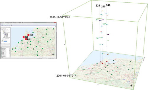
From Figures 5b and 8, we observe that each of the station shows various wind sequential patterns. Even though the stations are located in the same province, the wind characteristics show that they are different from each other. These differences lead to the assumption that these trends could be related to the geographical conditions (Figure 8a). For instance, station 240 (Schiphol), which is located in Schiphol International Airport tower, shows various wind patterns, while station 225 (IJmuiden) that is located in a coastal area has less numbers of frequent patterns compared to station 240. These trends show the influence of geographical conditions that cause different wind pattern occurrences, leading to heterogeneous wind behaviour in the spatial context.

3.3.2. Temporal visual task: identifying patterns in selected time interval

One of the important questions users might have is what types of wind sequential patterns are present during a certain time interval. For such a task, our proposed tools allow one to perform a time interval selection for identifying stations and the patterns that occur in the selected period. Consider the following question addressing one particular time interval; what patterns occurred during the whole day between 25 and 30 December 2008 at all stations? The time interval was selected in TileVis (Figure 5c), and the occurring patterns during this selected period is then identified from the STC and 2D map (Figure 9).

Figure 9. Wind sequential pattern occurrences during the selected time interval: (a) highlighted stations indicate stations that contain at least one of the selected patterns, (b) wind sequential patterns occurrences in time with different patterns in STC, and (c) visualizing wind speed and direction for reoccurring pattern 11 (red dot line).

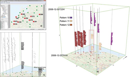
Figure 9a shows that there are three sequential patterns, namely, patterns 10, 11 and 12 occurring in 10 different stations. Most of them appeared only once except for station 240 where pattern 11 (in red dotted line) occurred twice. This explains that within this time interval, we could observe similar wind behaviour occurring not only in different stations, but also in similar stations (red dotted line) (Figure 9b). Additionally, the wind direction of these patterns shares similar behaviour where the wind is coming mostly from the northeast direction. This indicates that wind direction is more consistent than wind speed during the selected time interval. To observe the vagaries of wind speed visually, the representation of the 3D wind rose can be changed using the speed attribute. For instance, Figure 9c depicts the changes of wind speed for pattern 11 (red dotted line) ranging from 2 to 8 m/s, with the wind blowing in the direction of 60° to 80° (NE).

3.3.3. Attribute visual task: highlighting the predefined pattern of interest

Contrary to the first and second tasks, revealing similar wind patterns also provide useful information on the wind behaviour. Since the chosen patterns are known, one can determine their times of recurrence and identify the station that exhibits a particular pattern. The existence of similar patterns at individual station or set of stations might point to the possibility of common conditions at their locations. Additionally, the users can observe any repetitive wind pattern distributed over times to detect regular wind behaviour which can be expected every day or month. For such task, the users may select any pattern of interest by using the radio button on the right side of the TileVis. For this task, we have chosen the longest sequential pattern, which is pattern 12, to discover the wind behaviour. Figures 5d and 10a demonstrate the overall distribution of pattern 12 in TileVis and STC in all weather stations, respectively. In Figure 5d, the pattern occurs for four consecutive days (from 7 to 11 December 2002) in station 344. For stations 340 and 348, the pattern appeared for three days in a row (from 7 to 10 December 2002). This shows that stations 340, 344 and 348 share similar wind characteristics for the same time period. We observed that the surrounding areas of these weather stations share common geographic characteristics. The stations are located in open areas characterized by grassland and arable land with few obstacles to deflect the wind flow. The repetitive occurrences of pattern 12 appeared mostly in December 2002, indicating that regular wind behaviour persisted continuously for a couple of days.

Figure 10. Similar wind pattern occurrences: (a) 2D map highlights the stations that contain pattern 12 with square symbol (red colour), (b) distribution of pattern 12 for the whole period of study, and (c) reoccurring pattern 12 in the selected time period (blue dot box in 10b).

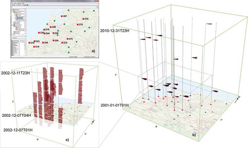
To depict details of wind behaviour for pattern 12 in December 2002 (from 7 to 11 December 2002), the STC time window was set to this time period (area inside the blue box in Figure 10b). To focus only on these selected time intervals, spatio-temporal zoom tool in STC is used to zoom in through the selected time with respect to location (stations) and the wind pattern components (Figure 10c). The occurring times for the displayed patterns can be identified by moving the reference map towards the above direction and stopping at where it took place. The time of the occurrence pattern is displayed at the vertical axis of the cube (Figure 10c). Figure 10c illustrates the pattern’s direction is from 50° to 90° (NE-E) during this time period.

4. Conclusion

In this paper, a novel approach to mine and interactively discover sequential patterns in wind data has been developed. This approach has three main hallmarks. First, it facilitates the process of mining temporal wind data through analysis of wind speed and direction simultaneously. Hence, the mining process will be more efficient and faster in a single process. Second, it allows for an efficient detection of all the sequential patterns present in the data by combining a state-of-the-art mining algorithm (LCMSeq) with a time SW. The use of such an SW avoids the discretization of data into arbitrary time units (e.g. daily wind values), thereby preventing the loss of patterns that occur across multiple time units. The implemented mining process is generic, and users can empirically fine-tune the LCMSeq and SW parameters to mine different sequential wind patterns according to their needs or the target application. Third, the proposed discovery of wind sequential patterns demonstrates the capabilities of data visualization to convey an overview. Moreover, the interactive character of the visualizations leads to new insights that could not be obtained from the original data or from the wind patterns alone. The three visual tasks help the user to explore the wind patterns at multiple levels of details (Focus + Context), and the use of multiple views (TileVis, 3D and 2D) minimizes the time needed to understand wind behaviour as each view provides a different perspective of the wind behaviour.

The approach was applied to 10 years of hourly wind measurements in the Netherlands where we found 15 wind sequential patterns. These patterns were further explored using interactive visualizations and by way of three tasks. The spatial task showed that weather stations located in the same province do not necessarily experience similar wind patterns. Meanwhile, the temporal task revealed that within the selected time interval, we are able to find similar wind behaviour occurring not only in different stations but also in the same station at different times of occurrences. The attribute task revealed the repetition of the chosen wind pattern, indicating as regular wind behaviour at different weather stations that persists continuously for some period. Overall, the conducted wind pattern explorations are about harnessing the user’s visual perception capabilities so that these can identify trends, patterns or any unusual occurrences in wind behaviour. The exploration results provide qualitative information of wind behaviour in relation to the spatial, temporal and attribute dimensions. Besides, the generated wind patterns yields users with generic ideas of areas or periods that might require further investigation, and/or analysis, which in turn can provide useful insights and knowledge to experts or decision-makers. In this regard, future researches might be geared towards testing by wind domain experts for validation of the overall proposed works.

Acknowledgments

The authors would also like to acknowledge The Royal Netherlands Meteorological Institute (KNMI) for providing the wind data.

Disclosure statement

No potential conflict of interest was reported by the authors.

Additional information

Funding

This work was supported by the Malaysian Ministry of Education (SLAI) and Universiti Teknologi Malaysia (UTM).

References

- Aigner, W., et al. 2011. Visualization of time-oriented data. London: Springer-Verlag London Limited: Springer.
- Andrienko, N. and Andrienko, G., eds. 2006. Exploratory analysis of spatial and temporal data - a systematic approach. Berlin: Springer-Verlag.
- Archer, C.L. and Jacobson, M.Z., 2013. Geographical and seasonal variability of the global “practical” wind resources. Applied Geography, 45 (0), 119–130. doi:10.1016/j.apgeog.2013.07.006
- Bach, B., et al., 2014. A review of temporal data visualizations based on space-time cube operations. Eurographics conference on visualization, 9 June 2014 Swansea, Wales, United Kingdom.
- Boukhelifa, N. and Rodgers, P.J., 2003. A model and software system for coordinated and multiple views in exploratory visualization. Information Visualization, 2 (4), 258–269. doi:10.1057/palgrave.ivs.9500057
- Card, S.K., Mackinlay, J.D., and Shneiderman, B., eds. 1999. Readings in information visualization: using vision to think. San Francisco, CA: Morgan Kaufmann Publishers.
- Carvalho, A., et al., 2008. A temporal focus + Context visualization model for handling valid-time spatial information. Information Visualization, 7 (3–4), 265–274. doi:10.1057/palgrave.ivs.9500188
- Chen, Y.-L., Chiang, M.-C., and Ko, M.-T., 2003. Discovering time-interval sequential patterns in sequence databases. Expert Systems with Applications, 25 (3), 343–354. doi:10.1016/S0957-4174(03)00075-7
- Chen, Y.-L. and Hu, Y.-H., 2006. Constraint-based sequential pattern mining: the consideration of recency and compactness. Decision Support Systems, 42 (2), 1203–1215. doi:10.1016/j.dss.2005.10.006
- Colak, I., Sagiroglu, S., and Yesilbudak, M., 2012. Data mining and wind power prediction: A literature review. Renewable Energy, 46, 241–247. doi:10.1016/j.renene.2012.02.015
- Das, G., et al., 1998. Rule discovery from time series. In: Proceedings of the Fourth ACM SIGKDD international conference on knowledge discovery and data mining, 27–31 August New York. New York: American Association for Artificial Intelligence, 16–22.
- de Oliveira, M.C.F. and Levkowitz, H., 2003. From visual data exploration to visual data mining: a survey. IEEE Transactions on Visualization and Computer Graphics, 9 (3), 378–394. doi:10.1109/TVCG.2003.1207445
- Demšar, U., et al., 2015. Stacked space-time densities: a geovisualisation approach to explore dynamics of space use over time. GeoInformatica, 19 (1), 85–115. doi:10.1007/s10707-014-0207-5
- Gotz, D., Wang, F., and Perer, A., 2014. A methodology for interactive mining and visual analysis of clinical event patterns using electronic health record data. Journal of Biomedical Informatics, 48, 148–159. doi:10.1016/j.jbi.2014.01.007
- Helbig, C., et al., 2014. Concept and workflow for 3D visualization of atmospheric data in a virtual reality environment for analytical approaches. Environmental Earth Sciences, 72 (10), 3767–3780. doi:10.1007/s12665-014-3136-6
- Hernández-Escobedo, Q., et al., 2014. Wind energy resource in Northern Mexico. Renewable and Sustainable Energy Reviews, 32, 890–914. doi:10.1016/j.rser.2014.01.043
- Hu, T., et al., 2008. Discovery of maximum length frequent itemsets. Information Sciences, 178 (1), 69–87. doi:10.1016/j.ins.2007.08.006
- Hu, Y.-H., et al., 2009. On mining multi-time-interval sequential patterns. Data & Knowledge Engineering, 68 (10), 1112–1127. doi:10.1016/j.datak.2009.05.003
- Huisman, O., et al., 2009. Developing a geovisual analytics environment for investigating archaeological events: extending the space-time cube. Cartography and Geographic Information Science, 36 (3), 225–236. doi:10.1559/152304009788988297
- Javaheri, S.H., Sepehri, M.M., and Teimourpour, B., 2014. Chapter 6 - response modeling in direct marketing: A data mining-based approach for target selection. In: Y. Zhao and Y. Cen, eds. Data mining applications with R. Boston, MA: Academic Press, 153–180.
- Ji, X., Bailey, J., and Dong, G., 2007. Mining minimal distinguishing subsequence patterns with gap constraints. Knowledge and Information Systems, 11 (3), 259–286. doi:10.1007/s10115-006-0038-2
- Jung, J. and Tam, K.-S., 2013. A frequency domain approach to characterize and analyze wind speed patterns. Applied Energy, 103, 435–443. doi:10.1016/j.apenergy.2012.10.006
- Kainkwa, R.M.R., 2000. Wind speed pattern and the available wind power at Basotu, Tanzania. Renewable Energy, 21 (2), 289–295. doi:10.1016/S0960-1481(00)00076-8
- Keefe, D., et al., 2009. Interactive coordinated multiple-view visualization of biomechanical motion data. IEEE Transactions on Visualization and Computer Graphics, 15 (6), 1383–1390. doi:10.1109/TVCG.2009.152
- Kehrer, J. and Hauser, H., 2013. Visualization and visual analysis of multifaceted scientific data: a survey. IEEE Transactions on Visualization and Computer Graphics, 19 (3), 495–513. doi:10.1109/TVCG.2012.110
- Keogh, E., et al., 2006. Finding the most unusual time series subsequence: algorithms and applications. Knowl Information Systems, 11 (1), 1–27. doi:10.1007/s10115-006-0034-6
- Kraak, M.J., 2008. Geovisualization and time: new opportunities for the space - time cube. In: M. Dodge, M. McDerby, and M. Turner, eds. Geographic visualization: concepts, tools and applications. Chichester: John Wiley & Sons, 293–306.
- Kum, H.-C., et al., 2003. ApproxMAP: approximate mining of consensus sequential patterns. In: Proceedings of the 2003 SIAM International Conference on Data Mining (SDM ’03). 1–3 May 2003 Cathedral Hill Hotel, San Francisco, CA: SIAM 311–315.
- Kum, H.-C., Chang, J., and Wang, W., 2006. Sequential pattern mining in multi-databases via multiple alignment. Data Mining and Knowledge Discovery, 12 (2–3), 151–180. doi:10.1007/s10618-005-0017-3
- Kusiak, A., Haiyang, Z., and Zhe, S., 2009. Short-term prediction of wind farm power: A data mining approach. IEEE Transactions on Energy Conversion, 24 (1), 125–136. doi:10.1109/TEC.2008.2006552
- Landberg, L., 1999. Short-term prediction of the power production from wind farms. Journal of Wind Engineering and Industrial Aerodynamics, 80 (1–2), 207–220. doi:10.1016/S0167-6105(98)00192-5
- Liu, H., Erdem, E., and Shi, J., 2011. Comprehensive evaluation of ARMA–GARCH(-M) approaches for modeling the mean and volatility of wind speed. Applied Energy, 88 (3), 724–732. doi:10.1016/j.apenergy.2010.09.028
- Liu, Y. and Weisberg, R.H., 2005. Patterns of ocean current variability on the West Florida Shelf using the self-organizing map. Journal of Geophysical Research: Oceans, 110 (C6), C06003. doi:10.1029/2004JC002786
- MacEachren, A.M., ed. 2004. How maps work: representation, visualization, and design. New York: Guilford Press.
- Mann, D., Lant, C., and Schoof, J., 2012. Using map algebra to explain and project spatial patterns of wind energy development in Iowa. Applied Geography, 34 (0), 219–229. doi:10.1016/j.apgeog.2011.11.008
- Miranda, M.S. and Dunn, R.W., 2006. One-hour-ahead wind speed prediction using a Bayesian methodology. In: 2006 Power engineering society general meeting, 18–22 June Montreal, QC. New York: Institute of Electrical and Electronics Engineers (IEEE), 3557–3562.
- Nakahara, T., Uno, T., and Yada, K., 2010. Extracting promising sequential patterns from RFID data using the LCM sequence. In: R. Setchi, et al. eds. Knowledge-based and intelligent information and engineering systems. Berlin Heidelberg: Springer, 244–253.
- Nöllenburg, M., 2007. Geographic visualization. In: A. Kerren, A. Ebert, and J. Meyer, eds. Human-centered visualization environments. Berlin, Heidelberg: Springer, 257–294.
- Orellana, D., et al., 2012. Exploring visitor movement patterns in natural recreational areas. Tourism Management, 33 (3), 672–682. doi:10.1016/j.tourman.2011.07.010
- Pérez, I.A., et al., 2004. Analysis of height variations of sodar-derived wind speeds in Northern Spain. Journal of Wind Engineering and Industrial Aerodynamics, 92 (10), 875–894. doi:10.1016/j.jweia.2004.05.002
- Pughazendi, N. and Punithavalli, D.M., 2011. Temporal databases and frequent pattern mining. International Journal of P2P Network Trends and Technology (IJPTT), 1 (1), 13–17.
- Risien, C.M., et al. 2004. Variability in satellite winds over the Benguela upwelling system during 1999–2000. Journal of Geophysical Research: Oceans, 109, 1–15. doi:10.1029/2003JC001880
- Roberts, J.C., 2005. Chapter 8 - exploratory visualization with multiple linked views. In: J. Dykes, A.M. MacEachren, and M.-J. Kraak, eds. Exploring geovisualization. Oxford: Elsevier, 159–180.
- Roberts, J.C., 2007. State of the art: coordinated & multiple views in exploratory visualization. Fifth International Conference on Coordinated and Multiple Views in Exploratory Visualization, CMV 2007, 2 July 2007 Zurich, Switzerland, 61–71.
- Robinson, A.C., 2011. Highlighting in geovisualization. Cartography and Geographic Information Science, 38 (4), 373–383. doi:10.1559/15230406384373
- Soler-Bientz, R., Watson, S., and Infield, D., 2009. Preliminary study of long-term wind characteristics of the Mexican Yucatán Peninsula. Energy Conversion and Management, 50 (7), 1773–1780. doi:10.1016/j.enconman.2009.03.018
- Tanbeer, S.K., et al., 2009. Sliding window-based frequent pattern mining over data streams. Information Sciences, 179 (22), 3843–3865. doi:10.1016/j.ins.2009.07.012
- Tandeo, P., et al., 2014. Combining analog method and ensemble data assimilation: application to the Lorenz-63 chaotic system. 4th International Workshop on Climate Informatics. 25–26 September 2014 Boulder, Colorado, USA: Springer, 3–12.
- Theisel, H., 2000. Higher order parallel coordinates. In: Proceedings of the conference on vision modeling and visualization, 22–24 November 2000, Saarbrücken, Germany: 415–420.
- Tominski, C., Abello, J., and Schumann, H., 2004. Interactive poster: 3D axes-based visualizations for time series data. In: Poster compendium of IEEE symposium on information visualization (InfoVis), 10–12 October Austin, TX. Orlando, FL: IEEE Computer Society, 49–50.
- Trusenkova, O., Nikitin, A., and Lobanov, V., 2009. Circulation features in the Japan/East Sea related to statistically obtained wind patterns in the warm season. Journal of Marine Systems, 78 (2), 214–225. doi:10.1016/j.jmarsys.2009.02.019
- Turdukulov, U., et al., 2014. Visual mining of moving flock patterns in large spatio-temporal data sets using a frequent pattern approach. International Journal of Geographical Information Science, 28 (10), 2013–2029. doi:10.1080/13658816.2014.889834
- Uno, T., Kiyomi, M., and Arimura, H., 2005. LCM ver.3: collaboration of array, bitmap and prefix tree for frequent itemset mining. In: Proceedings of the 1st international workshop on open source data mining: frequent pattern mining implementations, 21–24 August 2005 Chicago, Illinois: ACM. 77–86.
- Velo, R., López, P., and Maseda, F., 2014. Wind speed estimation using multilayer perceptron. Energy Conversion and Management, 81, 1–9. doi:10.1016/j.enconman.2014.02.017
- Verma, K. and Vyas, O.P., 2005. Efficient calendar based temporal association rule. SIGMOD Record, 34 (3), 63–70. doi:10.1145/1084805
- Wang, Z. and Yuan, X., 2014. Urban trajectory timeline visualization. In: 2014 International Conference on Big Data and Smart Computing (BIGCOMP), 15–17 January 2014 Bangkok, Thailand: Chatrium Hotel Riverside, 13–18.
- Yusof, N., et al., 2014. Mining frequent spatio-temporal patterns in wind speed and direction. In: J. Huerta, S. Schade, and C. Granell, eds. Connecting a digital Europe through location and place. Cham: Springer International Publishing, 143–161.
- Zaki, M.J., Carothers, C.D., and Szymanski, B.K., 2010. VOGUE: A variable order hidden Markov model with duration based on frequent sequence mining. ACM Transactions Knowl Discovery Data, 4 (1), 1–31. doi:10.1145/1644873
- Zhang, J., Gruenwald, L., and Gertz, M., 2009. VDM-RS: A visual data mining system for exploring and classifying remotely sensed images. Computers & Geosciences, 35 (9), 1827–1836. doi:10.1016/j.cageo.2009.02.006
- Zhang, Q., et al., 2013. Visual analysis design to support research into movement and use of space in Tallinn: A case study. Information Visualization, 13 (3), 213–231.