Climatic niche breadth can explain variation in geographical range size of alpine and subalpine plants

ABSTRACT

Understanding the environmental factors determining the distribution of species with different range sizes can provide valuable insights for evolutionary ecology and conservation biology in the face of expected climate change. However, little is known about what determines the variation in geographical and elevational ranges of alpine and subalpine plant species. Here, we examined the relationship between geographical and elevational range sizes for 80 endemic rhododendron species in China using Spearman’s rank-order correlation. We ran the species distribution model – maximum entropy modelling (MaxEnt) – with 27 environmental variables. The importance of each variable to the model prediction was compared for species groups with different geographical and elevational range sizes. Our results showed that the correlation between geographical and elevational range sizes of rhododendron species was not significant. Climate-related variables were found to be the most important factors in shaping the distributional ranges of alpine and subalpine plant species across China. Species with geographically and elevationally narrow ranges had distinct niche requirements. For geographical ranges, the narrow-ranged species showed less tolerance to niche conditions than the wide-ranged species. For elevational ranges, compared with the wide-ranged species, the narrow-ranged species showed an equivalent niche breadth, but occurred at different niche position along the environmental gradient. Our findings suggest that over large spatial extents the elevational range size can be a complementary trait of alpine and subalpine plant species to geographical range size. Climatic niche breadth, especially the range of seasonal variability, can explain species’ geographical range sizes. Changes in climate may influence the distribution of rhododendrons, with the effects likely being felt most by species with either a narrow geographical or narrow elevational range.

KEYWORDS:

• Biogeography
• niche breadth
• geographical range size
• elevational range size
• rhododendron
• China

1. Introduction

Global climate change is expected to have an impact on the distribution of species (Thomas et al. 2004, Parmesan 2006). Given the overall recorded rise in temperature, there are two likely consequences for species that are limited in their distribution by temperature constraints. Some species may shift their ranges to higher altitudes or higher latitudes, whereas others may experience a decrease or even extinction due to their slow migration rates or the limited availability of new habitat that results from the synergistic effects of a narrow niche and small range size (Ohlemuller et al. 2008, Chen et al. 2011, Lenoir and Svenning 2015). Although individual species may have idiosyncratic responses to climate change, species that share the same ecological trait might respond in the same way (Thuiller et al. 2005). Range size – reflecting interspecific differences of ecological tolerance, dispersal ability and evolutionary history – is a basic unit in biogeography and can be considered to be a species trait (Thompson et al. 1999, Olalla-Tarraga et al. 2011). The size of a species range is, at least partially, a spatial representation of its degree of specialization (Devictor et al. 2010). Range size has been used to predict the global extinction risk (Purvis et al. 2000, Botts et al. 2013) and the factors determining species’ range sizes likely affect their capacity to alter their ranges in response to climate change (Thomas et al. 2001, McCauley et al. 2014). Consequently, understanding the environmental factors determining the distribution of species with different range sizes can provide valuable insights for evolutionary ecology and conservation biology in the face of expected climate change.

Why some species have highly restricted geographic ranges while closely related species have widespread distributions has long fascinated ecologists and biologists (Brown et al. 1996, Gaston 1996). A variety of hypotheses and paradigms have been proposed to explain the variation seen in geographical range sizes between species, including climatic variability (Stevens 1989), evolution (Gaston 1996), complex interactions (Brown et al. 1996), niche breadth (Gaston et al. 1997, Gaston and Spicer 2001), energy availability (Morin and Chuine 2006), climate tolerance (Pither 2003), glacial history (Jansson 2003), colonization ability (Lowry and Lester 2006), and a combination of habitat area and climate stability (Morueta-Holme et al. 2013). Among these hypotheses, the niche breadth hypothesis, which has recently gained more support, suggests a positive correlation between niche breadth and geographical range size (Boulangeat et al. 2012, Botts et al. 2013). Brown (1984) indicated that species which can utilize a greater array of resources and that can maintain viable populations under a wider variety of conditions should become more widespread. Based on this, the niche breadth hypothesis states that species with a broad niche can persist in a wide range of different habitat types, while species with a narrow niche will be restricted to those places where their specific niche requirements are met.

Botts et al. (2013) and Slatyer et al. (2013) defined three general categories for the niche breadth: climate tolerance, habitat tolerance and diet. In terms of climate tolerance, Stevens (1989) proposed that species able to tolerate a larger climate variation should occupy larger geographical areas than species with less tolerance. In addition, the climate extreme hypothesis (represented by the lowest temperature of the coldest month or quarter) also gained support in some studies (Pither 2003, Kreyling et al. 2015). Meanwhile, climate- and soil-related variables are often used together as representations of habitat in species’ range size studies (Kockemann et al. 2009, Pannek et al. 2013). The reasoning is that climatic and edaphic variables are the functional variables of temperature and water and nutrient availability that limit the growth and distribution of plants (Munns 2002). Thus, tolerance to a wide range of climatic and edaphic conditions should be associated with greater range sizes (Morin and Lechowicz 2013). Furthermore, topography also contains information about a region’s climatic history, hydrology and geodynamics, and it determines the light available for plant growth. It is, therefore, often considered as a representation of habitat. In addition, topographical barriers are physiological barriers for species dispersal and affect distribution patterns, including range sizes (Janzen 1967, Ghalambor et al. 2006).

However, the relative importance of these basic factors of ‘niche breadth’ (i.e. climate, topography and soil) in shaping the distribution of plant species with different range sizes is unclear. The question is whether these basic factors are equally important in explaining the distribution of narrow- and wide-ranged species within a large extent? Or is climate alone more important for the narrow-ranged species that are expected to be more sensitive to climate change? Additionally, the term ‘climate’ refers to a diverse set of measurable variables. It matters which variables are important for the distribution of a species if we want to determine the impact of projected trajectories of climatic change on species’ shifts in ranges.

In recent years, alpine and subalpine plant species have increasingly become a conservation concern because it is anticipated they will be affected by climate change (Theurillat and Guisan 2001, Pérez-García et al. 2013). Alpine and subalpine plant species that cover a wide geographical range could also be expected to cover a wide elevational range (Blackburn and Ruggiero 2001). However, a species with a narrow geographical range might still occupy a wide elevational range, for example, when it occupies one specific but long hill or mountain slope. This may lead to different conclusions about which environmental factors are most important for species with a given range size. Interestingly, most macroecological studies have only considered geographical ranges, while the relationship between geographical and elevational range sizes has been less well studied (McCain 2006). Very few studies have related these two types of range sizes together. Blackburn and Ruggiero (2001) showed that there was a strong correlation between geographical and elevational range size for Andean passerines, while McCain (2006) reported no relationship between geographical and elevational ranges for Costa Rican rodents. White and Bennett (2015) recently found that elevational range size is a strong independent predictor of extinction risk that is complementary to geographical range size.

In this study, we examined the factors that control the subcontinental distribution of a key alpine and subalpine genus, the Rhododendron (Ma et al. 2014). The rhododendron genus forms a major component of vegetation in the Himalayan alpine zone (Li et al. 2013, Ma et al. 2014). Moreover, rhododendrons display a great variation in range size (Kumar 2012). Some rhododendron species occur throughout most of the northern hemisphere, while others are highly restricted to small regions. A number of rhododendron species have a wide elevational range, from 800 to 3000 m, while other species only grow in the upper part of the montane zone (Liang and Eckstein 2009). The rhododendron species’ large variation in geographical and elevational range sizes, and their dominant role in alpine and subalpine ecosystems, makes the rhododendron an ideal genus to test how climatic, topographic and edaphic variables shape the distribution of narrow- and wide-ranged species.

This study addresses three inter-related questions: (1) Do alpine and subalpine plant species with narrow geographical ranges also have narrow elevational ranges? (2) Are climatic, topographic and edaphic variables equally important in determining the distribution of alpine and subalpine plant species with different range sizes? (3) What factors determine the variation in geographical and elevational ranges of alpine and subalpine plant species?

2. Methods

2.1. Study area and species data

The study area covers the whole of China (Figure 1). China harbours about 542 rhododendron species, which are widely distributed across most regions (except Xinjiang and Ningxia provinces) with a wide range of climatic, topographic and edaphic conditions. Records on rhododendron presence were collected from seven herbaria and botanical museums (Herbarium of the Institute of Botany, Herbarium of the Kunming Institute of Botany, South China Botanical Garden, Wuhan Botanical Garden, Sichuan University of Botany, Sichuan Forest School and Lushan Botanical Garden). Because a high locational accuracy is required for studying plant species distribution, all records with inadequate descriptions of the location (e.g. mentioning only a county or mountain) were excluded. Our resulting dataset with 406 species comprised 13,126 georeferenced records with a spatial uncertainty of less than 1 km.

Figure 1. Study area and the locations of 80 rhododendron species in China used in the species distribution models.

2.2. Environmental variables

We collected climatic, topographic and edaphic data from a number of sources, and included a total of 27 variables (Table 1). For the climatic data, we used the bioclim variables (Hijmans et al. 2005, available at http://www.worldclim.org) which are based on the current (1950–2000) conditions at 30 arc-seconds resolution (~1 km at the equator). The digital elevation model (DEM) was derived from the SRTM (http://www.cgiar-csi.org/data/srtm-90m-digital-elevation-database-v4-1#download), with a resolution of 90 m. Slope gradient and aspect were calculated from the DEM using Horn’s algorithm in ArcGIS10.2 (ESRI, Inc., Redlands, California, USA). Edaphic data was collected from the global 3D soil information system SoilGrid at 1 km spatial resolution (ftp://ftp.soilgrids.org/; Hengl et al. 2014). From the available data layers, we selected soil pH, organic carbon and soil texture (i.e. sand, silt and clay fraction). The mean value of organic carbon was based on a depth of 0–30 cm, because the content of organic carbon decreases with the soil depth, and the top 20 cm is the layer which has the highest correlation of soil organic carbon and vegetation type (Jobbagy and Jackson 2000). Given that rhododendrons cover many life forms, we selected the 30–60 cm depth for measuring the other soil characters (i.e. soil pH and soil texture, Hengl et al. 2014). We used 1 km as a standard resolution for all the environmental variables because this is the highest resolution SoilGrid provides.

Table 1. Environmental variables used for modelling the distribution of rhododendrons.

Category	Variable	Abbreviation	Unit
Climate	Annual mean temperature	Bio1	°C
	Mean diurnal range	Bio2	°C
	Isothermality	Bio3	-
	Temperature seasonality	Bio4	°C
	Max temperature of warmest month	Bio5	°C
	Min temperature of coldest month	Bio6	°C
	Temperature annual range	Bio7	°C
	Mean temperature of wettest quarter	Bio8	°C
	Mean temperature of driest quarter	Bio9	°C
	Mean temperature of warmest quarter	Bio10	°C
	Mean temperature of coldest quarter	Bio11	°C
	Annual precipitation	Bio12	mm
	Precipitation of wettest month	Bio13	mm
	Precipitation of driest month	Bio14	mm
	Precipitation seasonality	Bio15	–
	Precipitation of wettest quarter	Bio16	mm
	Precipitation of driest quarter	Bio17	mm
	Precipitation of warmest quarter	Bio18	mm
	Precipitation of coldest quarter	Bio19	mm
Topography	Elevation	Elev	m
	Northness	North	–
	Slope	Slope	degree
Soil	Soil organic carbon (dry combustion)	OrcC	g kg^−1
	pH index(H2O solution)	pH	10^−^1
	Sand content (gravimetric)	Sand	kg kg^−1
	Silt content (gravimetric)	Silt	kg kg^−1
	Clay content (gravimetric)	Clay	kg kg^−1

2.3. Species distribution modelling

Species distribution models (SDMs) have often been used to assess the importance of environmental variables in explaining species distributions. In this study, we used maximum entropy modelling (MaxEnt, version 3.3.3e, Phillips et al. 2006) because it generally performs well with presence-only species records (Phillips and Dudik 2008), and it provides appropriate background samples to deal with sample biases (Prates-Clark et al. 2008, Elith et al. 2011). Because our data were collected from seven herbaria and botanical museums which hold rhododendron records over more than 50 years, we would consider absences in certain regions reflect absences of rhododendron, rather than absence of sampling effort.

When fitting SDMs, there is ideally no strong correlation between the explanatory variables, that is, no collinearity. If our aim is to predict the distribution of rhododendrons, we cannot do any analysis without eliminating the multicollinearity. However, we focus on the determining factors of rhododendrons with different range sizes, a priori information about selecting the determining factor was not available for rhododendrons. Therefore, excluding variables from our analysis would be mainly subjective. In addition, MaxEnt has an internal procedure to handle multicollinearity of environmental variables, which has been verified by a number of studies (Prates-Clark et al. 2008, Elith et al. 2011). Meanwhile, we used the correlation matrix (Appendix Figure A1) to provide an objective reference for our discussion. Therefore, the corresponding categorical variables for each model were all retained.

To reduce the effects of spatial autocorrelation, occurrences of rhododendron observations at least 2 km apart from each other were retained, we used the ‘spatially rarefy occurrence data tool’ in SDMtoolbox (http://sdmtoolbox.org/) to complete this process. Species with at least 30 occurrences were selected for modelling (Wisz et al. 2008). While data sources and analyses often stop at political boundaries, species ranges obviously do not. In order to eliminate the potential effects caused by artificial boundaries, only 80 species endemic to China were used in this study (Figure 1). For each species, 70% of the occurrence data was used for model training and 30% for validation (Williams et al. 2009, Kumar 2012, Jiang et al. 2014). For each selected rhododendron species, four models using different suites of input data (climatic, topographic, edaphic and all variables combined) were generated (the number of samples used for training and evaluation in the full model are given in the Appendix, Table A1). The recommended default values were used for the convergence threshold (10⁻⁵) and maximum iterations (500), while 10,000 background points were accepted (Phillips et al. 2006). The regularization values that were included to reduce over fitting were set to 1, and the selection of ‘auto feature’ was carried out automatically by the programme. Cross validation was selected to estimate model performance. Feature selection and the regularization value are two key parameter settings in MaxEnt. Tuning of the feature and regularization value may produce different results, especially for datasets with a geographic sampling bias and small sample sizes (i.e. less than 20 species localities) according to Anderson and Gonzalez (2011). This, however, was not the case in our study, given the amount of sampling effort and large sample size (at least 30 occurrences for each species). We, therefore, regard the default settings for feature selection and regularization in MaxEnt as appropriate here.

In order to compare the importance of four categories (climate, topography, soil and full), we employed the area under the receiver operating characteristic curve (AUC) statistic (Fielding and Bell 1997), a threshold-independent method, and the true skill statistic (TSS) (Allouche et al. 2006), which is a threshold-dependent, goodness-of-fit method. AUC ranges between 0.5 and 1, with 1 denoting a perfect discrimination between presence and absence, and 0.5 denoting random discrimination. TSS is an index that takes sensitivity (probability that a predicted presence is a true presence) and specificity (probability that a predicted absence is a true absence) into account. To calculate TSS, model output (which ranges continuously between [0,1]) needs to be converted into presence or absence using a threshold value. The threshold was set to the value at which TSS is maximized (TSS_max). This version of TSS is not sensitive to prevalence (the fraction of presences in the training dataset; Liu et al. 2013). TSS is calculated from: TSS = sensitivity + specificity −1. TSS ranges from −1 to +1, where +1 indicates perfect agreement, −1 indicates a perfect inverse prediction (i.e. predicted absences are in fact presences and vice versa), and values of zero indicate a performance no better than random (Allouche et al. 2006).

2.4. Species’ range size

We projected all records to a Lambert azimuthal equal area coordinate system and calculated the geographical range size of each species as the summed area of occupied grid cell with a grain size of 3528 km² (59.4 × 59.4 km,~0.5° × 0.5°). The grain size of 0.5° was chosen because these medium-sized grid cells allow for a trade-off between high accuracy and informative value regarding the size of the species ranges at a large extent (Wang et al. 2012, Köster et al. 2013). Elevational range size was calculated as the difference between the maximum and minimum elevation of each species. The estimated range sizes might be subject to a certain degree of bias due to varying sampling efforts (Köster et al. 2013), however, as we have mentioned above, considering the long term and intensive collecting work of rhododendron data, we would not regard sampling bias as a problem in this study.

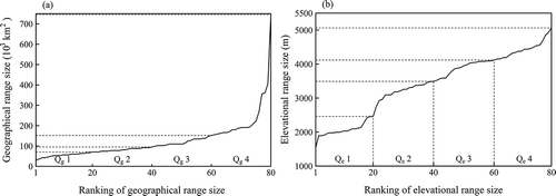
We then ranked the 80 species from the most narrow ranged to the most wide ranged, and partitioned the species over the four quartiles: small (Q_g1 and Q_e1), medium (Q_g2 and Q_e2), large (Q_g3 and Q_e3) and very large (Q_g4 and Q_e4) quartiles (20, 20, 20 and 20 species per quartile, respectively) for both geographical (Q_g) and elevational (Q_e) range sizes (Figure 2).

Figure 2. The geographical (a) and elevational (b) range sizes covered by the quartiles.

2.5. Statistical analyses

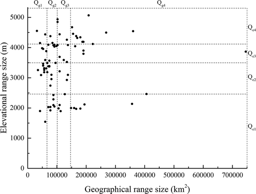
We used the non-parametric Spearman’s rank-order correlation to estimate the relationship between geographical and elevational range sizes, because the geographical range sizes had a very skewed distribution due to four species having a very large range size (over 3 × 10⁶ km², Figure 2(a)). We performed a non-parametric Mann-Whitney U test to examine whether the difference of model performance (AUC and TSS_max) was significant. We used variable contribution, a standard output of MaxEnt expressed as percentage, to estimate the importance of variables in explaining the distribution of the rhododendron species. Response curves, which are also part of the output from MaxEnt, were used to interpret how individual variables affect the probability of presence of rhododendron species belonging to the different quartiles of range sizes.

3. Results

3.1. Relationship between geographical and elevational range size

The correlation between geographical and elevational range sizes of rhododendron species was not significant (r = 0.17, P = 0.13; Figure 3), indicating that geographically narrow-ranged species do not necessarily also have a narrow range in elevation and vice versa. Thus elevational range size can be considered as another trait than geographical range size. In our further analyses, geographical and elevational range size groups will be analysed separately.

Figure 3. Correlation between geographical range size and elevational range size of rhododendron species.

3.2. Model performance of the four categories of environmental variables

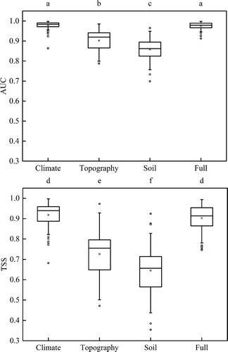
The fitted models based on climatic, topographic, edaphic and all (full) variables showed differences in prediction accuracies (Figure 4, P < 0.01). When comparing each model’s AUC and TSS for all 80 rhododendron species, the climatic and full models had significantly higher predictive accuracy than the topography and soil models. With a mean AUC value of 0.978 and TSS value of 0.919, the climate model had slightly higher absolute scores compared with the full model (AUC = 0.975, TSS = 0.903, model performance of 80 species see Appendix Table A1), but the difference was not significant.

Figure 4. Comparison of the prediction accuracy of four categorical environmental variables for the distribution of 80 rhododendron species in China. Different letters indicate significant differences (P < 0.01).

3.3. Importance of variables across geographical range sizes

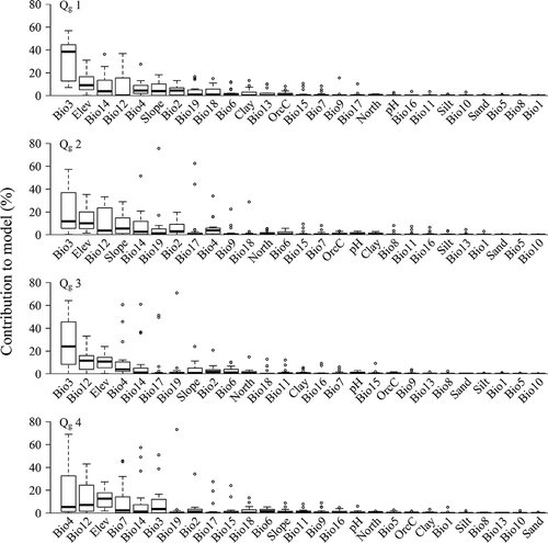
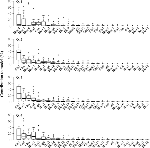
We considered the top five most explaining variables for further analysis, which in total explained between 60% and 70% of the distribution of species (Figure 5). The mean contribution of variables across all species within a range size groups is reported hereafter. The average importance of isothermality (Bio3; ~33%) for geographically narrow-ranged species (Q_g1) became gradually less for geographically wide-ranged species (~11%), while the average importance of seasonality (Bio4) and temperature annual range (Bio7) increased for the geographically wide-ranged species (~19% and 9%). Elevation and precipitation in the driest month (Bio14) had a similar importance across range sizes. The importance of annual precipitation (Bio12) also changed significantly across range sizes, only contributing ~2% for Q_g1, but up to 12% for the other three quartiles (Q_g2, Q_g3 and Q_g4). Slope was only important for the geographically narrow-ranged species.

Figure 5. Contributions of the 27 environmental variables sorted from highest to lowest across geographical range size groups (Q_g1–Q_g4, see Figure 2).

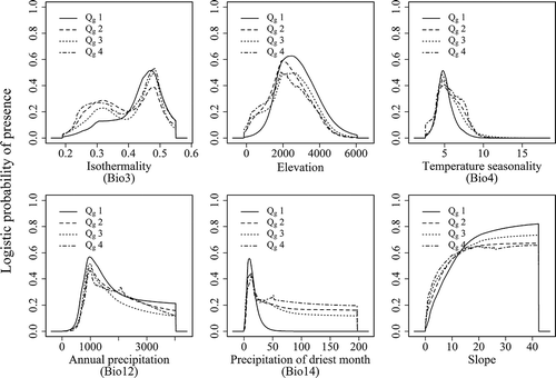
The responses of the important variables in the prediction for the four geographic range size groups as well as for each species were showed in Figure 6 and Figure A2, respectively. According to the response curves, the geographically narrow-ranged species (Q_g1) occurred in areas with less variation in the diurnal temperature range than in the annual temperature range (i.e. higher values for isothermality (Bio3) of about 0.4–0.55) compared with the other three quartiles (with ranges in Bio3 of 0.2–0.55). They also occurred in areas with a narrower range of temperature seasonality (Bio4 between 2.75 and 6). Precipitation in the driest month (Bio14) from 5 to 30 mm and a slope gradient of 15–40° would be favoured by Q_g1. In general, the geographically wide-ranged species (Q_g2–Q_g4) can be found over broader ranges of these conditions than the geographically narrow-ranged species (Q_g1).

Figure 6. Averaged response curves of the four geographical range size groups for the six most important environmental variables based on the full model.

3.4. Importance of variables across elevational range sizes

For the elevational range size groups (Figure 7), isothermality (Bio3) was significantly important (32%) for the middle-ranged species (Q_e2 and Q_e3). Ranked as the third important variable, elevation contributed around 10% for all four groups. Temperature seasonality (Bio4, ~17%) and annual temperature range (Bio7, ~8%) were more important for elevationally wide-ranged species (Q_e4), while precipitation in the driest month (Bio14, ~20%) and in the driest quarter (Bio17, ~14%), and the precipitation of the coldest quarter (Bio19, ~11%) were only important for species with a narrow elevational range (Q_e1).

Figure 7. Contributions of the 27 environmental variables, sorted from highest to lowest importance, across elevational range size groups (Q_e1–Q_e4, see Figure 2).

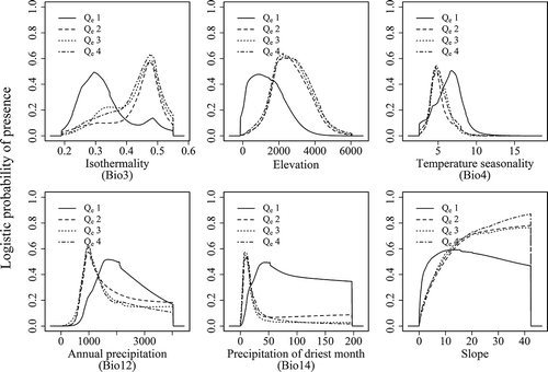
The responses of the important variables in the prediction for the four elevational range size groups as well as for each species were indicated in Figure 8 and Figure A3, respectively. The responses curves showed that the species with elevationally medium and wide range (Q_e2, Q_e3 and Q_e4) did not in fact tolerate a wider range of conditions than the narrow-ranged species. In general, narrow-ranged species (Q_e1) showed a shifted pattern compared to the other quartiles. For example, Isothermality (Bio3) played a primary role in all the groups (significantly important for Q_e2 and Q_e3), but the narrow-ranged species were generally found in areas with large variations in diurnal temperature relative to the annual temperature range (i.e. low values [0.2–0.35] of isothermality). Precipitation in the driest month (Bio14) was the most important factor for Q_e1. Narrow-ranged species occurred in areas where precipitation in the driest month (Bio14) was ≥20 mm (up to 200 mm), while the other three quartiles occurred in areas with up to 50 mm at most. Q_e1 also occurred in the temperature seasonality (Bio 4) range of 2–10°, while this range shrank to 2–8° for the medium- and wide-ranged groups.

Figure 8. Averaged response curves of the four elevational range size groups for the six most important environmental variables based on the full model.

4. Discussion

4.1. Climatic variables are more important as a measure of niche breadth at large spatial extents

Our results support earlier studies which concluded that climatic variables play an important role in shaping plant species’ range when they occur over large spatial extents or areas (Kockemann et al. 2009, Thomas 2010, Morin and Lechowicz 2013). Given our results show a consistently large importance of isothermality (Bio3) across all groups, and a substantial importance of temperature seasonality (Bio4) for the wide-ranged species, both geographically and elevationally, we would emphasize that climatic variables, and especially seasonal variation, should be included as a measure of the niche breadth that determines species’ distributional ranges over large areas. This is in line with Quintero and Wiens (2013) who concluded that seasonal variation explains most of the variation in climatic niche breadths among species.

Isothermality quantifies how much the diurnal (day-to-night) temperatures oscillate relative to the summer-to-winter (seasonal/annual) oscillations. Some biogeographical studies have noted coincidences between geographical range boundaries and temperature isotherms (Calosi et al. 2010). However, isothermality was often overlooked in studies that correlated environmental factors with species’ range sizes. This is most probably because isothermality is derived from annual mean diurnal range (Bio2) and annual temperature range (Bio7). It would, therefore, be excluded if a collinearity analysis was performed before any further analysis. In our study area, isothermality is strongly correlated with annual mean diurnal range (Bio2; r = 0.9) and precipitation seasonality (Bio15; r = 0.86), which, on the one hand, indicates that Bio2 and Bio15 are also important, but they did not exhibit a high importance because Bio3 took their places. On the other hand, it could be because the bioclimatic information in Bio3 is more relevant in explaining the distribution of rhododendrons. Temperature seasonality (Bio4) is a measure of temperature change during the year. Over a large area, seasonality indicates periodic departures from the climatic optima for organisms, so high seasonality favours species with adaptations to cope with unevenly distributed resources or conditions. In this sense, seasonality could be acting as an environmental filter for species distributional range (Gouveia et al. 2013). Because of the strong correlation between temperature seasonality (Bio4) and temperature annual range (Bio 7), we suspect that temperature annual range is potentially also important, particularly for the wide-ranged species. So, climatic variation is considered as a vital determinant for the distribution of alpine and subalpine plant species.

Conversely, although soil properties have been employed as important factors of niche breadth related to variation of geographical range size (Morin and Lechowicz 2013, Pannek et al. 2013), the minor importance of edaphic variables in the distribution of all range size groups of rhododendron species seen in our study does not provide any support for this. One possible explanation may lie in the issue of scale. The importance of explanatory variables for species with different range sizes depend both on grain and extent. Different processes determine geographical ranges as the spatial extent of the investigation changes (Baltzer et al. 2007, Slatyer et al. 2013). Climatic variables are the most important in determining species’ distribution on continental to global scales, whereas edaphic variables are more important at smaller scales (Pearson and Dawson 2003, Morin and Chuine 2006).

The topographic explanatory variables ranked as the second most important set of explanatory variables. Elevation is always among the top five most important variables across range size groups. We, therefore, infer that a combination of climate variables changing with elevation (Janzen 1967), and the influence of topography itself (as a barrier to dispersion) might lead to the relative importance of elevation. The moderate to strong correlations we found between topographic and climatic variables (Appendix Figure A1) can partly explain the secondary importance of elevation.

4.2. Climatic niche breadth determines variation in geographical range size

We found that the geographically wide-ranged species occurred across a broader range of climatic niche conditions, which suggests that species capable of enduring wide ranges of climate conditions can occupy larger geographical ranges. In other words, our results provide empirical support for the climatic variability hypothesis, which can be considered as a sub-hypothesis of the niche breadth hypothesis for explaining the variation in geographical range size of plant species. However, it is worth noting that a critical assumption in the climatic variability hypothesis is that there is indeed an appropriate gradient (latitudinal, altitudinal or otherwise) in climatic variability (Addo-Bediako et al. 2000). In most cases, geographical range size is an analogue of latitudinal gradients, and climate shows less variation at lower latitudes than higher latitudes within China. Our results therefore support the climatic variability hypothesis. Since this hypothesis was proposed by Stevens (1989), it has been confirmed by a number of studies. More recent studies have used the term ‘climatic niche breadth’ rather than ‘climatic variability’ to illustrate the ability (range) that can be tolerated by one species (Fisher-Reid et al. 2012, Köster et al. 2013, Arellano et al. 2014). Sheth et al. (2014) showed that climatic niche breadth, which is the range of climatic condition a species occurs in, explained more variation than the niche position, which is a species’ niche relative to the central tendency of climatic conditions in a study region for the geographical range size of monkeyflower species (genus Mimulus). Sheth and Angert (2014) also explained the positive strong relationship between the capacity of a species to cope with climatic variability and its geographical range size from an evolutionary viewpoint. They suggested that a species with a broader climate tolerance may be composed of phenotypically plastic genotypes. This would allow for stronger local adaptations by divergent subpopulations to their individual environments. Such species could also harbour greater genetic variation, allowing for a greater environmental tolerance.

Meanwhile, we have shown that variation in elevational range sizes can be mainly explained by shifts in niche range, rather than by differences in the width of these ranges. Precipitation in the driest month seems to be a crucial factor. Elevationally narrow-ranged species require more rainfall in the driest month than the other range size groups, suggesting that these species are more sensitive to drought conditions than wider-ranged species. A combination of orographically induced increases in precipitation with increasing elevation, and decreasing moisture availability at higher altitudes (due to shallower soils) might help create optimal conditions only at very specific elevations (Allamano et al. 2009, Quintero and Wiens 2013). In addition, although climatic variability was also proposed to explain the variation of elevational range size (Stevens 1992), it only applies when the climatic variability increases with elevational range. We thus speculate that there is no linear correlation between climatic niche breadth and elevation range in our study of rhododendron species in China. However, steep elevation-induced environmental gradients may limit the habitat available for a species and also act as dispersal barriers between similar environments, effectively restricting the range size (Morueta-Holme et al. 2013). In fact, variation of elevational range size has been paid little attention in the past years. This is partly due to the conclusion that variation of elevational range is only an extension of variation of geographical range (Stevens 1992). In addition, the relative few available studies focused on mountain systems and elevational gradients (see White and Bennett 2015). More taxa thus need to be tested to confirm if there is a more general pattern to be identified.

4.3. Differences between species with narrow geographical and elevational range sizes

The geographically narrow-ranged species occur where there are small variations in diurnal, seasonal and annual temperatures, and where small amounts of precipitation in the driest month can be expected. The elevationally narrow-ranged species occur where there are large variations in diurnal, seasonal and annual temperatures, and where there is still ample precipitation in the driest month. Possibly it is the elevationally narrow-ranged species that grow on the middle part of a mountain, where precipitation is ample and temperature variability is relatively high. The geographically narrow-ranged species could be mainly restricted to specific valleys where the temperatures are more stable. The very weak correlation between both types of range sizes and the distinctly different niche conditions, where narrow-ranged species of both groups occur, suggests that elevational range size can be seen as a complementary trait to geographical range size, containing different information on the environmental requirements of plants.

4.4. Implications of climate change

The high importance of isothermality (Bio3), temperature seasonality (Bio4) and precipitation in the driest month (Bio14) in the fitted models in this study suggests that changes of these three variables in the future would have the most profound effects on the distribution in alpine and subalpine plant species. This would especially be the case for species with narrow tolerance ranges. When we compared the current ranges and projections of two models, HadGEM2-ES and MIROC-ESM (available at: http://www.worldclim.org/cmip5_30s), isothermality was expected to stay constant but temperature seasonality and precipitation in the driest month were expected to decrease over the whole of China until 2070. This will affect both the geographically narrow- ranged species that have small tolerance ranges for these variables as well as the elevationally narrow-ranged species that require higher amounts of precipitation in the driest months. Geographically and elevationally wide-ranged species may be affected to only a limited extent by these changes.

Acknowledgments

This work of the first author was supported by the China Scholarship Council and co-funded by ITC Research Fund from the Faculty of Geo-Information Science and Earth Observation (ITC), University of Twente, the Netherlands. We are grateful to Dr Wenyun Zuo for her data-sharing initiative.

Disclosure statement

No potential conflict of interest was reported by the authors.

Additional information

Funding

This work was supported by the China Scholarship Council and co-funded by ITC Research Fund from the Faculty of Geo-Information Science and Earth Observation (ITC), University of Twente, the Netherlands.

Appendix

Figure A1. Correlation coefficients between variables. All the correlations were significant (P < 0.05). Correlations higher than 0.7 are given in bold with a grey background.

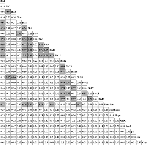
Figure A2. Response curves of each species in the four geographical range size groups.

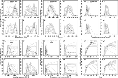
Figure A3. Response curves of each species in the four elevational range size groups.

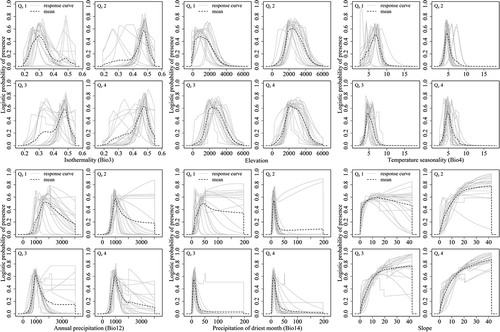
Table A1. Number of samples used for model training/evaluation and AUC and TSS of full model.

Species	Training samples	Test samples	AUC	TSS
Rhododendron aganniphum Balf.f.et K.Ward.	96	40	0.973	0.914
Rhododendron agastum Balf.f.et W.W.Smith	21	9	0.986	0.968
Rhododendron alutaceum Balf.f.et W.W.Smith	33	14	0.987	0.916
Rhododendron ambiguum Hemsl.	27	11	0.989	0.977
Rhododendron argyrophyllum	40	17	0.976	0.865
Rhododendron augustinii Hemsl.	101	43	0.960	0.841
Rhododendron auriculatum Hemsl.	26	11	0.963	0.865
Rhododendron bachii Lévl.	63	27	0.960	0.851
Rhododendron brevinerve Chun et Fang	28	12	0.981	0.884
Rhododendron bureavii Franch.	27	11	0.979	0.956
Rhododendron calophytum Franch.	55	23	0.989	0.954
Rhododendron calostrotum Balf.f.et K.ward	22	9	0.990	0.946
Rhododendron cavaleriei lévl	36	15	0.961	0.849
Rhododendron championae Hook	59	24	0.963	0.866
Rhododendron citriniflorum Balf.f.et Forrest	28	12	0.988	0.903
Rhododendron concinnum Hemsl.	70	30	0.968	0.904
Rhododendron coriaceum Franch.	21	9	0.997	0.991
Rhododendron davidsonianum Rehd.et Wils.	35	14	0.962	0.749
Rhododendron decorum Franch.	212	90	0.970	0.921
Rhododendron delavayi Franch.	114	48	0.976	0.906
Rhododendron discolor Franch.	47	20	0.958	0.833
Rhododendron eclecteum Balf.f.et Forrest	35	15	0.995	0.991
Rhododendron faberi Hemsl.subsp.faberi	29	12	0.991	0.962
Rhododendron farrerae Tate ex Sweet	26	10	0.972	0.929
Rhododendron floccigerum Franch	33	14	0.952	0.832
Rhododendron fortunei Lindl.	69	29	0.958	0.768
Rhododendron fulvum Balf.f.et.W.W.Smith	52	22	0.989	0.960
Rhododendron haematodes Franch.	42	17	0.995	0.985
Rhododendron heliolepis Franch.	89	37	0.970	0.935
Rhododendron henryi Hance	28	12	0.976	0.935
Rhododendron hippophaeoides Balf.f.et Forrest	42	18	0.978	0.891
Rhododendron hypoglaucum Hemsl.	22	9	0.978	0.877
Rhododendron irroratum Franch.	92	39	0.981	0.921
Rhododendron liliiflorum Lévl.	26	10	0.972	0.889
Rhododendron lukiangense Franch.	39	16	0.986	0.954
Rhododendron lutescens Franch.	55	23	0.979	0.926
Rhododendron maculiferum Franch.	29	12	0.939	0.810
Rhododendron mariae Hance	45	18	0.967	0.877
Rhododendron mariesii Hemsl.et Wils.	147	63	0.926	0.763
Rhododendron microphyton Franch.	60	25	0.986	0.957
Rhododendron molle (Blume) G.Don	31	13	0.927	0.757
Rhododendron neriiflorum Franch.	31	13	0.979	0.904
Rhododendron nivale Hook. f.	62	26	0.958	0.808
Rhododendron oreodoxa Franch.	48	20	0.959	0.790
Rhododendron ovatum (Lindl.) Planch.ex Maxim.	142	60	0.946	0.818
Rhododendron pachytrichum Franch.	28	11	0.989	0.941
Rhododendron phaeochrysum Balf.f.et W.W.Smith	92	39	0.975	0.891
Rhododendron polylepis Franch.	33	14	0.992	0.965
Rhododendron primuliflorum Bur.et Franch.	53	22	0.973	0.893
Rhododendron protistum Balf.f.et Forrest	21	9	0.998	0.993
Rhododendron racemosum Franch.	159	67	0.980	0.953
Rhododendron rex Lévl.	75	31	0.983	0.949
Rhododendron rivulare Hand.-Mazz.	43	18	0.967	0.807
Rhododendron roxieanum Forrest	46	19	0.975	0.865
Rhododendron rubiginosum Franch.	103	43	0.980	0.913
Rhododendron rupicola W. W.Smith	48	20	0.971	0.860
Rhododendron saluenense Franch.	46	19	0.980	0.911
Rhododendron sanguineum Franch.	47	20	0.984	0.944
Rhododendron scabrifolium Franch.	61	26	0.992	0.985
Rhododendron selense Franch.	45	19	0.990	0.948
Rhododendron seniavinii Maxim.	30	12	0.962	0.878
Rhododendron siderophyllum Franch.	73	31	0.953	0.821
Rhododendron simiarum Hance	63	27	0.965	0.836
Rhododendron simsii Planch.	316	135	0.913	0.746
Rhododendron sinonuttallii Balf.f.et Forrest	25	10	0.998	0.991
Rhododendron sperabiloides Tagg et Forrer	26	10	0.991	0.948
Rhododendron spiciferum Franch.	62	26	0.988	0.957
Rhododendron spinuliferum Franch.	98	42	0.987	0.934
Rhododendron stamineum Franch.	109	46	0.951	0.781
Rhododendron strigillosum Franch.	27	11	0.991	0.969
Rhododendron sutchuenense Franch.	29	12	0.970	0.893
Rhododendron tanastylum Balf.f.et K.Ward	36	15	0.983	0.914
Rhododendron tatsiense Franch.	56	24	0.991	0.952
Rhododendron telmateium Balf.f.et W.W.Smith	25	10	0.994	0.984
Rhododendron traillianum Forrest et W.W.Smith	35	15	0.995	0.988
Rhododendron trichostomum Franch.	41	17	0.970	0.913
Rhododendron triflorum Hook.f.	26	11	0.996	0.985
Rhododendron uvariifolium Diels	63	27	0.990	0.979
Rhododendron vernicosum Franch.	70	29	0.974	0.909
Rhododendron wardii W. W. Smith	58	24	0.988	0.944

References

- Addo-Bediako, A., Chown, S.L., and Gaston, K.J., 2000. Thermal tolerance, climatic variability and latitude. Proceedings of the Royal Society B-Biological Sciences, 267 (1445), 739–745. doi:10.1098/rspb.2000.1065
- Allamano, P., et al., 2009. A data-based assessment of the dependence of short-duration precipitation on elevation. Physics and Chemistry of the Earth, Parts A/B/C, 34 (10–12), 635–641. doi:10.1016/j.pce.2009.01.001
- Allouche, O., Tsoar, A., and Kadmon, R., 2006. Assessing the accuracy of species distribution models: prevalence, kappa and the true skill statistic (TSS). Journal of Applied Ecology, 43 (6), 1223–1232. doi:10.1111/jpe.2006.43.issue-6
- Anderson, R.P. and Gonzalez, I., 2011. Species-specific tuning increases robustness to sampling bias in models of species distributions: an implementation with Maxent. Ecological Modelling, 222 (15), 2796–2811. doi:10.1016/j.ecolmodel.2011.04.011
- Arellano, G., Cala, V., and Macia, M.J., 2014. Niche breadth of oligarchic species in Amazonian and Andean rain forests. Journal of Vegetation Science, 25 (6), 1355–1366. doi:10.1111/jvs.12180
- Baltzer, J.L., et al., 2007. Geographical distributions in tropical trees: can geographical range predict performance and habitat association in co-occurring tree species? Journal of Biogeography, 34 (11), 1916–1926. doi:10.1111/j.1365-2699.2007.01739.x
- Blackburn, T.M. and Ruggiero, A., 2001. Latitude, elevation and body mass variation in Andean passerine birds. Global Ecology and Biogeography, 10 (3), 245–259. doi:10.1046/j.1466-822X.2001.00237.x
- Botts, E.A., Erasmus, B.F.N., and Alexander, G.J., 2013. Small range size and narrow niche breadth predict range contractions in South African frogs. Global Ecology and Biogeography, 22 (5), 567–576. doi:10.1111/geb.12027
- Boulangeat, I., et al., 2012. Niche breadth, rarity and ecological characteristics within a regional flora spanning large environmental gradients. Journal of Biogeography, 39 (1), 204–214. doi:10.1111/j.1365-2699.2011.02581.x
- Brown, J.H., 1984. On the relationship between abundance and distribution of species. The American Naturalist, 124 (2), 255–279. doi:10.1086/284267
- Brown, J.H., Stevens, G.C., and Kaufman, D.M., 1996. The geographic range: size, shape, boundaries, and internal structure. Annual Review of Ecology and Systematics, 27, 597–623. doi:10.1146/annurev.ecolsys.27.1.597
- Calosi, P., et al., 2010. What determines a species’ geographical range? Thermal biology and latitudinal range size relationships in European diving beetles (Coleoptera: Dytiscidae). Journal of Animal Ecology, 79 (1), 194–204. doi:10.1111/j.1365-2656.2009.01611.x
- Chen, I.C., et al., 2011. Rapid range shifts of species associated with high levels of climate warming. Science, 333 (6045), 1024–1026. doi:10.1126/science.1206432
- Devictor, V., et al., 2010. Defining and measuring ecological specialization. Journal of Applied Ecology, 47 (1), 15–25. doi:10.1111/j.1365-2664.2009.01744.x
- Elith, J., et al., 2011. A statistical explanation of MaxEnt for ecologists. Diversity and Distributions, 17 (1), 43–57. doi:10.1111/j.1472-4642.2010.00725.x
- Fielding, A.H. and Bell, J.F., 1997. A review of methods for the assessment of prediction errors in conservation presence/absence models. Environmental Conservation, 24 (1), 38–49. doi:10.1017/S0376892997000088
- Fisher-Reid, M.C., Kozak, K.H., and Wiens, J.J., 2012. How is the rate of climatic-niche evolution related to climatic-niche breadth? Evolution, 66 (12), 3836–3851. doi:10.1111/evo.2012.66.issue-12
- Gaston, K.J., 1996. Species-range-size distributions: patterns, mechanisms and implications. Trends in Ecology & Evolution, 11 (5), 197–201. doi:10.1016/0169-5347(96)10027-6
- Gaston, K.J., Blackburn, T.M., and Lawton, J.H., 1997. Interspecific abundance range size relationships: an appraisal of mechanisms. The Journal of Animal Ecology, 66 (4), 579–601. doi:10.2307/5951
- Gaston, K.J. and Spicer, J.I., 2001. The relationship between range size and niche breadth: a test using five species of Gammarus (Amphipoda). Global Ecology and Biogeography, 10 (2), 179–188. doi:10.1046/j.1466-822x.2001.00225.x
- Ghalambor, C.K., et al., 2006. Are mountain passes higher in the tropics? Janzen’s hypothesis revisited. Integrative and Comparative Biology, 46 (1), 5–17. doi:10.1093/icb/icj003
- Gouveia, S.F., et al., 2013. Nonstationary effects of productivity, seasonality, and historical climate changes on global amphibian diversity. Ecography, 36 (1), 104–113. doi:10.1111/j.1600-0587.2012.07553.x
- Hengl, T., et al., 2014. SoilGrids1km–global soil information based on automated mapping. Plos One, 9 (8), e105992. doi:10.1371/journal.pone.0105992
- Hijmans, R.J., et al., 2005. Very high resolution interpolated climate surfaces for global land areas. International Journal of Climatology, 25 (15), 1965–1978. doi:10.1002/joc.1276
- Jansson, R., 2003. Global patterns in endemism explained by past climatic change. Proceedings of the Royal Society B-Biological Sciences, 270 (1515), 583–590. doi:10.1098/rspb.2002.2283
- Janzen, D.H., 1967. Why mountain passes are higher in the tropics. The American Naturalist, 101 (919), 233–249. doi:10.1086/282487
- Jiang, Y., et al., 2014. Satellite-derived vegetation indices contribute significantly to the prediction of epiphyllous liverworts. Ecological Indicators, 38, 72–80. doi:10.1016/j.ecolind.2013.10.024
- Jobbagy, E.G. and Jackson, R.B., 2000. The vertical distribution of soil organic carbon and its relation to climate and vegetation. Ecological Applications, 10 (2), 423–436. doi:10.1890/1051-0761(2000)010[0423:TVDOSO]2.0.CO;2
- Kockemann, B., Buschmann, H., and Leuschner, C., 2009. The relationships between abundance, range size and niche breadth in Central European tree species. Journal of Biogeography, 36 (5), 854–864. doi:10.1111/j.1365-2699.2008.02022.x
- Köster, N., et al., 2013. Range size and climatic niche correlate with the vulnerability of epiphytes to human land use in the tropics. Journal of Biogeography, 40 (5), 963–976. doi:10.1111/jbi.2013.40.issue-5
- Kreyling, J., et al., 2015. Cold tolerance of tree species is related to the climate of their native ranges. Journal of Biogeography, 42 (1), 156–166.
- Kumar, P., 2012. Assessment of impact of climate change on Rhododendrons in Sikkim Himalayas using Maxent modelling: limitations and challenges. Biodiversity and Conservation, 21 (5), 1251–1266. doi:10.1007/s10531-012-0279-1
- Lenoir, J. and Svenning, J.C., 2015. Climate-related range shifts - a global multidimensional synthesis and new research directions. Ecography, 38 (1), 15–28. doi:10.1111/ecog.00967
- Li, Z., et al., 2013. The growth-ring variations of alpine shrub Rhododendron przewalskii reflect regional climate signals in the alpine environment of Miyaluo Town in Western Sichuan Province, China. Acta Ecologica Sinica, 33 (1), 23–31. doi:10.1016/j.chnaes.2012.12.004
- Liang, E.Y. and Eckstein, D., 2009. Dendrochronological potential of the alpine shrub Rhododendron nivale on the south-eastern Tibetan Plateau. Annals of Botany, 104 (4), 665–670. doi:10.1093/aob/mcp158
- Liu, C., et al., 2013. Selecting thresholds for the prediction of species occurrence with presence-only data. Journal of Biogeography, 40 (4), 778–789. doi:10.1111/jbi.12058
- Lowry, E. and Lester, S.E., 2006. The biogeography of plant reproduction: potential determinants of species’ range sizes. Journal of Biogeography, 33 (11), 1975–1982. doi:10.1111/jbi.2006.33.issue-11
- Ma, Y., et al., 2014. The conservation of Rhododendrons is of greater urgency than has been previously acknowledged in China. Biodiversity and Conservation, 23 (12), 3149–3154. doi:10.1007/s10531-014-0764-9
- McCain, C.M., 2006. Do elevational range size, abundance, and body size patterns mirror those documented for geographic ranges? A case study using Costa Rican rodents. Evolutionary Ecology Research, 8 (3), 435–454.
- McCauley, S.J., et al., 2014. Dispersal, niche breadth and population extinction: colonization ratios predict range size in North American dragonflies. Journal of Animal Ecology, 83 (4), 858–865. doi:10.1111/1365-2656.12181
- Morin, X. and Chuine, I., 2006. Niche breadth, competitive strength and range size of tree species: a trade-off based framework to understand species distribution. Ecology Letters, 9 (2), 185–195. doi:10.1111/j.1461-0248.2005.00864.x
- Morin, X. and Lechowicz, M.J., 2013. Niche breadth and range area in North American trees. Ecography, 36 (3), 300–312. doi:10.1111/j.1600-0587.2012.07340.x
- Morueta-Holme, N., et al., 2013. Habitat area and climate stability determine geographical variation in plant species range sizes. Ecology Letters, 16 (12), 1446–1454. doi:10.1111/ele.12184
- Munns, R., 2002. Comparative physiology of salt and water stress. Plant Cell and Environment, 25 (2), 239–250. doi:10.1046/j.0016-8025.2001.00808.x
- Ohlemuller, R., et al., 2008. The coincidence of climatic and species rarity: high risk to small-range species from climate change. Biology Letters, 4 (5), 568–572. doi:10.1098/rsbl.2008.0097
- Olalla-Tarraga, M.A., et al., 2011. Climatic niche conservatism and the evolutionary dynamics in species range boundaries: global congruence across mammals and amphibians. Journal of Biogeography, 38 (12), 2237–2247. doi:10.1111/j.1365-2699.2011.02570.x
- Pannek, A., Ewald, J., and Diekmann, M., 2013. Resource-based determinants of range sizes of forest vascular plants in Germany. Global Ecology and Biogeography, 22 (8), 1019–1028. doi:10.1111/geb.12055
- Parmesan, C., 2006. Ecological and evolutionary responses to recent climate change. Annual Review of Ecology Evolution and Systematics, 37, 637–669. doi:10.1146/annurev.ecolsys.37.091305.110100
- Pearson, R.G. and Dawson, T.P., 2003. Predicting the impacts of climate change on the distribution of species: are bioclimate envelope models useful? Global Ecology and Biogeography, 12 (5), 361–371. doi:10.1046/j.1466-822X.2003.00042.x
- Pérez-García, N., et al., 2013. Drastic reduction in the potential habitats for alpine and subalpine vegetation in the Pyrenees due to twenty-first-century climate change. Regional Environmental Change, 13 (6), 1157–1169. doi:10.1007/s10113-013-0427-5
- Phillips, S.J., Anderson, R.P., and Schapire, R.E., 2006. Maximum entropy modeling of species geographic distributions. Ecological Modelling, 190 (3–4), 231–259. doi:10.1016/j.ecolmodel.2005.03.026
- Phillips, S.J. and Dudik, M., 2008. Modeling of species distributions with Maxent: new extensions and a comprehensive evaluation. Ecography, 31 (2), 161–175. doi:10.1111/j.0906-7590.2008.5203.x
- Pither, J., 2003. Climate tolerance and interspecific variation in geographic range size. Proceedings of the Royal Society B-Biological Sciences, 270 (1514), 475–481. doi:10.1098/rspb.2002.2275
- Prates-Clark, C.D.C., Saatchi, S.S., and Agosti, D., 2008. Predicting geographical distribution models of high-value timber trees in the Amazon Basin using remotely sensed data. Ecological Modelling, 211 (3–4), 309–323. doi:10.1016/j.ecolmodel.2007.09.024
- Purvis, A., et al., 2000. Predicting extinction risk in declining species. Proceedings of the Royal Society B-Biological Sciences, 267 (1456), 1947–1952. doi:10.1098/rspb.2000.1234
- Quintero, I. and Wiens, J.J., 2013. What determines the climatic niche width of species? The role of spatial and temporal climatic variation in three vertebrate clades. Global Ecology and Biogeography, 22 (4), 422–432. doi:10.1111/geb.12001
- Sheth, S.N. and Angert, A.L., 2014. The evolution of environmental tolerance and range size: a comparison of geographically restricted and widespread Mimulus. Evolution, 68 (10), 2917–2931. doi:10.1111/evo.12494
- Sheth, S.N., Jimenez, I., and Angert, A.L., 2014. Identifying the paths leading to variation in geographical range size in western North American monkeyflowers. Journal of Biogeography, 41 (12), 2344–2356. doi:10.1111/jbi.12378
- Slatyer, R.A., Hirst, M., and Sexton, J.P., 2013. Niche breadth predicts geographical range size: a general ecological pattern. Ecology Letters, 16 (8), 1104–1114. doi:10.1111/ele.12140
- Stevens, G.C., 1989. The latitudinal gradient in geographical range: how so many species coexist in the tropics. The American Naturalist, 133 (2), 240–256. doi:10.1086/284913
- Stevens, G.C., 1992. The elevational gradient in altitudinal range: an extension of Rapoport’s latitudinal rule to altitude. The American Naturalist, 140 (6), 893–911. doi:10.1086/285447
- Theurillat, J.P. and Guisan, A., 2001. Potential impact of climate change on vegetation in the European Alps: a review. Climatic Change, 50 (1–2), 77–109. doi:10.1023/A:1010632015572
- Thomas, C.D., 2010. Climate, climate change and range boundaries. Diversity and Distributions, 16 (3), 488–495. doi:10.1111/j.1472-4642.2010.00642.x
- Thomas, C.D., et al., 2001. Ecological and evolutionary processes at expanding range margins. Nature, 411 (6837), 577–581. doi:10.1038/35079066
- Thomas, C.D., et al., 2004. Extinction risk from climate change. Nature, 427 (6970), 145–148. doi:10.1038/nature02121
- Thompson, K., Gaston, K.J., and Band, S.R., 1999. Range size, dispersal and niche breadth in the herbaceous flora of central England. Journal of Ecology, 87 (1), 150–155. doi:10.1046/j.1365-2745.1999.00334.x
- Thuiller, W., Lavorel, S., and Araujo, M.B., 2005. Niche properties and geographical extent as predictors of species sensitivity to climate change. Global Ecology and Biogeography, 14 (4), 347–357. doi:10.1111/geb.2005.14.issue-4
- Wang, Z., et al., 2012. Geographical patterns in the beta diversity of China’s woody plants: the influence of space, environment and range size. Ecography, 35, 1092–1102. doi:10.1111/j.1600-0587.2012.06988.x
- White, R.L. and Bennett, P.M., 2015. Elevational distribution and extinction risk in birds. Plos One, 10 (4), e0121849. doi:10.1371/journal.pone.0121849
- Williams, J.N., et al., 2009. Using species distribution models to predict new occurrences for rare plants. Diversity and Distributions, 15 (4), 565–576. doi:10.1111/j.1472-4642.2009.00567.x
- Wisz, M.S., et al., 2008. Effects of sample size on the performance of species distribution models. Diversity and Distributions, 14 (5), 763–773. doi:10.1111/j.1472-4642.2008.00482.x