Vehicle trajectory modelling with consideration of distant neighbouring dependencies for destination prediction

ABSTRACT

Vehicle trajectory modelling is an essential foundation for urban intelligent services. In this paper, a novel method, Distant Neighbouring Dependencies (DND) model, has been proposed to transform vehicle trajectories into fixed-length vectors which are then applied to predict the final destination. This paper defines the problem of neighbouring and distant dependencies for the first time, and then puts forward a way to learn and memorize these two kinds of dependencies. Next, a destination prediction model is given based on the DND model. Finally, the proposed method is tested on real taxi trajectory datasets. Results show that our method can capture neighbouring and distant dependencies, and achieves a mean error of 1.08 km, which outperforms other existing models in destination prediction significantly.

KEYWORDS:

• Neighbouring and distant dependencies
• final destination prediction
• trajectory modelling
• Trajectory Node Vector
• Trajectory Sequence Vector

1. Introduction

With the rapid development of the urban road traffic system, road traffic monitoring and predicting play an essential role in urban traffic management (Besse et al. 2018). In recent years, the dramatically increased mobile devices, such as portable GPS devices, and smartphones have led to unexpected growth in vehicle trajectory data (Magdy et al. 2015). Trajectory modelling and destination prediction is vital to not only city traffic monitoring but also a lot of exciting applications, such as intelligent travelling schedule (Lv et al. 2018), targeted advertising based on destination and location-based social networking (Xue et al. 2013) and optimized scheduling strategies that reduce travel costs and energy consumptions.

The next location prediction of a trajectory is strongly influenced by recently visited locations (Liu et al. 2016, Yao et al. 2017). Similarly, to predict a trajectory’s final destination is also strongly related to current adjacent locations (Besse et al. 2018). Differently, the destination is also closely related to locations visited earlier, for instance, locations near the starting position. There is also a strong correlation between these distant locations. Wu et al. (2017) have mentioned that long-term dependencies existing among trajectory points are essential for trajectory modelling. Long-term dependencies that are usually related to user intents mean the co-occurring probability of locations that are far apart from each other on the same trajectory. Correspondingly, the co-occurring probability of adjacent locations reflects local movement characteristics. It is mainly affected by road topological constraints. We define these two kinds of dependencies as neighbouring dependencies and distant dependencies which together represent the movement characteristics. Most of the existing methods pay little attention to these two kinds of dependencies in trajectory modelling, but they are essential in reflecting spatial characteristics of the trajectory from both microscopic and macroscopic perspectives. If neighbouring dependencies were ignored, the prediction results would be inconsistent with the road structure. If distant dependencies were ignored, the prediction results might not get the real travel intents.

In this paper, we have proposed a three-step embedding method to model both neighbouring and distant dependencies. The first step is the neighbouring dependencies embedding. Seeing a trajectory as a sequence composed of road junctions (hereafter referred to as trajectory nodes), we apply the skip-gram model to learn neighbouring dependencies from adjacent nodes based on a sliding window. Then, each node is turned into a unique fixed-length vector, TNV. The second step is the sequence reconstruction, which replaces the trajectory nodes with the embeddings obtained in the first step to reconstruct the entire trajectory sequence. The third step is distant dependencies embedding. An LSTM neural network is used to model the reconstructed sequences. Then, an original trajectory can be transformed into a fixed-length vector, TSV. To predict destination by TSV, we connect a simple three-layer Neural Network which produces probabilities of control points. Then, the destination coordinates can be estimated through the expectation of positions of control points.

Moreover, we demonstrate how to apply this method to predict the final destinations of taxi trips on real datasets from ECML-PKDD contests.¹ The results reveal that our method performs much better than existing approaches to the best of our knowledge. Finally, in further experiments, we evaluate the geographical meaning of the two types of embedding vectors, TNV and TSV, produced by this method.

In summary, we make the following contributions in this work:

• To the best of our knowledge, this is the first time to capture neighbouring and distant dependencies simultaneously in trajectory modelling for improving destination prediction performance.

• We present a novel model, DND, that predicts destination based on partial trajectory and outperforms the state-of-the-art models by getting a mean error of 1.08 km in our experiments.

• We model neighbouring dependencies into Trajectory Node Vector (TNV) and find that TNV can learn the latent geographical regularities from historical trajectories. Our experiments prove that the geographical proximity and the topological proximity on the road network can be represented as the cosine distance between two TNVs.

• We use the DND model to encode a trajectory into a fixed-length vector, Trajectory Sequence Vector (TSV), from a GPS coordinate sequence. We find that TSV can learn not only the latent geographical regularities but also the user preferences. The clustering experiments reveal that the TNV can represent distant dependencies and road selection patterns.

The rest of this paper is organized as follows: Section 2 reviews related work. Section 3 illustrates the workflow of the proposed model. In Section 4, we introduce the experiments, compare our model with existing models, and further discuss the practical meaning of TNV and TSV. Finally, we draw conclusions and give our future works in Section 5.

2. Related work

Predicting the location of final destination based on a trajectory’s current locations usually involves three parts including trajectory pre-processing, trajectory representation modelling and destination prediction methods. In this section, we briefly review the related works to provide a background of the commonly used methods.

2.1 Trajectory pre-processing

A real vehicle trajectory describes object movement as a continuous spatial curve. However, stored trajectory data only record a discrete location sequence due to the limit of sensing device like GPS (Xie et al. 2017). Trajectory pre-processing is usually used to address two challenges introduced by the sampling uncertainty of raw GPS data when modelling trajectories for destination prediction. (1) The varying-length sequences of GPS points are incompatible with most machine learning methods. (2) The sparsity problem (Besse et al. 2018), which means GPS location points recorded at several observation times on the same road may completely different (Furtado et al. 2018), severely reduces prediction accuracy. To solve the varying-length problem, de Brébisson et al. (2015) and Lam et al. (2015) have proposed similar methods of selecting a fixed number of points from the original trajectories. For the sparsity problem, most solutions are inclined to resample original trajectories as segments collections (Tanaka et al. 2009, Xue et al. 2013, Wu et al. 2017), spatial discrete grids (Krumm and Horvitz 2006, Zhang et al. 2016, Wang et al. 2017, Lv et al. 2018) and categorized location labels (Xiao et al. 2010, Ying et al. 2011, Zhou et al. 2016) to raise the sampling density at the same position. Guo et al. (2018) perform an initial spatial clustering of points to cut down unnecessary data details and to speed up the computation. Bogorny et al. (2009) use external geographical information to represent the trajectory as a series of semantic tags and designed a data mining query language (ST-DMQL) to retrieve trajectories that contain specific semantics and calculate trajectory similarities. Among these works, few pre-processing methods devote to solving both the two problems at the same time.

2.2 Trajectory representation models

Trajectories aim to the same destinations can have similar moving patterns. In order to study user moving pattern and user intention, it is necessary to represent the trajectory in another form for mathematical calculations and other analytical models. Zhou et al. (2016) mention that the strong local correlation of sequence nodes contains context features of trajectory data, which is of great significance in trajectory modelling and representation. In order to make rational predictions, vehicle movement context should be taken into account in the trajectory representation models (Yao et al. 2017). In the field of natural language processing, the primary meaning of the distribution hypothesis (Harris 1954, Firth 1957) is that context-similar words have similar semantics. The word representation (Turian et al. 2010) stores information distributed in each dimension of a vector which is usually generated by neural network models. Inspired by this, researchers have introduced word embeddings into the trajectory modelling process. For example, Gao et al. (2017) use the word representation approach to obtain the low-dimensional vectors of location points of check-in trajectories, thereby mining the link relationship among users. Fan et al. (2018) use continuous vectors to retrieve context features among locations. Wu et al. (2017) treat a trajectory as a sequence of transition state from one edge to another and transform each state into an embedding vector to get dense representations of sequence units. Yao et al. (2018) extract a set of moving behaviour features with a fixed-length sliding window and then learn a fixed-length representation of a trajectory through a sequence-to-sequence model. Although these methods can model different movement characteristics in trajectories, it remains a challenge to transform trajectories into low-dimensional representations simultaneously retaining dependencies between visited locations that can cover a long distance or a short distance.

2.3 Destination prediction methods

Probabilistic approaches are widely adopted for trajectory prediction. Some researchers conduct early research on these methods (Krumm and Horvitz 2006, Ziebart et al. 2008b). They transform the trajectory prediction into probability distribution by the Bayesian model. After that, much work utilizes the Markov model and Bayesian Inference for destination prediction based on partial trajectories (Ziebart et al. 2008a, Xue et al. 2013, Zhang et al. 2016). Unfortunately, low-order Markov chains can only express local transition probabilities, and they cannot handle long-sequence dependencies. Besse et al. (2018) predict trajectories by classifying points of prefixes into clusters of historical trajectories through a mixture of Gaussian distributions. This method models trajectories at a relatively more macro scale, which provides a better understanding of car drivers’ behaviours. However, these probabilistic approaches are still too shallow to catch relations between two distant locations, which we call distant dependencies in this paper.

Some other works try to apply machine learning to destination prediction based on partial trajectories. For instance, tree-based models are utilized in this issue (Ying et al. 2011, Hoch 2015, Lam et al. 2015). Among them, Ying et al. (2011) model a trajectory as a sequence of position category tags and use an SPF-TREE to predict the next step of trajectory prefixes. Lam et al. (2015) cut out part of GPS coordinates from the original trajectory and predict corresponding final destination and travel time by Gradient Boosted Regression Trees, whose process can be accelerated by geohash. These methods encounter the sparsity problem in varying degrees. Indeed, it is difficult to improve the prediction accuracy of the destinations through tree-based models, as the coordinates of the destinations are continuous variables in geographic space. de Brébisson et al. (2015) first use deep learning methods in destination prediction by taking 5 points separately from the head and tail of the original sequence. This work also compares the performances of MLP, RNN, Bidirectional-RNN and Memory network model in destination prediction. Similarly, Liu et al. (2016) introduce the Temporal Context in this subject and implement the Spatial-Temporal prediction through RNN. Lv et al. (2018) model the trajectory as an image by discretizing the study area as a two-dimensional matrix composed of grids, and then predict the destination by training a CNN model. Wu et al. (2017) propose a trajectory model based on transition states and externally introduce road network topological constraints to improve training speed and accuracy. These methods can learn distant dependencies from different levels but can hardly learn dependencies between adjacent locations, because they mostly ignore learning associations between neighbouring locations. These dependencies are called neighbouring dependencies in this paper.

In general, most existing methods can capture moving characteristics of trajectories from large or small scales for destination prediction, but they can hardly model trajectories as fixed-length dense representations simultaneously retaining dependencies between visited locations that can cover a long distance or a short distance. Additionally, the prediction accuracy is limited by the model’s representative capability, which is not only related to the micro-features but also the macro-features of the entire trajectory. Therefore, jointly modelling neighbouring dependencies and distant dependencies is meaningful in trajectory prediction applications.

3. Trajectory modelling

In this section, a distant neighbouring dependencies (DND) model is introduced. Figure 1 shows the workflow of the DND model.

Figure 1. Workflow of the DND model.

The entire workflow is mainly composed of four parts.

• The first part is trajectory normalizing which transforms a trajectory into trajectory node sequence based on road junctions. (Section 3.1)

• The second part is neighbouring dependencies learning which discusses how to learn dependencies in neighbouring nodes and represents each node as a vector. (Section 3.2)

• The third part is distant dependencies learning which discusses how to learn dependencies in distant nodes and represents each sequence as a vector. (Section 3.3)

• The last part is about how to use DND model to predict final destinations based on the trajectory prefixes. (Section 3.4)

Definition 1 (Original Trajectory). An original trajectory $T$ is defined as $T=\{p_i\}$, where $p_i\in R^2$, $i\in [1,k]$, $p_i=(longitude,latitude)$ and $k$ is the length of sequence $T$. It represents the movements from one coordinate $p_1$ to another coordinate $p_2$ and so on to $p_k$ in the geographic space.

Definition 2 (Road Network). A road network, in this paper, is modelled as a directed graph $G(V,E)$, where $V$ means the set of vertices (road junctions) and $E$ means the set of edges. Each edge $e\in E$ represents a road segment from a vertex $v\in V$ to another vertex $v^{\prime }\in V$ and $v\ne v^{\prime }$.

3.1 Trajectory normalizing

To overcome the sparsity problem, we put forward a trajectory normalizing method. This method reduces the impact of sample uncertainty by converting a GPS coordinate sequence into a road junction sequence along its driving direction. In nature, this normalizing process maps a trajectory from the geographic space to the road network space and eliminates the uncertainty of location sampling. Consequently, the original trajectory is turned into a road junction sequence.

Definition 3 (Normalized Trajectory). A normalized trajectory $T^{\prime }$ is defined as $T^{\prime }=\{{\vartheta }_j\}$, where $j\in [1,n]$, ${\vartheta }_j\in V$, ${\vartheta }_j$ is defined as trajectory node, and $n$ is the length of $T^{\prime }$. Here, $n$ is usually smaller than $k$. In addition, $\mathrm{\forall }v\in V$ has at least 3 degrees on Road Network because the choice of next road segment on each ${\vartheta }_j\in V$ having less than 3 degrees is uniquely determined. It can reduce the computational complexity by reducing numbers of trajectory nodes.

As is shown in Figure 1, the normalizing process contains three main steps: (1) trajectory cleaning, (2) map matching and (3) junction sequence extracting. After trajectory cleaning, the error data caused by data loss, sampling drifting and some other abnormal sampling would be removed according to predefined driving rules. Then, the original GPS coordinates can be snapped to the road network by map matching using the Hidden Markov Chain method (Newson and Krumm 2009). Finally, we extract road junctions where the trajectory passed along the moving direction, and we also obtain a sequence consisting of trajectory nodes.

3.2 Neighbouring dependencies learning

A Random combination of trajectory nodes may not form a valid path due to the local road connectivity. The adjacent nodes in trajectories imply their connectivity on the road and preferences for road choice in local geographic space. We call this relationship neighbouring dependencies. Figure 2 shows that geographic locations have different interdependencies due to the different accessibility of road network. From common sense, dependency strength between neighbouring nodes mainly relies on road network topological constraints, and it is relatively stable. Instead of manually appending external information, we use a skip-gram model (Mikolov et al. 2013) to learn neighbouring dependencies automatically from historical trajectories.

Figure 2. Dependencies strength between neighbouring nodes. If someone needs to go from A to X, he must first go through B or C. From the perspective of graph theory, the cost from A to X is 2 degrees and the cost from B to X is 1 degree. It reflects that the dependencies strength between B and X is stronger than A and X.

The goal of neighbouring dependencies learning is to learn the weights of the hidden layer from the model, which can be trained to estimate neighbouring nodes according to the centre node in a window. Here, we define the objective function as:

(1) $\left(\omega \right)=\underset{(\omega )}{\text{arg}\text{max}}\frac{1}{n}{\displaystyle \sum _{j=1}^n{\displaystyle \sum _{-t\le l\le t,l\ne 0}logp\left({\vartheta }_{j+l}|{\vartheta }_j\right),}}$(1)

where ${\vartheta }_j$ denotes the centre node of a window size of $2t+1$, the neighbouring nodes of ${\vartheta }_j$ are ${\vartheta }_{j-t},...,{\vartheta }_{j-1},{\vartheta }_{j+1},...,{\vartheta }_{j+t}$. Then, the model uses a softmax to turn the output into classification probabilities. As a result, every trajectory node is transformed from a location point into a fixed-length vector.

Definition 4 (Trajectory Node Vector, TNV). A Trajectory Node Vector $v_j$, corresponding to ${\vartheta }_j$, is a d-dimension vector which comes from the hidden layer weights of the skip-gram model.

3.3 Distant dependencies learning

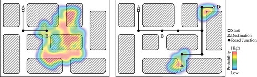
In addition to neighbouring dependencies, the factors that determine the macro characteristics of trajectory geometry are related to more abstract features such as travel purpose, driving preference, and even road traffic conditions. We call them distant dependencies because they are generally revealed by spatial co-occurrences among nodes that are relatively far apart from each other in historical trajectories. Taking the travel purpose as an example, stronger distant dependencies reflect more ascertainable destination. Since different trajectories may have same path portion, it is more difficult to estimate an accurate probability distribution of final destination if prefixes are short, like the path from A to B in Figure 3. However, if the trajectory passes C or D, the probability distribution will be concentrated in the geographic region because of stronger distant dependencies.

Figure 3. Distant dependencies influence the destination distribution.

Based on the above considerations, we design the framework of our model as five parts, (1) inputting trajectory nodes, (2) reconstructing a new trajectory sequence by replacing each trajectory node with its TNV, (3) learning distant dependencies by using a LSTM neural network, (4) outputting TSV, (5) learning task, as shown in Figure 4. The TNV sequence is used as input to ensure the model can capture enough neighbouring dependencies. In theory, learning tasks can be different machine learning models of trajectory mining, such as travel time estimation, next step prediction, behaviour mining, and so on. In this paper, the learning task is destination prediction.

Figure 4. Framework of the DND model.

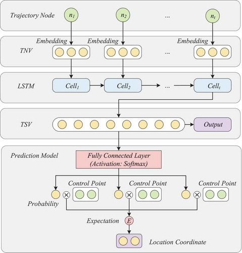
In this model, Long Short-term Memory (Hochreiter and Schmidhuber 1997) is used as a trajectory encoder to learn and embed distant dependencies into vector-based representations. Finally, we can get a fixed-length vector, TSV, for a trajectory through this encoder model. Equations (2) to (7) cover the main content of the LSTM neural network.

(2) ${\mathrm{\Gamma }}_f^{(t)}=\sigma (W_f[h^{(t-1)},x^{(t)}]+b_f)$(2)

(3) ${\mathrm{\Gamma }}_u^{(t)}=\sigma (W_u[h^{(t-1)},x^{(t)}]+b_u)$(3)

(4) ${\hat{c}}^{(t)}=tanh(W_c[h^{(t-1)},x^{(t)}]+b_c)$(4)

(5) $c^{(t)}={\mathrm{\Gamma }}_f^{(t)}\ast c^{(t-1)}+{\mathrm{\Gamma }}_u^{(t)}\ast {\hat{c}}^{(t)}$(5)

(6) ${\mathrm{\Gamma }}_o^{(t)}=\sigma (W_o[h^{(t-1)},x^{(t)}]+b_o)$(6)

(7) $h^{(t)}={\mathrm{\Gamma }}_o^{(t)}\ast tanh(c^{(t)}),$(7)

where ${\mathrm{\Gamma }}_f^{(t)}$, ${\mathrm{\Gamma }}_u^{(t)}$, and ${\mathrm{\Gamma }}_o^{(t)}$, respectively, denote the forget gate, the update gate, and the output gate. ${\hat{c}}^{(t)}$ is the candidate value of memory cell for updating the cell state $c^{(t)}$. The hidden state $h^{(t)}$ is the result of applying the output gate ${\mathrm{\Gamma }}_o^{(t)}$ to the combination of the current cell state $c^{(t)}$. Thanks to the gate control mechanism, cell state $c^{(t)}$ carries historical information from timestep $1$ to timestep $t$, and gets updated from the output of the previous timestep, $h^{(t-1)}$. It is an important reason why LSTM can memorize distant information of the trajectory sequence.

Definition 5 (Trajectory Sequence Vector, TSV), A Trajectory Sequence Vector is used as a data representation of the trajectory. As a fixed-length dense vector, the TSV is the final output ($h^{(t)}$) of the LSTM encoder. Specifically, the dimension of a TSV equals to the number of hidden units of the LSTM neural network.

3.4 Destination prediction using DND model

In order to reduce the difficulty of destination prediction, we use the mean-shift clustering to obtain the cluster centre points of the destinations in the sample data as control points for the prediction phase. Therefore, the prediction of the destination is translated into the task of estimating probabilities of the control points. To apply TSV to predict the destination coordinates, we use a simple three-layer neural network to estimate the geographic coordinates of the final destination, as is shown in Figure 4. The fully connected layer can map the dimensions of the TSV to the number of control points, so the probability of each control point can be calculated through softmax. Then, we can get the estimated coordinates of the destination by calculating the expectation of positions of control points. The loss function of the destination prediction model is Haversine Distance defined as:

(8) $L(p_1,p_2)=2\cdot r\cdot atan\left(\sqrt{\frac{a}{1-a}}\right)$(8)

(9) $a=si{n}^2\left(\frac{la{t}_2-la{t}_1}{2}\right)+cos(la{t}_1)cos(la{t}_2)si{n}^2\left(\frac{lo{n}_2-lo{n}_1}{2}\right),$(9)

where $p_1$ is the prediction, $p_2$ is the real location, $la{t}_1$ is the latitude of $p_1$, $lo{n}_1$ is the longitude of $p_1$. At last, we use the mean Haversine distance as the cost to evaluate the prediction.

For each input TSV, the final output is a two-dimensional vector that denotes the longitude and latitude of trajectory destination, which are calculated by multiplying the probabilities of predicted control points by the coordinates of the control points. It means the expectation of the location prediction of targets in the spatial distribution.

(10) $lon=\sum _i\frac{exp(a_i)lo{n}_i}{\sum _{j}exp(a_j)}$(10)

(11) $lat={\displaystyle \sum _i\frac{exp(a_i)la{t}_i}{{\displaystyle \sum _{j}e}xp(a_j),}}$(11)

where $lon$, $lat$ mean the predicted longitude and latitude, a_i are the activations of the previous layer in the learning model.

The DND model is essentially a trajectory representation learning method (Bengio et al. 2013) that obtains general knowledge from historical location sequences. The general knowledge is useful in trajectory mining, especially in destination prediction. In this case, we focus on how to use our model to predict the final destination by giving initial parts of a trajectory. The learning task could be replaced with other goals. In addition, historical trajectories are usually useful in predicting spatio-temporal states of moving objects, such as the next location, the destination, the route, which can be further applied to forecast traffic congestion and even traffic jams (Mazimpaka and Timpf 2016).

4. Experiments and assessments

In this section, we set up experiments to verify the model. Section 4.1 introduces the datasets. To intuitively explain how a trajectory in progress be predicted in steps, we provide a case study in Section 4.2. Then, the performance of the DND and other models are compared in Section 4.3 on multiple metrics. In Section 4.4, we further explore the practical meaning of TNV and TSV. It is proved that TNV can represent the neighbouring dependence described in Section 3.2, and TSV can represent the distant dependence described in Section 3.3.

4.1 Experiment setup

The study area is Porto, the second-largest city in Portugal, as well as its surrounding area. The whole study area covers 488.04 square kilometres. The experiments are conducted based on the real GPS trajectory dataset of Porto from ECML-PKDD, containing a total 1.7 million complete trajectories collected from 442 taxis during a full year (1 July 2013 to 30 June 2014). Since the original data are complete trajectories, we need to segment them to produce samples that match the destination prediction question. Therefore, for each trajectory, we randomly choose 5 cut points and reserve the part before the cut point as the prefix. And then, we divided two subsets from the sample dataset by random selection: a big training dataset composed of 903,743 trajectories, and a test dataset composed of 10,000. There is no intersection between the above two datasets. The testing dataset is used to compare different models and is also used as a validation dataset to prevent overfitting. Based on the historical trajectory within the study area, a total of 5,355 control points are obtained through the mean-shift algorithm. In the skip-gram model, we set the window size to 5 after experimental trial and error.

4.2 A case study of destination predicting step-by-step

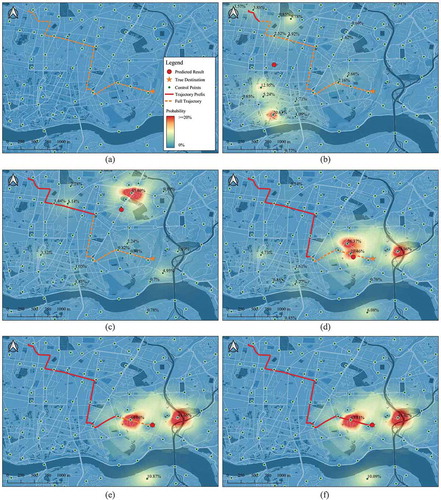
To prove our method can be used in real-time scenarios, we show a step-by-step prediction case as follows: Figure 5 presents an example of destination prediction of one entire trajectory. The prediction results under six different completion scenarios were marked as red dot symbols. We can clearly see that the prediction results moved ahead on their own prefixes. Also, with the increase of prefix completion, the prediction results were getting closer to the real destination of the full trajectory. In this case, the predictions were very close to the real destination when the completions were higher than 60%. From the spatial distribution of probability, we can see that the distribution of probability was more scattered in geographic space when the prefix completion was low, and it became more spatially concentrated when the prefix completion increases. However, even when the completion was 98%, the probability distribution still had multiple aggregation centres. It means the prediction was always determined by a variety of complex factors together rather than a single dominant factor. Therefore, although some regions have very high probabilities, the prediction results will not fall in this region entirely but will be constrained by all control points. It makes the process of destination prediction more reasonable.

Figure 5. An example of destination prediction under six different completion scenarios of a full trajectory. Control points with a probability greater than 0.5% are labelled. As the completion increase, the predicted destination of the prefixes is gradually approaching the real destination. (a) Trajectory completion: 0%. (b) Trajectory completion: 8%. (c) Trajectory completion: 43%. (d) Trajectory completion: 68%. (e) Trajectory completion: 82%. (f) Trajectory completion: 98%.

4.3 Assessments of destination prediction

4.3.1 Assessment metrics

We measure the performance of every model based on the metrics of Mean Error ($ME$), Error Variance ($EV$), and Accuracy over a fixed error range d ($AC{C}_d$). These metrics are designed to reflect the performance and stability of the model from different perspectives. $ME$ is a basic metric of the overall performance of the models.

(12) $ME=\frac{1}{n}\sum _{i=1}^n{e}_i,$(12)

where $e_i$ means the error of sample $i$ measured by Haversine Distance.

$EV$ reflects the error fluctuations of the model for different test samples.

(13) $EV=\frac{1}{n\text{-}1}\sum _{i=1}^n{(e_i\text{-}ME)}^2.$(13)

The prediction accuracy within a given error range reflects the error distribution over different spatial distances, which can be indicated by $AC{C}_d$.

(14) $AC{C}_d=\frac{\#\left\{\tau \right|e_{\tau }\le d,\tau \in T_{test}\}}{\#\left\{\tau \right|\tau \in T_{test}\},}$(14)

where $d$ denotes the error range expressed in kilometres, and $\tau$ is a sample from the test dataset. The hash symbol, #, denotes the number of samples of set $\{\tau \}$ in this equation.

4.3.2 Performance comparison with the state-of-the-art models

We conduct a comprehensive comparison among our method, other existing works, and the baseline method. In this paper, we regard the Cart Decision Tree (DT) as a baseline regressor because it is simple and works in most cases. In addition, the model structure of LSTM with Trajectory Node Points (LSTM-TNP) and DND is basically the same. The main difference is that the LSTM-TNP uses trajectory node points as inputs. Hence, comparing results between the two models can prove that the TNV can improve the predicting performance.

In order to verify the performance of our method, we compare the DND with existing models which are listed in Table 1. To test the TSV’s capability of trajectory representation, we train all these models without any metadata of taxi trips but GPS coordinates only. All the models are trained on the same training dataset and test dataset, as described in experimental setup.

Table 1. Models for performance comparison.

Abbreviation	Source	Year	Data	Description
TCONV-LE	Lv et al.	2018	points to images	A convolutional neural network based model, which converts data into images to keep the spatial relationship between trajectory data. It is currently one of the best performing models on the ECML-PKDD dataset.
DPNLP	Fan et al.	2018	points to embeddings	A deep learning based model combines convolutional neural network and recurrent neural network. It extracts spatial features by obtaining the relationship between locations in traffic network.
LSTM-TNP	-	-	points of trajectory nodes	An LSTM neural network reads trajectory nodes one by one. It uses longitude and latitude as the inputting features for each trajectory node.
MLP	de Brébisson et al.	2015	points	A multi-layer perceptron model won the ECML/PKDD challenge. It only uses the latitudes and longitudes of the first and last 5 points in the trajectory.
RNN	de Brébisson et al.	2015	points	A recurrent neural network, reads GPS points one by one and updates a fixed-length internal state with the same transition matrix at each time step.
Bi-RNN	de Brébisson et al.	2015	points	A bidirectional recurrent neural network, which regards a trajectory as a sequence of GPS points. This model uses a sliding window of 5 successive GPS points as a transition state of RNN.

The result shows that our method achieves a mean error of 1.08 km, which is obviously superior to other models. Table 2 illustrates that DND performed much better on both accuracy and stability, according to $ME$ and $EV$. Furthermore, within the given error ranges,1 km, 2 km and 3 km, the accuracy of DND also surpasses those of other methods, especially when $AC{C}_1$ exceeding 64% and $AC{C}_3$ close to 93%. Given the whole study area covers more than 488.04 square kilometres, these figures show that DND is valuable for practical applications. In comparison with the baseline model, we can find out that RNN and Bi-RNN achieve satisfactory results. TCONV-LE and DPNLP perform obviously better because they both use convolutional layers to obtain contextual features. Although DND is a structural analogue of RNN-based model, it achieves the best results in all metrics among all these models. Therefore, we speculate that TNV and TSV can efficiently capture neighbouring and distant dependencies that greatly help DND to promote its prediction accuracy and stability. Finally, LSTM-TNP’s results are clearly worse than DND’s, which proves that TNV is helpful in performance improvement.

Table 2. Performance comparison, both the units of $ME$ and $EV$ are kilometres.

Metrics	DND	TCONV-LE	DPNLP	LSTM-TNP	MLP	RNN	Bi-RNN	DT
$ME$	1.08	1.25	1.20	1.38	1.38	1.54	1.48	1.99
$EV$	1.77	1.87	1.83	2.09	2.29	2.31	2.46	4.25
$AC{C}_1$	64.12%	58.07%	60.02%	52.94%	55.02%	47.35%	52.07%	40.07%
$AC{C}_2$	85.31%	84.74%	83.58%	79.97%	79.05%	75.17%	76.88%	64.51%
$AC{C}_3$	93.43%	91.86%	92.27%	90.73%	89.53%	87.28%	88.13%	78.39%

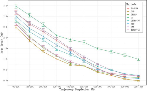
In Figure 6, we can find the prediction error distribution according to different sample trajectory completions. We compare the results of the seven methods above in order to analyse the effect of trajectory completion on prediction errors. We conclude that, for each method, the higher the trajectory completion is, the lower the prediction error is. When the given parts exceed 60%, most models performed closely because of rich premise. However, DND, TCONV-LE and DPNLP are obviously better than other models before this interval. It illustrates that these three models, especially the DND, can predict better results when partial trajectories are in relatively lower completion. We can find that the DND model has an advantage over all completions. From the error bar, we can find that the results of DND are gradually more stable when the trajectory completion rate increases. And the error range of DND is almost within 450 m of the real destination for trajectory completions from 80% to 100%. Moreover, the distance between the DND line and the LSTM-TNP line does not change notably along the trajectory completion axis. It means the TNV works well in all trajectory completions.

Figure 6. Error bar of final destination prediction according to trajectory completion.

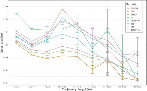
In Figure 7, we display the error distribution according to real trajectory length. According to mean errors, DND performs best among all these methods, especially in long trajectories. As the trajectory length increases, the mean error becomes lower while the prediction stability becomes worse because long trajectory samples are relatively less in real situations and their characteristics vary intensively. It leads to insufficient training for all the methods when trajectories are very long. Remarkably, DND is relatively more stable than other methods when the trajectory length exceeds 24.5 km. Beyond this length, DND’s prediction results were almost within 150 m of the real locations. It confirms our claim that the DND model can well preserve distant dependencies. In addition, the performance difference between LSTM-TNP and DND is more significant in short trajectories. Hence, we speculate that the neighbouring dependencies are more important in shorter trajectories, and the TNV has achieved good results in capturing neighbouring dependencies.

Figure 7. Error bar of final destination prediction according to trajectory length.

4.4 Assessments of TNV and TSV

Through the following two experiments, we studied the trajectory representation capabilities of TNV and TSV, respectively. The first one is to confirm the close relationship between vector similarity and spatial proximity, based on TNVs. In the second experiment, by clustering TSVs, we found a significant correlation between the distribution characteristics of trajectory in geographic space and the clustering category of trajectory in vector space.

4.4.1 Relationship between TNV similarity and geospatial proximity

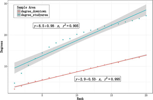
The assessment was conducted on two trajectory node datasets. The first dataset was randomly selected from the original dataset in the study area, which covered 8,480 non-repeating road junctions. The other one filtered 3,631 non-repeating nodes located in the downtown of Porto from the first sample. In this case, we defined the similarity of trajectory nodes as the cosine distance between two TNVs. For each node in the dataset, we choose 20 most similar nodes from all nodes in the study area. Then, we rank these similar nodes according to their similarity from high to low and calculate Euclidean distance and degrees among all the node pairs. Here, degrees denote the shortest path between two nodes on the topological structure of the road network. As shown in Figures 8 and 9, both the mean Euclidean distance and mean degrees show a clear linear relationship with TNV similarity rank. The above two indicators are relatively close when the rank is small. In particular, when the rank equals 1, the mean Euclidean distances are 733 m (study area), 303 m (downtown), and the mean degrees are 4.65 (study area), 2.75 (downtown), revealing that the greater the cosine similarity between two TNVs is, the closer the trajectory nodes are in a geographic space. It also demonstrates that TNVs can represent neighbouring dependencies. However, the linear relationship is better in the downtown area, according to its narrower 95% confidence bandwidth. We argue that suburban TNVs are relatively undertrained due to the sparseness of trajectory sample there, which is consistent with the spatial distribution of training data.

Figure 8. Scatter plot of mean Euclidean distance vs TNV similarity rank.

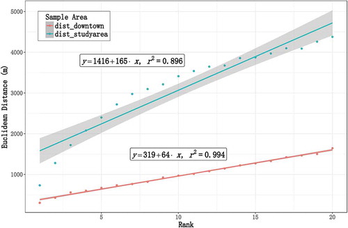
Figure 9. Scatter plot of mean degrees vs TNV similarity rank.

4.4.2 Spatial distribution of TSV clustering

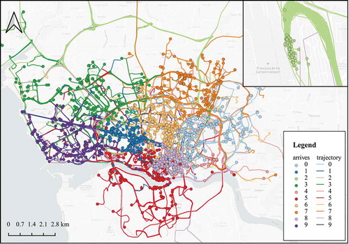
To achieve a better understanding of TSV’s ability to represent distant dependencies, we examined the geographic distribution of TSV clustering results by K-means. In this experiment, the testing dataset, described in 4.1, was clustered into 10 categories according to TSV. In Figure 10. we find that different categories of trajectories have distinct spatial distributions. Moreover, their destination distribution divides the geographic space into 10 highly homogeneous regions. It means TSV can keep relations between the prefix trajectories and their final destinations. Especially, as illustrated on the top right of Figure 10, the destinations of category 2 are concentrated near the airport. From another point of view, TSV has learned the macro characteristics of trajectories that represent distant dependencies, because the destination of the prefix is mainly reflected by its macro characteristics.

Figure 10. Geographic distribution of TSV clusters in Porto.

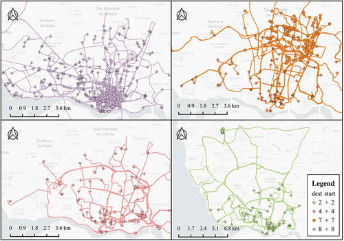
In Figure 11, we can see that despite trajectories of the same category differed on their position and geometry, and their destinations are located relatively concentrated. It reveals that TSV can learn more abstract relations between prefixes and destinations other than just finding morphologically similar trajectories. In addition, the start points cover a very wide range in the geographic region. We concluded that TSV can represent distant dependencies in a relatively wide geographic space. More interestingly, the clustering results demonstrate that trajectories arriving at different destinations have different preferences of road choice. Also, the results clearly reflect these distinct road selection patterns.

Figure 11. Start point distribution, destination distribution and road selection patterns of different TSV clustering results.

5. Conclusion and future work

In this paper, we proposed a novel trajectory modelling method that transforms original trajectories into fixed-length vectors from variable-length sequences with neighbouring and distant dependencies embedded. This method can learn road network topological structure from historical trajectory data and is machine learning friendly. We conducted comprehensive experiments on real taxi trajectory dataset. The results demonstrated that: (1) TNV can capture the neighbouring dependencies while TSV can represent the distant dependencies; (2) TNV can notably improve the destination prediction performance; (3) Our destination prediction model based on TSV achieved a mean error of 1.10 km, which performed much better than other referred methods; (4) This new method takes a significant advantage in destination predicting for long trajectories.

Based on the findings of this paper, we will focus on three research directions in the future. First, our method is not very effective to achieve good results for non-vehicle trajectories. We intend to extend this method further to represent and predict walking trajectories. Second, we can make further attempts in more applications by extending this method, i.e. in the transportation field, trajectory models are applied to demand estimation, designing public transit and even emergency response (Markovic et al. 2018). In the security field, vehicle trajectory data have been used to investigate the road network conditions and reveal important facts about human behaviours after an earthquake (Hara and Kuwahara 2015). Third, the complexity of our model is quite high. How to optimize the model structure and speed up the calculation remains a challenge.

Disclosure statement

No potential conflict of interest was reported by the authors.

Additional information

Funding

This work was supported by the National Key Research and Development Program of China [2017YFB0503500]; the National Natural Science Foundation of China [41571382,41601499]; Jiangsu Province Surveying and Mapping Geographic Information Research Project [JSCHKY201707]

Notes on contributors

Chengyang Qian

Chengyang Qian is a PhD candidate in Key Laboratory of Virtual Geographic Environment (Nanjing Normal University), Ministry of Education, Nanjing, China. He is also a chief specialist in Intelligent City Research Institute, Suzhou Industrial Park Surveying, Mapping and Geoinformation Co., Ltd, Suzhou, China. Email: [email protected]. His research interests include geographical information science, spatio-temporal data mining, and remote sensing.

Ruqiao Jiang

Ruqiao Jiang is an engineer in Intelligent City Research Institute, Suzhou Industrial Park Surveying, Mapping and Geoinformation Co., Ltd, Suzhou, China. Email: [email protected]. His research interests including geographical information science, digital terrain analysis and urban geography.

Yi Long

Yi Long is a professor in Key Laboratory of Virtual Geographic Environment (Nanjing Normal University), Ministry of Education, Nanjing, China. Email: [email protected]. His research interests include cartography, geography and geographical information science.

Qi Zhang

Qi Zhang is an engineer in Intelligent City Research Institute, Suzhou Industrial Park Surveying, Mapping and Geoinformation Co., Ltd, Suzhou, China. Email: [email protected]. Her research interests including geographical information science, urban geography, and urban computing.

Muxian Li

Muxian Li is an engineer in Intelligent City Research Institute, Suzhou Industrial Park Surveying, Mapping and Geoinformation Co., Ltd, Suzhou, China. Email: [email protected]. His research interests including geographical information science, digital terrain analysis, and urban geography.

Ling Zhang

Ling Zhang is a lecturer in Key Laboratory of Virtual Geographic Environment (Nanjing Normal University), Ministry of Education, Nanjing, China. Email: [email protected], [email protected]. His research interests include map generalization, multi-scale representation, and geoinformatics (GIS).

Notes

1. https://www.kaggle.com/c/pkdd-15-predict-taxi-service-trajectory-i.

References

- Bengio, Y., Courville, A., and Vincent, P., 2013. Representation learning: a review and new perspectives. IEEE Transactions on Pattern Analysis and Machine Intelligence, 35 (8), 1798–1828. doi:10.1109/TPAMI.2013.50.
- Besse, P.C., et al., 2018. Destination prediction by trajectory distribution-based model. IEEE Transactions on Intelligent Transportation Systems, 19 (8), 2470–2481. doi:10.1109/TITS.2017.2749413.
- Bogorny, V., Kuijpers, B., and Alvares, L.O., 2009. ST-DMQL: a semantic trajectory data mining query language. International Journal of Geographical Information Science, 23 (10), 1245–1276. doi:10.1080/13658810802231449.
- de Brébisson, A., et al., 2015. Artificial neural networks applied to taxi destination prediction. arXiv Preprint arXiv. 1508.00021.
- Fan, X., et al., 2018. A deep learning approach for next location prediction. In: 2018 IEEE 22nd international conference on Computer Supported Cooperative Work in Design ((CSCWD)), 9-11 May 2018 Nanjing. IEEE, 69–74.
- Firth, J.R., 1957. A synopsis of linguistic theory, 1930–1955. In: Studies in linguistic analysis. Oxford: Blackwell, 1–32.
- Furtado, A.S., et al., 2018. Unveiling movement uncertainty for robust trajectory similarity analysis. International Journal of Geographical Information Science, 32 (1), 140–168. doi:10.1080/13658816.2017.1372763.
- Gao, Q., et al., 2017. Identifying human mobility via trajectory embeddings. In: Proceedings of the 26th international joint conference on artificial intelligence. California, 1689–1695.
- Guo, D., et al., 2018. Detecting spatial community structure in movements. International Journal of Geographical Information Science, 32 (7), 1326–1347. doi:10.1080/13658816.2018.1434889.
- Hara, Y. and Kuwahara, M., 2015. Traffic monitoring immediately after a major natural disaster as revealed by probe data – a case in Ishinomaki after the Great East Japan Earthquake. Transportation Research Part A: Policy and Practice, 75, 1–15.
- Harris, Z.S., 1954. Distributional structure. Word, 10 (2–3), 146–162. doi:10.1080/00437956.1954.11659520.
- Hoch, T., 2015. An ensemble learning approach for the Kaggle taxi travel time prediction challenge. In: Proceedings of the 2015th International Conference on ECML PKDD Discovery Challenge -Volume 1526, 7-11 September 2015 Porto. 52–62.
- Hochreiter, S. and Schmidhuber, J., 1997. Long short-term memory. Neural Computation, 9 (8), 1735–1780. doi:10.1162/neco.1997.9.8.1735.
- Krumm, J. and Horvitz, E., 2006. Predestination: inferring destinations from partial trajectories. In: UbiComp 2006: ubiquitous computing, 17-21 September 2006 Orange. Berlin - Heidelberg: Springer, 243–260.
- Lam, H.T., et al., 2015. (Blue) taxi destination and trip time prediction from partial trajectories. In: Proceedings of the 2015th International Conference on ECML PKDD Discovery Challenge - Volume 1526, 7-11 September 2015 Porto. 63–74.
- Liu, Q., et al., 2016. Predicting the next location: a recurrent model with spatial and temporal contexts. In: Proceedings of the thirtieth AAAI conference on artificial intelligence, 12-17 February 2016 Phoenix. 194–200.
- Lv, J., et al., 2018. T-CONV: a convolutional neural network for multi-scale taxi trajectory prediction. In: 2018 IEEE international conference on big data and smart computing (bigcomp), 15-18 January 2018 Shanghai. 82–89.
- Magdy, N., Sakr, M.A., and Mostafa, T., 2015. Review on trajectory similarity measures. In: 2015 IEEE seventh international conference on Intelligent Computing and Information Systems (ICICIS), 12-14 December 2015 Cairo. 613–619.
- Markovic, N., et al., 2018. Applications of trajectory data from the perspective of a road transportation agency: literature review and maryland case study. IEEE Transactions on Intelligent Transportation Systems, 20(5), 1–12.
- Mazimpaka, J.D. and Timpf, S., 2016. Trajectory data mining: A review of methods and applications. Journal of Spatial Information Science, 13, 61–99.
- Mikolov, T., et al., 2013. Efficient estimation of word representations in vector space. arXiv Preprint arXiv. 1301.3781.
- Newson, P. and Krumm, J., 2009. Hidden Markov map matching through noise and sparseness. In: Proceedings of the 17th ACM SIGSPATIAL international conference on advances in geographic information systems. Seattle, Washington, 336–343.
- Tanaka, K., et al., 2009. A destination prediction method using driving contexts and trajectory for car navigation systems. In: Proceedings of the 2009 ACM symposium on applied computing, 9-12 March 2009 Honolulu. ACM, 190–195.
- Turian, J., Ratinov, L., and Bengio, Y., 2010. Word representations: a simple and general method for semi-supervised learning. In: Proceedings of the 48th annual meeting of the association for computational linguistics. Uppsala, Sweden, 384–394.
- Wang, L., et al., 2017. Moving destination prediction using sparse dataset: a mobility gradient descent approach. ACM transactions on knowledge discovery from data, 11 (3), 37. doi:10.1145/3051128.
- Wu, H., et al., 2017. Modeling trajectories with recurrent neural networks. In: Proceedings of the 26th international joint conference on artificial intelligence IJCAI-17. Melbourne, Australia, 3083–3090.
- Xiao, X., et al., 2010. Finding similar users using category-based location history. In: Proceedings of the 18th SIGSPATIAL international conference on advances in geographic information systems, 2-5 November 2010 San Jose. ACM, 442–445.
- Xie, D., Li, F., and Phillips, J.M., 2017. Distributed trajectory similarity search. In: Proceedings of the 43rd International Conference on Very Large Data Bases, 28 August - 1 September 2017 Munich. ACM, 1478–1489.
- Xue, A.Y., et al., 2013. Destination prediction by sub-trajectory synthesis and privacy protection against such prediction. In: 2013 IEEE 29th international conference on data engineering (ICDE), 8-12 April 2013 Brisbane. IEEE, 254–265.
- Yao, D., et al., 2017. SERM: a recurrent model for next location prediction in semantic trajectories. In: Proceedings of the 2017 ACM on conference on information and knowledge management - CIKM ’17. New York, New York, USA: ACM Press, 2411–2414.
- Yao, D., et al., 2018. Learning deep representation for trajectory clustering. Expert Systems, 35 (2), 1–16. doi:10.1111/exsy.12252.
- Ying, J.J.C., et al., 2011. Semantic trajectory mining for location prediction. In: Proceedings of the 19th ACM SIGSPATIAL international conference on advances in geographic information systems. Chicago, Illinois, 34–43.
- Zhang, L., et al., 2016. Sparse trajectory prediction based on multiple entropy measures. Entropy, 18 (9), 327. doi:10.3390/e18090327.
- Zhou, N., et al., 2016. A general multi-context embedding model for mining human trajectory data. IEEE Transactions on Knowledge and Data Engineering, 28 (8), 1945–1958. doi:10.1109/TKDE.2016.2550436.
- Ziebart, B.D., et al., 2008a. Maximum entropy inverse reinforcement learning. In: Proceedings of the 23rd national conference on Artificial intelligence, 13-17 July 2008 Chicago. AAAI, 1433–1438.
- Ziebart, B.D., et al., 2008b. Navigate like a cabbie: probabilistic reasoning from observed context-aware behavior. In: Proceedings of the 10th international conference on Ubiquitous computing, 21-24 September 2008 Seoul. ACM, 322–331.