Spatio-temporal regression kriging for modelling urban NO₂ concentrations

ABSTRACT

Recently developed urban air quality sensor networks are used to monitor air pollutant concentrations at a fine spatial and temporal resolution. The measurements are however limited to point support. To obtain areal coverage in space and time, interpolation is required. A spatio-temporal regression kriging approach was applied to predict nitrogen dioxide (NO₂) concentrations at unobserved space-time locations in the city of Eindhoven, the Netherlands. Prediction maps were created at 25 m spatial resolution and hourly temporal resolution. In regression kriging, the trend is separately modelled from autocorrelation in the residuals. The trend part of the model, consisting of a set of spatial and temporal covariates, was able to explain 49.2% of the spatio-temporal variability in NO₂ concentrations in Eindhoven in November 2016. Spatio-temporal autocorrelation in the residuals was modelled by fitting a sum-metric spatio-temporal variogram model, adding smoothness to the prediction maps. The accuracy of the predictions was assessed using leave-one-out cross-validation, resulting in a Root Mean Square Error of 9.91 μg m⁻³, a Mean Error of −0.03 μg m⁻³ and a Mean Absolute Error of 7.29 μg m⁻³. The method allows for easy prediction and visualization of air pollutant concentrations and can be extended to a near real-time procedure.

KEYWORDS:

• Spatio-temporal kriging
• variogram
• air quality
• sensor network
• nitrogen dioxide

1. Introduction

Geo-information science supports the computation and visualization of large amounts of spatio-temporal data. In combination with spatio-temporal statistics, prediction maps can be made, for example, to visualize air pollution. Air pollution is worldwide a major cause of morbidity and mortality (Cohen et al. 2017) and national air quality monitoring networks have been set up to monitor whether it exceeds legal limit levels. Due to the high costs of the instruments, their maintenance and validation, the number of measurement locations is typically limited to one or two in each city. Low-cost air quality sensor networks, measuring pollutant concentrations at a fine spatio-temporal resolution at an urban scale level, are gaining interest (Snyder et al. 2013). These networks can be operated for a longer period of time (>1 year) and can be used to model air pollution at a fine spatial and temporal resolution.

Modelling air pollutant concentrations is done with the aim to predict air pollutant concentrations at unmeasured locations. Land use regression (LUR) models, referring to regression models including land use covariates from a geo-information system (Hoek et al. 2008), are used for modelling fine-scale variation in the air quality at an urban scale level. In most LUR studies, the models are used to obtain seasonal or annual average predictions (Lee et al. 2017, Kashima et al. 2018, Weissert et al. 2018). These are suited for applications where mostly spatial variability is of importance, such as policy decisions regarding polluted areas of a city or assessing long-term health effects of air pollution. All temporal variation will be neglected when an LUR model is used to predict annual mean concentrations, leading to a loss of precision and power (Klompmaker et al. 2015). The spatial covariates in an LUR model will also not be able to account for all spatial variability, nor for spatial autocorrelation in the residuals.

When a regression model is combined with spatial kriging, the spatial autocorrelation structure can be accounted for. Spatial kriging is then used to interpolate the concentration values between different measurement locations (Beelen et al. 2009, Van de Kassteele et al. 2009). To account for temporal variability and temporal autocorrelation, the regression model can be extended to include temporal covariates, and the residuals of the model can be interpolated using spatio-temporal kriging (Kilibarda et al. 2014, Hu et al. 2015). A spatio-temporal variogram function is then used to describe the spatio-temporal autocorrelation structure (Gräler et al. 2016).

The main objective of this study is to model spatio-temporal variability in urban air pollutant concentrations using a spatio-temporal regression kriging model. We applied the method on a low-cost urban air quality sensor network in the city of Eindhoven, the Netherlands (Close 2016), focusing on NO₂.

2. Methods

2.1. Model formulation

We consider a sensor network with $N_s$ number of sensor locations $s_i$, $i=\left\{1,\dots ,N_s\right\}$. The sensor measurements are taken at point support in space, represented by a two-dimensional set of spatial coordinates for each sensor location. At the sensor location $s_i$, the air pollutant concentration $NO2\left(s_i,t_j\right)$ is stored for each of the $N_t$ number of time stamps $t_j$, $j=\left\{1,\dots ,N_t\right\}$. Each time stamp denotes the end of an hourly averaging period.

We modelled the air pollutant concentration $NO2\left(s_i,t_j\right)$ with mean $\mu \left(s_i,t_j\right)$ and residual $\eta \left(s_i,t_j\right)$:

(1) $NO2\left(s_i,t_j\right)=\mu \left(s_i,t_j\right)+\eta \left(s_i,t_j\right)$(1)

The mean $\mu \left(s_i,t_j\right)$ incorporates the trend component of the model, consisting of a linear combination of covariate values $x_c$ from a set of spatial and temporal covariates $C$. The trend part of the model is estimated as:

(2) $\hat{\mu }\left(s_i,t_j\right)={\hat{\beta }}_0+{\sum }_C{\hat{\beta }}_c{x}_c\left(s_i,t_j\right)$(2)

Here ${\hat{\beta }}_0$ is the estimated intercept and ${\hat{\beta }}_c$ are the estimated regression coefficients for covariates $c\in C$, based on ordinary least squares.

After estimating the parameters and predicting $\hat{\mu }\left(s_i,t_j\right)$ at each observed space-time location $\left(s_i,t_j\right)$, we model the spatio-temporal autocorrelation in the residuals. We take the residuals as the differences between the observations and the estimated trend, and in this approach we ignore any uncertainties in the estimated trend. Their inclusion could be part of future research. The distribution of the residuals is visually checked for normality. To explore the spatio-temporal dependency in the residuals, we use the spatio-temporal variogram (Cressie and Wikle 2011, Sherman 2011). The spatio-temporal variogram represents the semivariance between any pair of residuals which are separated by spatial lag $h$ and/or temporal lag $u$:

(3) $\gamma \left(h,u\right)=\frac{1}{2}\mathbb{E}{\left(\eta \left(s_i,t_j\right)-\eta \left(s_i+h,t_j+u\right)\right)}^2$(3)

Here, $\mathbb{E}$ denotes the expected value. A spatio-temporal sample variogram is formed by averaging the semivariance in regularly spaced spatio-temporal bins, similar to standard spatial variograms. A space-time variogram model is fitted to the spatio-temporal sample variogram. Based on the smallest mean square error (MSE) between the sample variogram and fitted variogram we fitted a sum-metric space-time variogram model. The sum-metric model combines a spatial, temporal and metric model accounting for space-time anisotropy (Gräler et al. 2016):

(4) $\gamma \left(h,u\right)=\gamma \left(h\right)+\gamma \left(u\right)+\gamma \left(\sqrt{h^2+{\left(\kappa \times u\right)}^2}\right)$(4)

where $\gamma \left(h,u\right)$ is the space-time variogram, $\gamma \left(h\right)$ is the spatial variogram, $\gamma \left(u\right)$ is the temporal variogram, $\gamma \left(\sqrt{h^2+{\left(\kappa \times u\right)}^2}\right)$ is the joint variogram, and $\kappa$ is a spatio-temporal anisotropy scaling parameter. This requires estimation of $\kappa$, as well as a set of spatial variogram model parameters ${\theta }_s=\left\{{\tau }_s^2,{\sigma }_s^2,{\varphi }_s\right\}$, a set of temporal variogram model parameters ${\theta }_t=\left\{{\tau }_t^2,{\sigma }_t^2,{\varphi }_t\right\}$ and a set of joint variogram model parameters ${\theta }_{joint}=\left\{{\tau }_{joint}^2,{\sigma }_{joint}^2,{\varphi }_{joint}\right\}$. Each set of parameters contains, respectively, the nugget, partial sill and range of – in our case – a spherical variogram model (Zimmerman and Stein 2010). The nugget consists of two components: microscale variance and variance induced by inaccuracies in the measurement device (Cressie and Wikle 2011). The partial sill and range affect the shape of the variogram model. Depending on the spatio-temporal autocorrelation of the pollutant, different pollutants have different variogram models. Variogram model parameter estimation is done through optimization using the bound constrained BFGS method (Byrd et al. 1995). We assume isotropy and stationarity in space and time, which allows for the same variogram to be used in all directions and at all spatio-temporal locations.

2.2. Spatio-temporal predictions

We combine the estimated parameters of the regression model and the estimated semivariance parameters to predict the NO₂ concentration $\widehat{NO2}\left(s_0,t_0\right)$ at any unobserved spatio-temporal location $\left(s_0,t_0\right)$ located on a spatio-temporal prediction grid:

(5) $\widehat{NO2}\left(s_0,t_0\right)=\hat{\mu }\left(s_0,t_0\right)+\hat{\eta }\left(s_0,t_0\right)$(5)

where the predicted trend component $\hat{\mu }\left(s_0,t_0\right)={\hat{\beta }}_0+\sum _c{\hat{\beta }}_c{x}_c\left(s_0,t_0\right)$ is based on the covariate values $x_c\left(s_0,t_0\right)$ at spatio-temporal prediction location $\left(s_0,t_0\right)$. Kriging gives us the Best Linear Unbiased Predictor (BLUP) of the residual component, $\hat{\eta }\left(s_0,t_0\right)={\lambda }_0\bar{\eta }$, where $\bar{\eta }$ is a vector of observed space-time residuals and ${\lambda }_0$ is a vector of kriging weights (Diggle and Ribeiro 2007). The kriging weights express the strength of the association between observation locations and the prediction location, estimated as ${\lambda }_0={\gamma }_0^T{\mathrm{\Gamma }}^{-1}$. Here, ${\gamma }_0$ is a vector containing the semivariances between the observation locations and the prediction location $\left(s_0,t_0\right)$, and $\mathrm{\Gamma }$ is a matrix containing the semivariances between all possible combinations of space-time observations. We apply simple kriging, as we assume the residuals to have a known mean of zero.

The prediction maps on the full space-time grid were accompanied with kriging variance maps to evaluate the uncertainty of the kriging predictions. The kriging variance ${\sigma }_0^2$ at a prediction location $\left(s_0,t_0\right)$ is defined as (Webster and Oliver 2001):

(6) ${\sigma }_0^2={\gamma }_0^T{\mathrm{\Gamma }}^{-1}{\gamma }_0$(6)

Variogram parameter estimation and spatio-temporal kriging were done in R using the ‘gstat’ package (Gräler et al. 2016). The used code is available from the authors upon request. Spatio-temporal kriging is computationally demanding, as it requires computation of the inverse of the spatio-temporal semivariance matrix at every location on the spatio-temporal prediction grid. To improve efficiency and to reduce computation time, we limit the temporal observation locations used for predictions, i.e. perform local kriging on the temporal part. While using all spatial locations, we limit the number of temporal neighbors to those within a temporal distance of $\mathrm{m}\mathrm{a}\mathrm{x}\left({\varphi }_t,{\varphi }_{joint}/\kappa \right)$, rounded up to the next whole number. This should not meaningfully influence the predictions, as the kriging weights approach zero when $u>\mathrm{m}\mathrm{a}\mathrm{x}\left({\varphi }_t,{\varphi }_{joint}/\kappa \right)$.

2.3. Validation

To evaluate the accuracy of the kriging predictions, we performed leave-one-out cross-validation (LOOCV) at all observed space-time locations $\left(s_i,t_j\right)$. For one space-time location $\left(s_i,t_j\right)$ at a time, the value $\eta \left(s_i,t_j\right)$ is removed from the dataset. The remainder of the dataset, temporally limited to $t_j\pm \mathrm{m}\mathrm{a}\mathrm{x}\left({\varphi }_t,{\varphi }_{joint}/\kappa \right)$, is used to predict $\hat{\eta }\left(s_i,t_j\right)$. This process is repeated for each observed space-time location $\left(s_i,t_j\right)$. The Root Mean Square Error (RMSE) is then used to assess the accuracy of the kriging predictions:

(7) $RMSE=\sqrt{\frac{1}{N_s{N}_t}{\sum }_{i=1,j=1}^{N_s,N_t}{\left(\widehat{NO2}\left(s_i,t_j\right)-NO2\left(s_i,t_j\right)\right)}^2}$(7)

as well as the Mean Error (ME):

(8) $ME=\frac{1}{N_s{N}_t}{\sum }_{i=1,j=1}^{N_s,N_t}\left(\widehat{NO2}\left(s_i,t_j\right)-NO2\left(s_i,t_j\right)\right)$(8)

and Mean Absolute Error (MAE):

(9) $MAE=\frac{1}{N_s{N}_t}{\sum }_{i=1,j=1}^{N_s,N_t}\left(\left|\widehat{NO2}\left(s_i,t_j\right)-NO2\left(s_i,t_j\right)\right|\right)$(9)

3. Application

Our application concerns an air quality sensor network in the city of Eindhoven. Eindhoven is a medium-sized city in the Netherlands with around 230,000 inhabitants and a total area of 88.84 km². The spatio-temporal variability in air pollutant concentrations is measured using the AiREAS civil initiative air quality measurement network (Close 2016) which has continuously been operating since November 2013. The airboxes in the network measure particulate matter (PM), ozone (O₃) and NO₂ at 2.5–3 m height. We focused on NO₂ air pollution which has a large spatiotemporal variation and a large impact on human health. The NO₂ sensors were calibrated in the field at the end of 2015. More information about the data quality of the airbox NO₂ data can be found elsewhere (Van Zoest et al. 2019).

Figure 1. Locations of the airboxes in Eindhoven which were used for this study. The black line represents the municipal boundary. The coloured lines represent major roads.

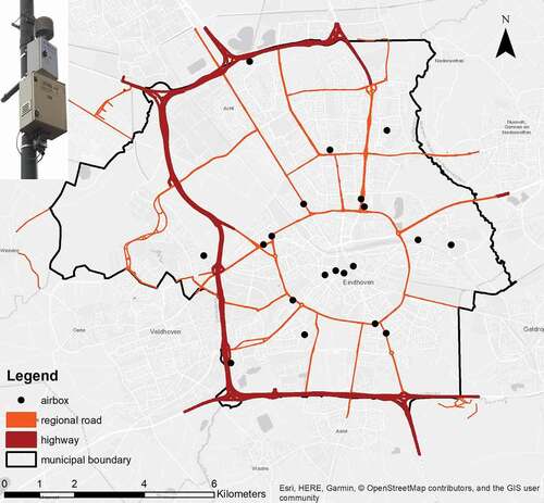
We estimated the model parameters for 1 month of data at a time, to account for sensor drift and seasonal variability in the regression coefficients and semivariance parameters. As an illustration of the method, we used in this study hourly data from November 2016, when NO₂ data were available for 20 airbox locations (Figure 1). The airboxes measure NO₂ every 10 min, and the data were averaged to hourly concentration values to reduce noise and to match the data with the temporal support of the meteorological covariates. Data cleaning and outlier removal were performed as described in Van Zoest et al. (2018) and missing values (9.8%) in each airbox were imputed using regression on the NO₂ values of the remaining airboxes, following Harrell (2018). The observed hourly average NO₂ concentrations varied between 0 and 96 µg m⁻³ in November 2016.

The main source of NO₂ is traffic inside the city and it may be trapped in street canyons between high buildings, especially in the areas with a high population density. In the trend part of the model, three spatial covariates and five temporal covariates were included, which significantly affected the NO₂ concentrations at significance level $\alpha =0.05$ as shown in the 'Results' section (4.1). This set of covariates$C=\left\{pop,road,east,RH,WS,WD,hour,w\right\}$ contains population density ($pop$), road type ($road$), easting coordinates ($east$), relative humidity ($RH$), wind speed ($WS$), wind direction ($WD$), hour of the day ($hour$) and weekday/weekend ($w$), respectively. The final prediction model then becomes:

(10) $\begin{array}{rl}& \widehat{NO2}\left(s_0,t_0\right)={\hat{\beta }}_0+{\hat{\beta }}_{pop}{x}_{s_0}^{pop}+{\hat{\beta }}_{road}{x}_{s_0}^{road}+{\hat{\beta }}_{east}{x}_{s_0}^{east}+{\hat{\beta }}_{RH}{x}_{t_0}^{RH}+{\hat{\beta }}_{WS}{x}_{t_0}^{WS}\\ & +{\hat{\beta }}_{WD}{x}_{t_0}^{WD}+{\hat{\beta }}_{hour}{x}_{t_0}^{hour}+{\hat{\beta }}_w{x}_{t_0}^w+{\gamma }_0^T{\mathrm{\Gamma }}^{-1}\bar{\eta }\end{array}$(10)

Population density was obtained as the number of inhabitants km⁻², from Statistics Netherlands (CBS 2018) at neighborhood level. The lattice data were converted to a raster with a grid cell size of 25 m, similar to the spatial resolution of the prediction grid. Road type data were obtained from the topographic base dataset TOP10NL (Kadaster 2018). We reclassified the road types to distinguish between small roads (width 2–7 m) and main roads (width >7 m). In rasterizing the vector data to fit the prediction grid, any raster cell containing a piece of road was classified as a road cell. The distinction between small roads and main roads was based upon the maximum combined area of each road type overlapping with the raster cell. Easting coordinates were included as the coordinates of the prediction grid. Relative humidity, wind speed and wind direction are centrally monitored at the Royal Netherlands Meteorological Institute weather station in Eindhoven (KNMI 2016) and are therefore considered as temporal covariates only. We distinguish between weekdays and weekends, since the traffic patterns are highly different during weekdays as compared to weekends, thus causing different air pollutant concentrations. Similarly, we include hour of the day in the model to account for diurnal variability in traffic intensity and weather. The prediction grid has a temporal resolution of 1 h.

4. Results and discussion

4.1. Model parameter estimation

The regression model, representing the spatio-temporal trend part of the model, explained 49.2% of the variability in NO₂ concentrations in Eindhoven in November 2016. The estimated coefficients and their p-values are shown in Table 1. Population density was positively related to NO₂ concentrations, as areas with higher population density tend to have a higher traffic intensity and more high-rise buildings. Areas between high-rise buildings form street canyons in which the pollutants are easily trapped. Road type is related to the amount of traffic and therefore an important predictor of air pollution. Especially the presence of main roads had a large influence on the NO₂ concentrations, due to the higher traffic intensity. Easting is a case study area-specific covariate, which is likely related to the prevailing west/south-west wind direction and accumulation of air pollution in the east. Relative humidity and wind speed were negatively related to NO₂ concentrations. A higher wind speed dilutes the pollutant concentrations in the air and therefore naturally leads to lower NO₂ concentrations. Wind direction was related to the temporal variability in NO₂ concentrations, with winds from the South, South-East, East, North-East and North leading to lower NO₂ concentrations than winds from the South-West, West and North-West. The β coefficients of the latter three wind directions were not significantly different from zero, the baseline β coefficient for calm or variable winds.

Table 1. $\hat{\beta }$ and p-values for the trend part of the regression model. The baseline for road type is ‘no road’. The baseline wind direction is ‘calm/variable’, the baseline weekday/weekends is ‘weekday’, and the baseline for hour is ‘0ʹ (23:00–0:00).

Covariate	Covariate unit	$\hat{\beta }$	p-value
Intercept	N/A	−113.38	<0.001
Population density	Inhabitants km^−2 (x1000)	1.47	<0.001
Road type: Small roads	Factor	0.59	0.02
Road type: Main roads	Factor	16.16	<0.001
Easting	km	0.82	<0.001
Relative humidity	%	−0.07	<0.001
Wind speed	m s^−1	−1.03	<0.001
Wind dir.: North	Factor	−2.11	<0.001
Wind dir.: North-East	Factor	−2.00	<0.001
Wind dir.: East	Factor	−4.23	<0.001
Wind dir.: South-East	Factor	−2.67	<0.001
Wind dir.: South	Factor	−1.76	<0.001
Wind dir.: South-West	Factor	0.19	0.71
Wind dir.: West	Factor	−0.92	0.10
Wind dir.: North-West	Factor	−1.28	0.07
Weekday: Weekend	Factor	−3.79	<0.001
Hour: 1	Factor	−1.61	0.004
Hour: 2	Factor	−2.25	<0.001
Hour: 3	Factor	−2.97	<0.001
Hour: 4	Factor	−3.20	<0.001
Hour: 5	Factor	−2.77	<0.001
Hour: 6	Factor	−0.50	0.37
Hour: 7	Factor	2.59	<0.001
Hour: 8	Factor	3.91	<0.001
Hour: 9	Factor	3.29	<0.001
Hour: 10	Factor	2.59	<0.001
Hour: 11	Factor	2.04	<0.001
Hour: 12	Factor	2.14	<0.001
Hour: 13	Factor	2.78	<0.001
Hour: 14	Factor	4.32	<0.001
Hour: 15	Factor	6.03	<0.001
Hour: 16	Factor	8.05	<0.001
Hour: 17	Factor	9.70	<0.001
Hour: 18	Factor	8.99	<0.001
Hour: 19	Factor	6.78	<0.001
Hour: 20	Factor	5.46	<0.001
Hour: 21	Factor	4.68	<0.001
Hour: 22	Factor	4.36	<0.001
Hour: 23	Factor	2.70	<0.001

Relative humidity, wind speed and wind direction cannot be controlled to reduce air pollution in the city. However, policymakers can consider these in spatial planning. Based on prevailing winds from the west/south-west and their impact on the transportation of air pollutants, spatial planners would be advised to locate main sources of air pollution, such as highways and the airport, on the east side of the city. We also observe a strong relationship between NO₂ concentrations and population density. The exposure to air pollutants would be more equally divided amongst inhabitants when spatial planners would step away from the traditional city plan, in which high-rise buildings are clustered in the center and low-rise buildings are clustered in the suburbs. Making main roads smaller might decrease local air pollution, but will likely create congestion and increase air pollution elsewhere.

The residuals follow an approximately normal distribution. The left panel in Figure 2 shows the spatio-temporal sample variogram of the residuals of the fitted regression model, using a temporal bin size of 1 h and a spatial bin size of 500 m. The sample variogram shows some periodicity along the spatial axis, likely due to the limited number of spatial locations on which the variogram is based. The fitted sum-metric variogram model is shown in the right panel of Figure 2. Its MSE of 288 was lowest compared to metric and separable variogram models, as also found in the example shown in Gräler et al. (2016). Visually, the fitted variogram model well represents the overall shape of the sample variogram both in terms of spatial, temporal and joint spatio-temporal dependencies. The estimated parameters of the sum-metric variogram model are shown in Table 2. We observe that the spatial parameters indicate a pure nugget variogram. The spatial dependencies are therefore only considered in the joint variogram model. The temporal dependencies are considered both in the temporal variogram model and in the joint variogram model.

Figure 2. Spatio-temporal sample variogram (left) and sum-metric fitted variogram model (right).

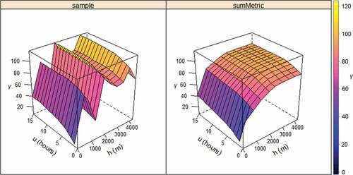
Table 2. Spatio-temporal variogram parameter estimates for the fitted sum-metric variogram.

Parameter	Estimate
${\tau }_s^2$	35.2 (µg m^−3)^2
${\sigma }_s^2$	0.00 (µg m^−3)^2
${\varphi }_s$	2692 m
${\tau }_t^2$	0.00 (µg m^−3)^2
${\sigma }_t^2$	10.8 (µg m^−3)^2
${\varphi }_t$	6.1 hrs
${\tau }_{joint}^2$	10.6 (µg m^−3)^2
${\sigma }_{joint}^2$	40.3 (µg m^−3)^2
${\varphi }_{joint}$	2670 m
$\kappa$	61.1 m hr^−1

4.2. Prediction maps

Figure 3 shows the prediction maps of four time stamps on Monday the 7^th of November 2016. The maps represent the spatial variability as well as the diurnal variability in NO₂ concentrations. The dark blue colors between 2 and 3 a.m. suggest that the concentrations are low. This can be expected during night hours when traffic intensity is low as well. Main roads have a substantially higher NO₂ concentration than small roads within the neighborhoods. The neighborhoods can be clearly distinguished due to the effect of population density. Some smoothing is visible thanks to kriging of the residuals. During rush hours, e.g. between 7 and 8 a.m. and between 5 and 6 p.m., the concentrations are higher than during the night, both at the main roads and at background locations. Especially the air close to the roads south of the center is most polluted with concentrations >40 µg m⁻³. At this location, we find one of the main roads connecting the highway to the city center. At noon, background levels slightly drop, but still, a hotspot exists around the southern main entrance road (red ellipse).

Figure 3. Prediction maps of NO₂ concentrations at four time stamps on Monday the 7th of November, 2016 (UTC time; local time is 1 hour later). The covariate ‘population density’ was included as lattice data, creating clearly distinguished features for the neighborhoods. The red ellipse indicates a hotspot, with locally elevated NO₂ concentrations around the southern main city entrance road.

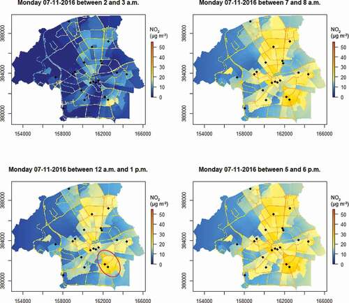
Figure 4. Prediction maps of NO₂ concentrations at four Sundays in November 2016, between 5 and 6 p.m. (UTC time; local time is 1 hour later). Note that different concentration limits were used as compared to Figure 3, to visualize the high concentrations on the 27th of November.

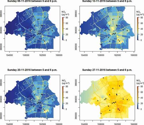
The prediction maps also allow for visual inspection of extreme values. Spatial extremes could be identified as local hotspots on the map. Temporal extremes can be identified by comparing predictions at different time stamps. Figure 4, for example, shows the prediction maps of four different Sundays in November 2016 between 5 and 6 p.m. Clearly, the NO₂ concentrations on the 27^th of November were extremely high throughout the city. The high concentrations on the 27^th of November could not be explained by the meteorological covariates in the trend part of the model, nor by other extreme weather conditions, public events or traffic intensity. However, it should be noted that air pollution levels are based on a very complex combination of sources and sinks, which can be anthropogenic, natural or chemical (Brook et al. 2010, Fenger 2009). Since all airboxes measured high values on the 27^th of November, the extreme values are likely due to a real air pollution event rather than measurement error (Van Zoest et al. 2018).

Prior to the analysis, covariates were selected to be included in the trend part of the model. Some covariates were not included due to a lack of significant association with NO₂ concentrations ($\alpha =0.05$) or lack of improvement in the amount of explained variability. Distance to the nearest road had no significant impact on NO₂ concentrations, because all airboxes were attached to light poles near a road and the variability in distance was only minor. As an alternative, distance to the nearest main road was explored as a covariate. For most airboxes at background air pollution locations, however, these distances were too large to find significant effects. When systematically sampling at different distances from the road smaller than ${\varphi }_s$, it is more likely to find significant effects for this covariate. Instead, we included road type as a factor covariate, distinguishing between no road, small roads and main roads. The difference between the predictions for ‘no road’ and ‘small road’ is small, as can be seen in Table 1 and in the prediction maps. This is no surprise due to the low traffic intensity in smaller streets, practically diluting to background concentrations. We expected distance to the highway to be negatively related to NO₂ but found opposing results, likely because of an inverse relationship between distance to highway and population density. The final model included three spatial covariates and five temporal covariates, a number small enough to avoid overfitting.

4.3. Model performance

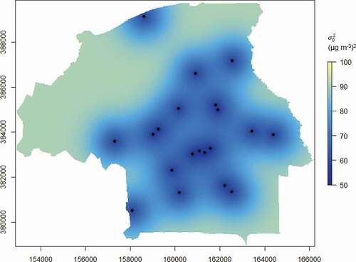
The RMSE obtained using LOOCV was 9.91 μg m⁻³, the ME was −0.03 μg m⁻³ and the MAE was 7.29 μg m⁻³. Due to the use of lattice data for the covariate ‘population density’, the boundaries between neighborhoods are clearly visible on the prediction map. Although this may partly be caused by differences in building patterns, some smoothness is expected. The covariate ‘Easting’ should be interpreted as one specific to the study area, and ${\hat{\beta }}_{east}$ should therefore not be used outside the study area. A combination of this covariate with a low population density on the west side of the study area creates low NO₂ predictions in the western part of the city. No airboxes are located in this area; therefore, the kriging variances are higher here (Figure 5). Due to the airport and highways located in this area, true concentrations could be higher as well.

Figure 5. Kriging variance map (Monday 07-11-2016 between 7 and 8 a.m.).

For the spatial variogram, we found a pure nugget effect. Optimization of the sampling scheme, e.g. by using shorter distances between some of the sensors, may further improve the estimation of the spatial variogram parameters. The sampling scheme in Eindhoven is mostly based on variability in air pollutant concentrations and on the locations of people at risk. Sampling near sources of air pollutants, e.g. the airport, and sampling at different distances from the road may lead to additional covariates of interest and improved model predictions. Further research is needed on sampling scheme optimization, for which the rise of low-cost sensor networks provides valuable opportunities.

5. Conclusions

In this paper, we predicted urban NO₂ concentrations in space and time using a spatio-temporal regression kriging approach. We applied the model on a low-cost urban air quality sensor network in the city of Eindhoven, the Netherlands. A set of spatial covariates, including road type, population density and easting coordinate, and a set of temporal covariates accounting for meteorological variability and periodicity, were included in the trend part of the model. Kriging of the residuals led to more smoothness in the prediction maps compared to a trend model only. Due to the strong temporal variability in the data, spatio-temporal kriging was more useful than spatial kriging. It also allowed for more accurate variogram estimation using all 14400 space-time locations rather than the limited 20 spatial locations. Using the sum-metric variogram model, the spatial and temporal dependencies were not only modelled independently, but also their joint dependencies. In our case of a pure nugget spatial variogram, these joint dependencies were stronger than the purely spatial dependencies.

The method was useful for spatio-temporal prediction of NO₂ in an urban area, where the resulting maps can assist policymakers in infrastructural decision-making and epidemiologists in health risk mapping. They can also improve the development of healthy cyclist route planning (Sharker and Karimi 2014) and they can be of use in outlier detection to distinguish between errors and events (Van Zoest et al. 2018). After the selection of relevant site-specific covariates, the method can be applied in other urban areas where fine resolution urban air quality sensor networks are emerging. While traffic-related covariates are of importance in Eindhoven, other covariates such as distance to factories may be of relevance in highly industrial cities. As the emissions of factories are, like traffic, also dependent on hour of the day and weekday/weekends, including these covariates will likely also be of added value in industrial cities. Interactions between covariates can also be included in the trend part of the model, when enough spatial and temporal locations are available to avoid overfitting.

The estimates of the β coefficients and spatio-temporal variogram parameters should be regularly updated, e.g. every month, to account for drift and seasonal variability in the estimates (Van Zoest et al. 2019). Prediction could be extended to a near real-time procedure in a straightforward way, for example, by creating prediction maps of the air pollutant concentrations each hour. In this way, air pollutant concentrations can be efficiently visualized, allowing for communication with citizens and creating awareness about the quality of the air they breathe.

Disclosure statement

No potential conflict of interest was reported by the authors.

Data and codes availability statement

The data and codes that support the findings of this study are available in DANS with the identifier 10.17026/dans-xmp-fw6h.

Additional information

Funding

This work was supported by the Dutch Research Council (NWO).

Notes on contributors

Vera van Zoest

Vera van Zoest is a PhD candidate at the Faculty of Geo-Information Science and Earth Observation (ITC) at the University of Twente. Her research interests are in spatial data quality analysis, spatio-temporal modelling and geo-health.

Frank B. Osei

Dr. Frank B. Osei is an assistant professor in spatial statistics at ITC, University of Twente. His main research interest surrounds developing and applying spatial statistical methods for environmental and disease data.

Gerard Hoek

Dr. Gerard Hoek is an associate professor at the Institute for Risk Assessment Sciences (IRAS) at Utrecht University. His research focuses on methods for improved exposure assessment to environmental stressors, with a focus on outdoor air pollution.

Alfred Stein

Prof. Alfred Stein is professor in spatial statistics and image analysis at ITC, University of Twente. His main research fields concern spatial and spatio-temporal statistics, including issues of data quality and its revision in geographic information systems.

References

- Beelen, R., et al., 2009. Mapping of background air pollution at a fine spatial scale across the European Union. Science of the Total Environment, 407 (6), 1852–1867. doi:10.1016/j.scitotenv.2008.11.048
- Brook, R.D., et al., 2010. Particulate matter air pollution and cardiovascular disease: an update to the scientific statement from the American heart association. Circulation, 121 (21), 2331–2378. doi:10.1161/CIR.0b013e3181dbece1
- Byrd, R.H., et al., 1995. A limited memory algorithm for bound constrained optimization. SIAM Journal on Scientific Computing, 16 (5), 1190–1208. doi:10.1137/0916069
- CBS, 2018. Wijk- en Buurtkaart 2016 versie 3. Nationaal Georegister.
- Close, J.P., ed., 2016. AiREAS: sustainocracy for a healthy city. The invisible made visible phase 1. Basel: Springer.
- Cohen, A.J., et al., 2017. Estimates and 25-year trends of the global burden of disease attributable to ambient air pollution: an analysis of data from the global burden of diseases study 2015. The Lancet, 389 (10082), 1907–1918. doi:10.1016/S0140-6736(17)30505-6
- Cressie, N. and Wikle, C.K., 2011. Statistics for spatio-temporal data. Hoboken, NJ: John Wiley & Sons.
- Diggle, P.J. and Ribeiro, P.J., 2007. Model-based geostatistics. New York: Springer.
- Fenger, J., 2009. Urban air pollution. In: C.N. Hewitt and A.V. Jackson, eds. Atmospheric science for environmental scientists. Chichester: Wiley & Sons Ltd., 243–267.
- Gräler, B., Pebesma, E., and Heuvelink, G., 2016. Spatio-temporal interpolation using gstat. The R Journal, 8 (1), 204–218. doi:10.32614/RJ-2016-014
- Harrell, F.E., 2018. Function aregImpute, package Hmisc 4.1-1. Nashville, TN: Vanderbilt University School of Medicine.
- Hoek, G., et al., 2008. A review of land-use regression models to assess spatial variation of outdoor air pollution. Atmospheric Environment, 42 (33), 7561–7578. doi:10.1016/j.atmosenv.2008.05.057
- Hu, Y., et al., 2015. Spatio-temporal transmission and environmental determinants of Schistosomiasis Japonica in Anhui Province, China. PLoS Neglected Tropical Diseases, 9 (2), e0003470. doi:10.1371/journal.pntd.0003470
- Kadaster, 2018. TOP10NL [online]. Apeldoorn. Available from: http://nationaalgeoregister.nl/geonetwork/srv/dut/catalog.search#/metadata/29d5310f-dd0d-45ba-abad-b4ffc6b8785f [Accessed 4 June 2018].
- Kashima, S., et al., 2018. Comparison of land use regression models for NO2 based on routine and campaign monitoring data from an urban area of Japan. Science of the Total Environment, 631–632, 1029–1037. doi:10.1016/j.scitotenv.2018.02.334
- Kilibarda, M., et al., 2014. Spatio-temporal interpolation of daily temperatures for global land areas at 1 km resolution. Journal of Geophysical Research: Atmospheres, 119 (5), 2294–2313.
- Klompmaker, J.O., et al., 2015. Spatial variation of ultrafine particles and black carbon in two cities: results from a short-term measurement campaign. Science of the Total Environment, 508, 266–275. doi:10.1016/j.scitotenv.2014.11.088
- KNMI, 2016. Uurgegevens van het weer in Nederland - download [online]. Available from: http://projects.knmi.nl/klimatologie/uurgegevens/selectie.cgi [Accessed 16 January 2017].
- Lee, M., et al., 2017. Land use regression modelling of air pollution in high density high rise cities: a case study in Hong Kong. Science of the Total Environment, 592, 306–315. doi:10.1016/j.scitotenv.2017.03.094
- Sharker, M.H. and Karimi, H.A., 2014. Computing least air pollution exposure routes. International Journal of Geographical Information Science, 28 (2), 343–362. doi:10.1080/13658816.2013.841317
- Sherman, M., 2011. Spatial statistics and spatio-temporal data: covariance functions and directional properties. Chichester: John Wiley & Sons, Ltd.
- Snyder, E.G., et al., 2013. The changing paradigm of air pollution monitoring. Environmental Science & Technology, 47 (20), 11369–11377. doi:10.1021/es4022602
- Van de Kassteele, J., et al., 2009. External drift kriging of NOx concentrations with dispersion model output in a reduced air quality monitoring network. Environmental and Ecological Statistics, 16 (3), 321–339. doi:10.1007/s10651-007-0052-x
- Van Zoest, V., et al., 2019. Calibration of low-cost NO2 sensors in an urban air quality network. Atmospheric Environment, 210, 66–75. doi:10.1016/j.atmosenv.2019.04.048
- Van Zoest, V.M., Stein, A., and Hoek, G., 2018. Outlier detection in urban air quality sensor networks. Water, Air, & Soil Pollution, 229 (4), 111. doi:10.1007/s11270-018-3756-7
- Webster, R. and Oliver, M.A., 2001. Geostatistics for environmental scientists. 2nd ed. Chichester: John Wiley & Sons Ltd.
- Weissert, L.F., et al., 2018. Development of a microscale land use regression model for predicting NO2 concentrations at a heavy trafficked suburban area in Auckland, NZ. Science of the Total Environment, 619, 112–119. doi:10.1016/j.scitotenv.2017.11.028
- Zimmerman, D.L., et al., 2010. Classical geostatistical methods. In: A.E. Gelfand, ed. Handbook of spatial statistics. Boca Raton, FL: CRC Press, 29–44.