Detecting regional dominant movement patterns in trajectory data with a convolutional neural network

ABSTRACT

Detecting movement patterns with complicated spatial or temporal characteristics is a challenge. The past decade has witnessed the success of deep learning in processing image, voice and text data. However, its application in movement pattern detection is not fully exploited. To address the research gap, this paper develops a deep learning approach to detect regional dominant movement patterns (RDMP) in trajectory data. Specifically, a novel feature descriptor called directional flow image (DFI) is firstly proposed to store the local directional movement information in trajectory data. A DFI classification model called TRNet is designed based on convolutional neural network. The model is then trained with a synthetic trajectory dataset covering 11 classes of commonly encountered movement patterns in reality. Finally, a sliding window detector is built to detect RDMP at multiple scales and a clustering-based merging method is proposed to prune the redundant detection results. Training of TRNet on the synthetic dataset achieves considerably high accuracy. Experiments on a real-world taxi trajectory dataset further demonstrate the effectiveness and efficiency of the proposed approach in discovering complex movement patterns in trajectory data.

KEYWORDS:

• Movement pattern
• convolutional neural network
• deep learning

1. Introduction

With the rapid development of positioning technologies, large amounts of trajectory data have been collected by tracking a wide range of objects including pedestrian, hurricane, animal and vehicles. Movement patterns embedded in trajectory data can provide valuable information for the tracked objects and the context, which play an important role in many applications. For example, hotspot or point of interest can be discovered from clusters of GPS observations in floating car data (Guo et al. 2012, Wang et al. 2017b). Passenger-finding strategies can be also studied by analyzing the distribution of origin and destination in taxi trips (Li et al. 2011). Sequential patterns in trajectory data, which indicate a sequence of locations frequently visited by a certain number of objects, have been explored to study route choice (Yang and Gidfalvi 2018) and individual travel behavior (Ye et al. 2009).

A large diversity of movement patterns in trajectory data have been studied in the previous work, e.g. chasing (De Lucca Siqueira and Bogorny 2011), flock (Wachowicz et al. 2011), following (Li et al. 2013) and convergence (Laube et al. 2005). A more detailed review of movement patterns can refer to Laube et al. (2005) and Dodge et al. (2008). Due to the heterogeneous properties of these patterns, previous approaches are generally designed for the discovery of a limited number of patterns. With a low generalization capability, they cannot be easily extended to support more conceptual query of movement patterns, e.g. finding the places where counter-clockwise movement pattern occurs.

In the past decade, deep learning, as a class of machine learning methods based on artificial neural network, has been successfully applied in many fields such as computer vision (Krizhevsky et al. 2012, Karpathy et al. 2014), speech recognition (Graves et al. 2013) and natural language processing (Kim 2014). Various architectures of the neural network have been designed including convolutional neural network (CNN) (Lecun et al. 1998), recurrent neural network (Mikolov et al. 2010) and deep belief network (Hinton et al. 2006). Inspired by this breakthrough, several attempts have been made in the transportation domain to employ deep learning methods to exploit the value of big data. In Zhang et al. (2017), a spatial-temporal deep residual network is designed to predict the inflow and outflow in each region of a city by treating the traffic in a whole city as an image. In Wang et al. (2017a), context information is integrated with traffic data to predict supply and demand for car-hailing services. In Yao et al. (2018), a Multi-View Spatial-Temporal Network is designed to capture spatial, temporal and semantic relations to predict traffic based on taxi request data. However, predicting traffic from point observations can be regarded as a regression problem, which contributes little to detecting movement patterns in trajectory data.

Conventional CNN models cannot be directly applied to movement pattern detection as the input of CNN is required to be a fixed tensor. A trajectory can contain a variable number of points, which belongs to vector data. Although vector data have been studied on the computer vision field, the efforts are mostly devoted to shape classification and matching (Belongie et al. 2002, Xu et al. 2009, Shu and Wu 2011, Wang et al. 2014), where a set of points describing the contour of an object is classified or matched. Compared with a set of point observations, a trajectory provides two additional pieces of information: direction and connectivity between points. These features can be crucial in distinguishing specific classes of patterns. An example is illustrated in Figure 1 where the four groups of trajectories follow a diverging pattern. It can be observed that both the number of trajectories in a group and the number of points within trajectory can be variable. A straightforward idea is to convert the trajectories into a density map and then classify the map with CNN. However, that approach is still problematic in handling direction information. If every trajectory is reversed in Figure 1, the same density map is generated but a converging pattern will be followed.

Figure 1. Different kinds of diverge pattern.

To address the above problem, this paper proposes a novel feature descriptor for trajectory data and designs a CNN to classify movement patterns in trajectories. The approach discovers regions in space where a certain movement pattern is followed by the majority of trajectories, which is hence formulated as regional dominant movement pattern. That movement information can be applied in several areas, e.g. detecting hotspot or road intersections from GPS data, monitoring pedestrian movement for emergency purpose, studying the behavior of animals. The contributions of this paper are summarized as follows:

1. A novel feature descriptor is proposed for trajectory data as a direction flow image, which stores both position and direction information of a variable set of trajectories in a multi-spectral image.

2. A CNN-based model called TRNet is designed to classify regional dominant movement patterns in trajectories. A synthetic dataset is manually created by manually drawing trajectories to follow movement patterns commonly encountered in practice. Training of TRNet on the synthetic data achieves a considerably high accuracy.

3. A sliding window detector is designed to identify multiple RDMPs in a large collection of trajectories. A clustering-based merging method is further proposed to eliminate redundancy in the detection result.

4. Experiments on a real-world dataset demonstrate the efficiency and effectiveness of TRNet in complex movement patterns detection.

The remainder of this paper is organized as follows: Section 2 presents a review for movement pattern mining in trajectory data. The problem of RDMP detection is formulated in Section 3 and the proposed approach is described in Section 4. Section 5 presents experiments of TRNet on both synthetic and real-world datasets. Finally, a conclusion is drawn and future research directions are outlined in Section 6.

2. Related work

In the literature, many approaches have been proposed to detect various types of movement patterns in trajectory data. According to the form of the discovered patterns, they can be divided into two categories.

In the first category, patterns are extracted in the form of aggregated statistics in space, time or the attribute domain. In Cao et al. (2005), spatiotemporal sequential patterns in trajectories are analyzed as a sequence of frequently traversed line segments. It requires generating representative line segments for trajectories, which can be computationally expensive. In Yang and Gidfalvi (2018), that problem is avoided by directly taking map matched trajectories as input and contiguous sequential patterns are mined in the form of routes frequently traversed. However, the map matching step is still sensitive to errors in GPS data and it requires additional knowledge of the underlying road network. Similar in Bogorny et al. (2009), semantic trajectories are generated first and movement patterns are mined as frequent itemsets, sequential pattern and association rules. However, sequential patterns are limited in discovering movement patterns with complex spatial characteristics such as convergence, clockwise and zigzag. In Demšar and Virrantaus (2010), a space-time density cube is constructed to record the 3D kernel density around the polylines of trajectories, which enables visualization of spatio-temporal patterns. That approach is designed primarily for overcoming the cluttering of trajectories and it heavily depends on visual inspection to identify patterns.

In the second category, the movement pattern is identified as a certain set of trajectories or subtrajectories, which provides more details compared with the first category. In Laube et al. (2005), Relative Motion (REMO) patterns are retrieved from geospatial lifelines of moving point objects (MPO) where a REMO matrix is constructed to store motion attributes (speed, azimuth) with rows representing objects and columns representing time steps. By detecting regions in the matrix with similar motion attributes, specific patterns including constancy, concurrence and trendsetter (a constancy linked to a concurrence) can be discovered. However, the approach only considers relative positions of objects and cannot handle spatial constraint properly. It may group objects which are far away into a single pattern. Moreover, REMO patterns are detected as connected components in the REMO matrix exhibiting similar motion attributes, which cannot be easily generalized to more sophisticated patterns such as zigzag.

In De Lucca Siqueira and Bogorny (2011), the chasing pattern is studied as two trajectories keeping close to each other for a specific time period. It is detecting by evaluating each pair of trajectories to identify subtrajectories exhibiting a chasing behavior. A more complicated pattern called following is studied in Li et al. (2013), which further considers the time lag between two trajectories. Detecting the following pattern is treated as a local sequence alignment problem and solved by detecting time intervals in which one trajectory is following another. Since both of these two approaches require pairwise comparison of trajectories, they are inefficient in mining large-scale dataset.

In Lee et al. (2015), a unifying trajectory (UT) pattern is defined as a set of similar trajectory partitions with a reference line segment characterizing the overall movement. UT patterns are extracted in two steps: initial pattern discovery by performing subtrajectory clustering and granularity adjustment by constructing a pattern forest, which can still be computationally expensive.

In several recent studies, the pattern mining methods combine features from the two categories summarized above. In Endo et al. (2016), movement features are extracted from a single trajectory as a grayscale image. A deep convolutional neural network is then trained to classify the transportation mode, which cannot support the analysis of collective movement. The approach developed in this paper follows the same procedure but more complex features and movement patterns are considered. In addition, a more challenging task is studied here including classification and pattern detection. In Yao et al. (2017), a temporal sliding window is traversed along a trajectory to extract a sequence of movement behaviors including speed, duration and turning angle. Subsequently, an auto-encoder is trained to generate a fixed-length deep representation of the trajectory, based on which the trajectories are finally clustered. The method is still restricted in discovering more complicated movement patterns such as converging and diverging pattern. In Choi et al. (2017), sequential pattern mining and clustering are performed to extract regions where a particular sequential pattern densely appears in space. That type of regional semantic trajectory pattern identifies regularities in the semantics of movement, which is different from the pattern studied in this paper.

As a summary, detecting sophisticated movement patterns with complex spatial characteristics in trajectory data is not fully exploited in the literature. The approach proposed in this paper belongs to the first category as the movement features are spatially aggregated into a multi-spectral image based on a grid partitioning of the space and regions where a specific pattern occurs are further detected. Considerably high accuracy is achieved in classifying sophisticated movement patterns. The approach can also be easily extended for detecting user-specified patterns by enlarging the training data.

3. Preliminaries and problem formulation

Let $\tau$ denote a trajectory that is defined as a sequence of $N$ points as $\tau =⟨p_1,p_2,\cdots ,p_N⟩$ where $p_i=(x_i,y_i,t_i)$ stores the location $(x_i,y_i)$ of the tracked object at the timestamp $t_i$.

The pattern studied in this paper is called the regional Dominant Movement Pattern (RDMP), which is defined as in a dominant trend or pattern followed by the majority of trajectories in a specific region. Given a trajectory set $\mathcal{T}=\{{\tau }_1,{\tau }_2,\cdots ,{\tau }_M\}$ and grid partitions of the space $\mathbb{G}$, the problem of RDMP detection is formulated as finding the regions in $\mathbb{G}$ where specific RDMP occurs. Formally, the result is exported as a set of regions $\mathcal{R}=\{(R_1,k_1),(R_2,k_2),\cdots ,(R_N,k_N)\}$ where $R_i$ stores a polygon where that pattern occurs and $k_i$ indicates the corresponding RDMP class.

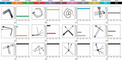
Based on the common movement patterns encountered in practice, 11 RDMP classes labeled from K1 to K11 are defined in this paper, including 10 regular classes: move straight, turn left, turn right, converge, diverge, cross, reverse, zigzag, clockwise, counter-clockwise and an 11th class called others. The last class covers all the other patterns that do not belong to K1-K10, e.g. background and noise. It is a common technique used in object detection to handle the case where the sliding window captures the background or part of a pattern (Ren et al. 2015). More details are described in Section 4.2. Several examples of movements in K1-K10 are displayed in Figure 2. It is important to mark that these definitions are highly fuzzy and conceptual, where noise in observations and a small proportion of irregular movements are tolerated.

Figure 2. Example of 10 classes of regular regional dominant movement patterns. The caption indicates class index and name.

4. TRNet for RDMP detection

In this section, the directional flow image is introduced first, followed by synthetic data generation. After that, the architecture of TRNet and RDMP detection are presented.

4.1. Directional flow image

Inspired by the histogram of oriented gradients (HOG) descriptor (Dalal and Triggs 2005), the directional flow image (DFI) is designed to capture both the position and direction information in a set of trajectories. In this section, a formal definition of DFI is given first followed by a detailed description of the DFI construction algorithm.

Given a set of trajectories $\mathcal{T}$, a DFI is defined as a $M$-channel image with a height of $H$ and width of $W$ (in unit of pixels), where each pixel stores the directional flows into its neighboring pixels. Let $g_{i,j}$ denote a pixel in DFI with a column index of $i$ ($i\in N^{+},1\le i\le W$) and row index of $j$ ($j\in N^{+},1\le j\le H$). An array of $M$ values is stored at $g_{i,j}$ written as:

(1) $I_{i,j}=[a_1,a_2,\cdots ,a_M]$(1)

The value $a_m$ stores the number of movements in $\mathcal{T}$ from the pixel $g_{i,j}$ to its neighboring pixel $g_{i^{\prime },j^{\prime }}$ in the direction $m$. Nine neighbors of a grid (including itself) are considered thus $M$ = 9. Given $g_{i,j}$ and $g_{i^{\prime },j^{\prime }}$, the direction $m$ is calculated as:

(2) $m=5-(j^{\prime }-j)\times 3+(i^{\prime }-i)$(2)

where $1\le m\le 9$. Figure 3(a) illustrates the mapping from direction $m$ to the relative position of $g_{i^{\prime },j^{\prime }}$ with respect to $g_{i,j}$. Direction 5 represents moving from one pixel to itself, which is assumed to mark the endpoint of a trajectory. Therefore, channel 5 of DFI stores the frequency of endpoints in each pixel.

Figure 3. Illustration of DFI generation. (a) the number in a grid represents the direction $m$ of $g_{i^{\prime },j^{\prime }}$ with respect to $g_{i,j}$ located at the centering grid (bold border); (b) selected pixel value of the DFI created from a single trajectory; (c) DFI of a K4-Converge pattern; (d) DFI of a K5-Diverge pattern. In (c) and (d), the nine channels of DFI are labeled from $I^1$ to $I^9$.

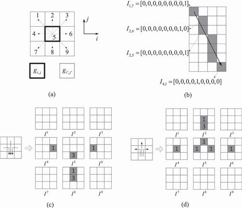
A concrete example is displayed in Figure 3(b) where a DFI of shape $9\times 7\times 4$ is generated from a single trajectory. The trajectory is firstly rasterized as a sequence of grids using Bresenham’s algorithm (Bresenham 1965). In the first pixel $g_{1,7}$, the object firstly moves to its neighboring pixel $g_{2,6}$ in direction 9 so that $I_{1,7}=[0,0,0,0,0,0,0,0,1]$. Subsequently, it moves from $g_{2,6}$ to $g_{2,5}$ in the direction 8, so that $I_{2,6}=[0,0,0,0,0,0,0,1,0]$. Finally, the object stops at the bottom right pixel, which is treated as moving from $g_{4,1}$ to itself. Therefore, the value is stored as $I_{4,1}=[0,0,0,0,1,0,0,0,0]$.

Each channel $I^m$ of DFI actually stores the flows in direction $m$ for $\mathcal{T}$. Two examples of DFI generated from a trajectory set are further provided in Figure 3(c, d) where the endpoints of the trajectories are stored in the channel $I^5$. It can be observed that the DFI generated from the converging and diverging trajectories are significantly different, which makes it possible to distinguish them.

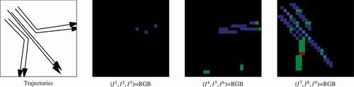
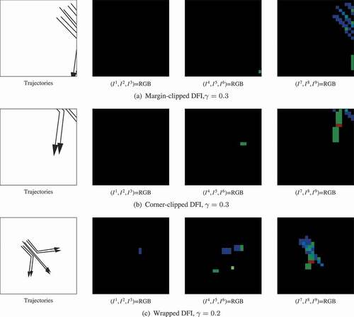
As a DFI contains nine channels, it can be visualized as three RGB images with each consecutive three channels of a DFI rendered as the red, green and blue band of an RGB image, respectively. An example is illustrated in Figure 4. Since most of the movement occurs in the direction 7, 8 and 9, the third RGB image shows more pixels in blue ($I^9$ channel) and green color ($I^8$ channel).

Figure 4. Visualization of DFI using three RGB images. Each consecutive three channels of DFI are rendered as the red, green and blue channel of one RGB file, respectively.

When constructing DFI from a trajectory set $\mathcal{T}$, the shape configuration of DFI needs to be determined first, which includes the coordinates of bottom left point of DFI denoted by $({\hat{x}}_{min},{\hat{y}}_{min})$, the size of a single grid $\delta$ (with equal width and height) and the width $W$ and height $H$ of DFI (in unit of grids). These parameters are determined based on user specification and the extent of input trajectory set $\mathcal{T}$. Let $(x_{min},y_{min},x_{max},y_{max})$ denote the minimum bounding rectangle (MBR) of $\mathcal{T}$, the shape configuration of DFI can be determined in two modes: fixed grid and fixed shape.

● fixed grid: the grid size $\delta$ is specified by the user while $({\hat{x}}_{min},{\hat{y}}_{min})$ and $(W,H)$ is calculated from the extent of $\mathcal{T}$ as:

(3) ${\hat{x}}_{min}=x_{min}-0.5\delta$(3)

(4) ${\hat{y}}_{min}=y_{min}-0.5\delta$(4)

(5) $W=\lfloor (x_{max}-x_{min})/\delta \rfloor +1$(5)

(6) $H=\lfloor (y_{max}-y_{min})/\delta \rfloor +1$(6)

where $\lfloor \rfloor$ represents the mathematical floor function. An example is illustrated in Figure 5(a).

Figure 5. Illustration of computing the shape configuration of DFI from the minimum bounding rectangle (MBR) of trajectories: fixed grid mode (a) and fixed shape mode (b,c). The dotted line represents the MBR of a trajectory set.

● fixed shape: the height $H$ and width $W$ of the DFI are specified by the user while $({\hat{x}}_{min},{\hat{y}}_{min})$ and $\delta$ is computed from the extent of $\mathcal{T}$. Analogously, we have

(7) $\delta =max(\frac{x_{max}-x_{min}}{W-1},\frac{y_{max}-y_{min}}{H-1})$(7)

(8) ${\hat{x}}_{min}=(x_{min}+x_{max}-W\delta )/2$(8)

(9) ${\hat{y}}_{min}=(y_{min}+y_{max}-H\delta )/2$(9)

Two examples of fixed shape mode are displayed in Figure 5(b,c). The DFI generated from a specific set of trajectories can vary with the shape of DFI specified. The fixed shape mode is primarily used in the synthetic data generation procedure where the trajectories are assured to have a square extent. Consequently, DFIs can be generated in uniform and square shape, which facilitates the training of TRNet. On the other hand, the fixed grid mode is adopted when generating DFI for a real-world trajectory dataset, whose shape is not known in advance.

After the shape configuration of DFI is determined, a DFI can be constructed from $\mathcal{T}$ following Algorithm 1. For each trajectory $\tau$ in $\mathcal{T}$, a sequence of grids $gridSeq$ passed by $\tau$ is obtained first by rasterizing $\tau$ using Bresenham’s algorithm (Bresenham 1965). Subsequently, $gridSeq$ is iterated where consecutive grids are examined with the directional flow information recorded in DFI. At the $n$th grid $gridSeq[n]$, the object moves from $gridSeq[n]$ to the next grid $gridSeq[n+1]$, the direction of movement $m$ is calculated according to Equation (2)(2) $m=5-(j^{\prime }-j)\times 3+(i^{\prime }-i)$(2) and the channel $m$ of the pixel corresponding to $gridSeq[n]$ in DFI is incremented as described by line 5 to 9 of Algorithm 5. For the last grid, only channel 5 is incremented. Finally, a DFI containing $M$ channels with the shape of $(W,H)$ is generated. The shape of DFI is written as $9\times H\times W$. In this paper, $M$ is set as $9$ and all the DFIs are created with a square shape where $H=W$. For simplicity, we directly refer to the shape of DFI as $D\times D$ where $D$ is the number of pixels in both height and width.

Algorithm 1: Directional flow image construction algorithm

Input:

$\mathcal{T}$: a trajectory set

${\hat{x}}_{min},{\hat{y}}_{min},\delta ,H,W$: shape configuration of DFI

Output

$\mathrm{I}$: a DFI of shape $9\times H\times W$

1 $\mathrm{I}$ = EmptyDFI($H,W$)

2 for $\tau$ in $\mathcal{T}$ do

3 gridSeq = BresenhamRasterize($tr,{\hat{x}}_{min},{\hat{y}}_{min},\delta$)

4 N = $|$gridSeq$|$

5 for n in 1 to N-1 do

6 $i$ = gridSeq[$n$].x, $j$ = gridSeq[$n$].y

7 $i^{\prime }$ = gridSeq[$n+1$].x, $j^{\prime }$ = gridSeq[$n+1$].y

8 $m=5-(j^{\prime }-j)\times 3+(i^{\prime }-i)$

9 $9{\mathrm{I}}_{i,j}^m+=1$

10 end

/*Update the pixel value of the last grid.

11 $i$ = gridSeq[N].x, $j$ = gridSeq[N].y

12 $12{\mathrm{I}}_{i,j}^5+=1$

13 end

14 return I

4.2. Synthetic data generation

The synthetic training data generation is divided into three steps. Firstly, trajectory seeds are drawn manually to follow these 10 RDMPs shown in Figure 2. Each seed is a set of trajectories following a specific RDMP. The definition of RDMP is highly fuzzy and conceptual. During the drawing of trajectory seed, different types of variations in a trajectory set are considered including the number of points inside a trajectory and the size of a trajectory set, as shown in Figure 1.

In practice, it is commonly required to detect RDMPs in a large set of trajectories, which could occur at multiple scales. A sliding window detection approach is adopted to address this problem by performing an exhaustive search in the space. More details are presented in Section 4.4. In that process, it is common to classify a DFI that differs significantly from those defined above. Therefore, an extra category labeled K11-Others is introduced to cover all other patterns that do not belong to the above 10 classes. Specifically, it contains two types of DFI: background and noisy. More details are presented below.

The background type corresponds to the case where only part of a trajectory set is covered by a window or the window is too large. Inspired by the anchor boxes used in Faster regional CNN (Ren et al. 2015), background DFI is generated by clipping a DFI in the K1-K10 category to generate a partially overlapped DFI. The clipping is controlled by the Intersection-over-Union (IoU) ratio. Let $b_1$ and $b_2$ denote two boxes, their IoU ratio denoted by $\gamma$ is calculated as:

(10) $\gamma =\mathrm{I}\mathrm{o}\mathrm{U}(b_1,b_2)=\frac{Area(b_1\cap b_2)}{Area(b_1\cup b_2)}$(10)

The clipping position can be set as either the margin or corner. Two examples are presented in Figure 6(a,b) where the DFI is generated by clipping the trajectory set shown in Figure 4. It could also happen that the area captured by the window is too large compared with the extent of a trajectory set. To take this factor into consideration, the extent of DFI can be enlarged under the control of $\gamma$. An example is illustrated in Figure 6(c). For generating a background DFI, $\gamma$ is empirically set as 0.3 for clipping along the margin and corner and 0.2 for enlarging the extent.

Figure 6. Illustration of generating background DFI in the K11-Others class by transforming the trajectory set in K5-Diverge class displayed in Figure 4.

The noisy type of DFI covers some other regular movement patterns which are encountered in real-world data but not defined here, e.g. T pattern. To represent these cases, trajectories are also drawn to follow some regular patterns beyond K1 to K10. Some examples can be found in the last row of Figure 9.

In the second step of synthetic data creation, data augmentation is performed by rotating these trajectory seeds to generates a larger number of trajectory sets. It is important to note that all the RDMP classes defined in this paper are rotation invariant. In other words, rotating $\mathcal{T}$ by an arbitrary angle does not change the category. Based on that property, synthetic labeled trajectories can be easily augmented. A trajectory group is drawn manually according to the specified category and serves as a seed. That seed is then rotated multiple times by $\alpha$ to generate $360/\alpha$ samples belonging to that category. When drawing these seeds, variations are imposed primarily on the number of trajectories, proportions of individual branches and angles of movement to minimize the redundancy in the training data.

In the final step, DFIs are generated from the trajectory sets. To investigate the influence of DFI shape on the training of TRNet, three shapes of DFI are generated in this paper: $10\times 10,25\times 25$ and $50\times 50$. For a single shape, the constitution of the synthetic dataset is reported in Table 1. For each class in K1-K10, 34 trajectory seeds are manually drawn and they are rotated by 30 degrees for data augmentation. Regarding the K11 class, a larger number of DFIs are created as K11 is supposed to cover all the other cases beyond K1 to K10. For the noisy movement, 44 trajectory seeds are firstly drawn manually and 528 trajectory sets are generated after performing the same augmentation of rotation. Moreover, 4080 background DFIs are generated by randomly collecting samples from the DFIs in K1-K10 and performing the clip and extent enlargement operation. These background DFIs comprise an equal number (1360) of margin-clipped, corner-clipped and extent-enlarged DFI illustrated in Figure 6. Finally, 8868 images are generated for a single DFI shape. Training of TRNet using the synthetic data is presented in Section 5.1.

Table 1. Synthetic data constitution for a particular shape of DFI.

	Number of trajectory sets
Class	Seed	After rotation	After clipping and wrapping	Number of DFIs
K1-K10	34	408	–	4080
K11(noise)	34	528	–	528
K11(background)	–	–	4080	4080
Sum	–	–	–	8688

4.3. Architecture design of TRNet

Inspired by LeNet that was originally designed for a handwritten digit recognition task (Lecun et al. 1998), TRNet is designed with several specific modifications described below.

In this paper, 11 classes of RDMP are considered where K11-Others is supposed to cover all the other cases beyond K1 to K10. Actually, there exists a hierarchical relationship where K1 to K10 constitute a regular class as a whole. That regular class together with K11-Others is supposed to fill the domain of DFI. To maximize the coverage of these relevant cases, many more samples are added to K11-Others than the remaining classes, as reported in Table 1. The imbalance of samples could cause a bias in training the classification model since more weight is put on the K11 class.

To alleviate this imbalance problem, TRNet is designed to contain two classifiers. The first one is a binary classifier, denoted by $C_b$, which determines whether the DFI belongs to the regular class (K1-K10) or not (K11). When training $C_b$, all the samples in K1 to K10 are relabeled as 0 to denote the regular class and these samples in K11 are relabeled as 1. After aggregating all the samples from K1 to K10, the two classes have almost the same number of samples as reported in Table 1. The second classifier is called a regular one denoted by $C_r$, which only distinguishes DFI from K1 to K10.

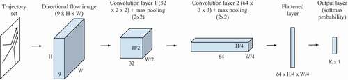
The two classifiers in TRNet are designed as two neural networks with the architecture shown in Figure 7. Each network is created separately to take a DFI of shape $9\times H\times W$ as input. A convolution layer with 32 filters in size of $3\times 3$ is added to extract features from the DFI. That convolution layer is then connected with a maximum pooling layer which reduces the size of the feature map by a factor of 2. A second group of convolution layer with 64 filters and maximum pooling layer is then appended to the network. The last pooling layer is then flattened and fully connected with a softmax probability layer of shape $K\times 1$, where $K=2$ for the $C_b$ and $K=10$ for $C_r$. The output of the classifier is a vector with a length of $K$ indicating the probability of the DFI in each class.

Figure 7. Architecture of classifiers in TRNet. For the binary classifier $K=2$ and for the normal classifier $K=10$.

When a new DFI is classified, its label is determined by $C_b$ and $C_r$ collectively following Algorithm 2. Let $k_b,p_b$ and $k_r,p_r$ denote the class label and softmax probability return by $C_b$ and $C_r$ respectively. If the binary classifier $M_b$returns a label of 1 (corresponding to K11 class), and its probability $p_b$ is higher than $p_r$, the DFI is predicted as K11 with a probability of $p_b$; otherwise, it is predicted to be class $k_r$ with a probability of $p_r$.

Algorithm 2: Classify a DFI using the binary and regular classifier

Input:

$I$: A DFI to be classified

$C_b,C_r$: the binary and regular classifier

Output

$k$, $p$: the class label (1 to 11) and its the probability

/*k_b is 0 (regular) or 1 (others)*\

1 $k_b,p_b$: = $C_b$.classify(I)

/*k_r is in 1 or 10.*

2 $k_r,p_r$: = $C_r$.classify(I)

3 if $p_b>p_r$ and $k_b==1$ then

4 return 11, $p_b$

5 else

6 return $k_r$, $p_r$

7 end

The two classifiers are trained separately. The samples in K11 are only used for training of $C_b$ whereas the remaining samples are used in the training of both classifiers. For each classifier, the corresponding DFI samples are split into a training and a test subset. The former is used for training the model whereas the accuracy is reported on the latter. The loss function of TRNet is selected as a categorical cross-entropy measuring the difference between two distributions. It is calculated as:

(11) $L=-\frac{1}{N_{train}}\sum _i^{N_{train}}\sum _k^{K}p(x_i{)}_{k}log(q(x_i{)}_k)$(11)

where $N_{train}$ is the size of the training subset, $p(x_i{)}_k$ and $q(x_i{)}_k$ are the true and predicted probability of class $k$ for the training sample $x_i$. In the training process, $L$ is minimized using the ADADELTA gradient descent method (Zeiler 2012). The accuracy of the test subset is calculated as:

(12) $r_{test}=\frac{1}{N_{test}}\sum _i^{N_{test}}\varphi (y_i={\hat{y}}_i)$(12)

where $y_i$ is the true label of $i$th sample in the test dataset with the size of $N_{test}$, ${\hat{y}}_i$ is its predicted class and $\varphi (x)$ is an indicator function that returns 1 if the condition $x$ is true and 0 otherwise. The accuracy measures the generalization error of the trained model. In this paper, the DFI generation algorithm is implemented in C++ and TRNet is implemented in Python using the Keras library¹.

4.4. RDMP detection with TRNet

The objective of RDMP detection is to find the regions for the occurrence of specific RDMPs. In practice, RDMPs could occur at multiple scales when the trajectory data covers a large area, e.g. a city. To discover RDMPs at multiple scales, TRNet is treated as a classifier and a classical sliding window detection method is employed to exhaustively search over sub-regions of the DFI. One problem remains to be addressed that conventional CNN model can only accept image with fixed shape as input but the sub-regions can have a variable extent.

One strategy is generating an extremely large DFI for the whole study area and classifying regions in different sizes using a more advanced CNN model that can take an image of variable shape as input. For instance, He et al. (2015) designed a spatial pyramid pooling (SPP) layer to build a fixed-length vector from a variable shape of the convolutional feature map. With the SPP layer added, the CNN model still needs to be trained with images of different shapes. However, that approach is inappropriate for the RDMP detection as DFI shape can vary in a much broader range. Given a DFI generated with a grid size of 10 m, detecting RDMP in range of 100 m, 1k m and 10 km requires generating DFI of shape 10, 100 and 1000, respectively. The last size is too large to be used in the training procedure. As a consequence, the model could be problematic in detecting RDMPs in a 10 km range.

To address this problem, this paper adopts a different strategy. Instead of generating a single DFI and adopting advanced CNN models to handle DFI of variable shape, we generate a pyramid of DFIs at multiple scales with various grid sizes and apply the same conventional CNN model that takes DFI of a fixed shape as input. In the same example, we can train TRNet with DFIs of shape 10 and generate DFIs in a grid size of 10 m, 100 m and 1 km, respectively. The benefit is that the model can be trained in a memory-efficient way and RDMP can also be detected at multiple scales. The detailed approach is formally presented below.

Given a TRNet which takes input from DFI of shape $D\times D$ and a user-specified range of region sizes (in meters) denoted by $\mathcal{S}=[S_1,S_2,S_3,\cdots ,S_M]$, the RDMP detection procedure consists of the following steps:

1. Calculate a sequence of the grid sizes as $\mathrm{\Delta }=[{\delta }_1,{\delta }_2,\cdots ,{\delta }_M]$ where ${\delta }_m=S_m/D$. Create an empty set of boxes $B$ to store the detection result.

2. For each grid size ${\delta }_m$ in $\mathrm{\Delta }$, perform the following steps:

• (a) Generate a single DFI for the whole trajectory set $\mathcal{T}$ in fixed grid mode with grid size ${\delta }_m$;

• (b) Slide a window over the DFI with stride of $\lfloor r\cdot D\rfloor$ to examine sub-regions of the DFI, where $r$ is the stride ratio (empirically set as 0.2 in this paper). For a specific window with location denoted by a box $b$

(i). Normalize the extracted DFI and classify it with the TRNet;

(ii). Filter out $b$ if any of the two conditions are fulfilled: (a) the maximal softmax probability $p_m<\alpha$ where $\alpha$ is a user-specified threshold; (b) the DFI is classified as the K11-others category; otherwise export $b$ to $B$;

• (3) Merge the redundant boxes in $B$ and return a set of polygons $\mathcal{R}$ as the detection result. More details are presented below.

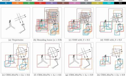
In sliding window detection, it is common to generate a large number of redundant boxes that actually identify the same object as shown in Figure 8. That problem is commonly handled in the previous work with a procedure called non-maximum suppression (NMS), which was originally developed for eliminating unwanted responses in edge detector (Prince 2012).

Figure 8. Illustration of non-maximum suppression (NMS) and clustering-based merging (CBM). The detected window sizes are set as $20\mathrm{\%},40\mathrm{\%},80\mathrm{\%}$ of $x_{max}-x_{min}$. The results of NMS and CBM are demonstrated in (c,d) and (e–h) respectively.

Let $B_k$ denote all the boxes classified as class $k$. The standard procedure of NMS is described below:

1. Select the box with the largest probability in $B_k$, denoted by $\hat{b}$;

2. Remove all the boxes in $B_k$ that intersects $\hat{b}$ with an IoU ratio higher than a threshold $\beta$;

3. Export $\hat{b}$ and return to step 1 until $B_k$ is empty.

An example of detecting RDMP in a region containing multiple RDMPs is demonstrated in Figure 8. After filtered by $\alpha =0.9$, the detected boxes are shown in Figure 8(b). It demonstrates that TRNet is effective in classifying RDMP in trajectories using DFI. However, the boxes are heavily overlapped and contain a lot of redundancy. The results of NMS pruning are displayed in Figure 8(c,d) where more boxes are pruned by a smaller $\beta$. However, the results are still problematic in several aspects. It cannot effectively prune the boxes in the same category but with a different size. NMS only considers the probability of prediction in pruning, which cannot eliminate these RDMPs that are part of others. In Figure 8(d), parts of a K2-Turn-Left pattern are detected as K1-Move-Straight.

Based on the above observation, a clustering-based merging (CBM) is developed in this paper to eliminate the redundant detection boxes in the following steps:

1. Cluster the boxes $B_k$ using DBSCAN (Ester et al. 1996) by specifying the distance threshold $\epsilon$ and the minimum size of cluster $MinPts$. The distance between the two boxes $b_1,b_2$ is calculated as:

(13) $dist(b_1,b_2)=1-\mathrm{I}\mathrm{o}\mathrm{U}(b_1,b_2)$(13)

It measures the spatial closeness between two boxes, which is in a range of [0,1]. The distance of two disjoint boxes is 1 and that of two identical boxes is 0.

• (2) For each cluster, generate the cascaded union of the boxes as a polygon $R$. Export $(R,k)$ to the result $\mathcal{R}$.

As each polygon in $\mathcal{R}$ is generated as a cascaded union of neighboring boxes in the same class, the restriction imposed by the square shape of the detection window can be partly relaxed.

The result of CBM is illustrated in Figure 8(e–f). With too small $\epsilon$, boxes in the same category but with different sizes cannot be clustered properly, as demonstrated by the K2 and K5 boxes in Figure 8(e,f). When $MinPts$ is too small, some embedded RDMPs will form a cluster and cannot be pruned, as shown by the K1 boxes in Figure 8(h). However, setting a large $MinPts$ may prune the boxes that should have been kept. For example, the K2 box in (e) is pruned in (f) by setting a larger $MinPts$. In Figure 8(g), it shows that with the proper setting of $MinPts$ and $\epsilon$, the redundancy in the detection results can be effectively eliminated. The result displayed in Figure 8 also implies that the selection of CBM parameters could be influenced by the spatial distribution of RDMPs. In practice, a small region could be selected to explore these parameters before applying them to the whole study area.

5. Experiments

5.1. Training of TRNet

The synthetic dataset is created to contain DFIs in three shapes $10\times 10$, $25\times 25$ and $50\times 50$. According to the statistics shown in Table 1, 8868 images are generated for each shape. For the training of the binary classifier, all the samples are randomly split into a training subset 70% (6208 samples) and a test subset 30% (2660 samples). For the training of the regular 10-class classifier, the 4080 samples from K1 to K10 are used with the same split ratio of training (2856 samples) and test subset (1224 samples).

The accuracy and training time of different classifiers are reported in Table 2. To compare the training result without handling the class imbalance problem described in Section 4.3, another 11-class classifier is trained in the same architecture shown in Figure 7 with $K=11$. It can be observed that the regular classifier achieves the highest accuracy close to 100% for all the three shapes of DFI. The accuracy of the binary classifier is significantly smaller than the regular one but much higher than the 11-class classifier. The reason could be that these 10 classes from K1 to K10 are highly distinguishable from each other so that they can be easily separated by the model. Although the binary classifier only needs to distinguish two classes, the diversity of its training samples substantially increases after adding samples in the K11 class. Consequently, it becomes difficult to train the binary classifier to learn these complex patterns and the case is even worse for the 11-class classifier. After combining the binary and regular classifier, the final accuracy is still higher than the 11-class one, which demonstrates the effectiveness of training two classifiers to address the class imbalance problem.

Table 2. Comparison of accuracy and training time for different classifiers. The training process contains 100 epochs.

DFI shape (D)	Classifier	Average accuracy (%)	Training time (seconds)
10	Binary (K =2)	94.28	36.48
	Regular (K =10)	99.30	25.57
	Binary + Regular (K = 11)	96.65	–
	11-class (K = 11)	88.12	37.75
25	Binary (K =2)	93.37	63.76
	Regular (K =10)	99.59	43.08
	Binary + Regular (K = 11)	94.49	–
	11-class classifer (K = 11)	87.94	64.17
50	Binary (K =2)	91.44	159.42
	Regular (K =10)	100.00	103.04
	Binary + Regular (K = 11)	92.73	–
	11-class classifer (K = 11)	80.89	167.42

Another interesting observation in Table 2 is that a larger DFI shape tends to slightly decrease the accuracy of these classifiers. The reason can be explained in two ways. When the shape of DFI increases, its domain also becomes larger and it could be more difficult to learn these complex patterns. The features captured by DFI store more precise movement information at a microscopic scale, which could distract the model from learning these macroscopic patterns.

More concrete examples of the classification result are displayed in Figure 9, where DFI is generated from the trajectories in a fixed shape of $10\times 10$. It can be observed from the first row that TRNet can effectively classify the RDMP in a trajectory set, which is also robust to different kinds of noise and variations. When there exists a large deviation from a standard RDMP, the maximum softmax probability predicted by TRNet decreases, as shown in the second row of Figure 9. Some patterns manually labeled as the category K11-Others can also be classified correctly, e.g. T pattern in Figure 9(i). In Figure 9(g), there exists a mixture of turning left and diverging pattern whereas the former is dominant. Consequently, the predicted probability of K2 is higher than K5.

Figure 9. Some classification results of TRNet with DFI generated in shape of $10\times 10$. The trajectories are shown on the left side and the softmax probabilities are shown on the right.

5.2. Case study

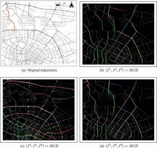
After trained on the synthetic dataset, TRNet is evaluated on a public real-world taxi GPS dataset collected by DiDiChuXing, a taxi-requesting company in China². The data covers an area of shape 8.8 km $\times$ 7.5 km in Chengdu, China. The GPS observations are collected every 3 s on average, where taxi order ID, vehicle ID, location and timestamp are recorded. The original data are collected for a 1-month period with 30 million observations per day on average. In this paper, only 1 day’s data (2016-11-01) are analyzed for demonstration purpose.

Figure 10 presents a map for the trajectories collected from 8:00 am to 9:00 am and the corresponding DFI. Some knowledge of the underlying movement can already be obtained from the visualization of DFI. It is reasonable to observe that most of the colors match with the direction of the underlying roads where the movement is constrained. For instance, the green color in Figure 10(b) indicates a high value in the channel $I^2$, which implies a high volume of flow in the north direction. Additionally, several roads in the northwestern direction are highlighted in Figure 10(b). In most of these places, green color can be observed in Figure 10(d), which corresponds to the channel $I^8$. It indicates that these roads also have a high volume in the southern direction. In Figure 10(c), the green color presents the distribution of the last point of these trajectories, namely, the destination of trips. However, visual inspection of DFI is still limited in discovering more complex movement patterns, where RDMP detection is needed.

Figure 10. DFI generated from real-world taxi trajectories. (a) Original trajectories collected from 8:00 to 9:00 am in Chengdu where a single trajectory is highlighted for illustration. (b–d) Visualization of DFI. The channels $I^1$ to $I^3$, $I^4$ to $I^6$ and $I^7$ to $I^9$ are rendered as an RGB image, respectively. The grid size is specified as 50 m.

5.2.1. RDMP detection results

According to the statistics reported in Table 2, TRNet with DFI shape of 10 is adopted for RDMP detection as it achieves the highest accuracy.

In the first experiment, sliding window detection is evaluated using trajectories collected from 8:00 to 8:05 am with the region size empirically set as $\mathcal{S}=[250m,500m,1km,2.5km]$. The result is displayed in Figure 11. It can be observed that a large proportion of boxes are classified as K7-Reverse and K6-Cross. It can be explained by the fact that vehicle movement is primarily constrained to the road network which contains a lot of bidirectional roads and intersections. K2-Turn-Left and K5-Diverge are also frequently detected at some specific intersections. K8-Zigzag accounts for the smallest proportion as vehicles rarely move in that manner. Another interesting observation is that large boxes are concentrated on the class K6 and K7. The reason could be that a larger region tends to capture more objects, which is less likely to exhibit a dominant movement pattern. However, the high volume of flows at bidirectional roads and intersections could still be dominant.

Figure 11. Sensitivity analysis of sliding window detection results with respect to the probability threshold $\alpha$ and stride ratio $r$. The trajectories are collected from 8:00 to 8:05 am. The other configurations are set as $D=10,\mathcal{S}=[250m,500m,1km,2.5km]$. The three columns show RDMPs detected in K1-K5 (left), K7 (middle) and K6,K8-K10 (right).

The sensitivity of sliding window detection results with respect to the probability threshold $\alpha$ and stride ratio $r$ can be inspected by comparing these maps in Figure 11. It is expected to detect more boxes with a smaller $\alpha$. In addition, fewer boxes are detected with a larger $r$, where a smaller number of boxes are examined in the sliding window detection step. However, there are still many boxes that are only detected with $r=0.2$. That observation reveals a significant difference between RDMP detection and conventional object detection problems. RDMP detection is much more sensitive to the boundary of the sliding window as the movement recorded does not cover a continuous region in the space. Taking the trajectories displayed in Figure 9(e) as an example, if the detection window is shifted a little towards the bottom then a K1-Move-Straight pattern will be detected. Therefore, it is more likely to miss some patterns with a larger stride ratio $r$.

The second experiment investigates the sensitivity of CBM with respect to configurations of $MinPts$ and $\epsilon$. The other configurations are set as $D=10,\alpha =0.9,r=0.2$ and $\mathcal{S}=[250m,500m,1km,2.5km]$. The result is depicted in Figure 12. CBM can effectively eliminate the redundancy in the result of sliding window detection shown in Figure 11. With a larger $MinPts$, patterns spreading a wider region can be discovered. On the other hand, the region of a pattern can be more accurately identified with a smaller $\epsilon$. These maps also provide a clear view of the distribution of RDMPs. K1-Move-Straight patterns are majorly discovered at the roads with the flow in a single direction. K6-Cross and K7-Reverse are widely distributed in the area. K9-Clockwise and K10-Counter-Clockwise are discovered at these roads with a large curvature. K5-Diverge is concentrated on the southern region of the city where the road density is also higher.

Figure 12. Sensitivity analysis of clustering based merging (CBM) results with respect to configurations of $MinPts$ and $\epsilon$. The trajectories are collected from 8:00 to 8:05 am. The other configurations are set as $D=10,\mathcal{S}=[250m,500m,1km,2.5km],\alpha =0.9,r=0.2$. The three columns show RDMPs detected in K1-K5 (left), K7 (middle) and K6,K8-K10 (right).

In the third experiment, temporal variations of RDMPs are explored by comparing RDMPs detected in a 30-min period in the morning, noon and afternoon. The configurations are set as $D=10,\alpha =0.9,r=0.2,\mathcal{S}=[250m,500m,1km,2.5km],MinPts=4$ and $\epsilon =0.6$. The result is demonstrated in Figure 13. Several places with a stable movement pattern can be identified by comparing the maps in the left column. A K3-Turn-right pattern is detected at one intersection in the northern region of the city in all the three periods. In the northwestern region, a Y-shape intersection is detected as K5-Diverge pattern and another T-shape intersection as K4-Converge pattern. Several roads in the north-west direction in the western region are detected as K1-Move-Straight pattern. In the eastern region, the K4-Converge pattern is observed in the afternoon as opposed to K3-Turn-right in the noon and K1-Move-Straight in the morning. The maps in the middle column show that fewer K7-Reverse patterns are observed in the noon than the other two periods. Additionally, fewer K6-Cross patterns are observed in the noon and afternoon than the morning.

Figure 13. Comparison of RDMPs detected a 30-min time period in the morning (a), noon (b) and afternoon (c). The configurations are set as $D=10,\mathcal{S}=[250m,500m,1km,2.5km],\alpha =0.9,r=0.2,MinPts=4$ and $\epsilon =0.6$.

5.2.2. Performance analysis

The running time of some selected configurations of RDMP detection is reported in Table 3. As can be observed, the performance of RDMP detection substantially decreases with the increase of DFI shape $D$ and the reduction of stride ratio $r$. On the other hand, the size of trajectory set exhibits a relatively small effect on the total running time.

Table 3. Running time of RDMP detection. The detection configurations are set as $\alpha =0.9,MinPts=4,\epsilon =0.6,\mathcal{S}=[250m,500m,1km,2.5km]$. The symbol $D$ represents DFI shape and $r$ is the stride ratio used in sliding window detection.

				Running time (seconds)
Data collection period	$|\mathcal{T}|$	$D$	$r$	DFI generation	Sliding window detection	CBM pruning	Total
8:00–8:05 am	2270	$10$	0.2	0.892	15.312	3.959	20.163
8:00–8:05 am	2270	$10$	0.3	0.892	6.722	3.765	11.379
8:00–8:05 am	2270	$25$	0.2	0.906	47.499	4.186	52.591
8:00–8:05 am	2270	$50$	0.2	0.924	158.095	4.210	163.229
8:00–8:30 am	9169	$10$	0.2	2.105	17.003	4.372	23.480
8:00–9:00 am	15,729	$10$	0.2	3.671	17.356	4.532	25.559
12:00–12:30 am	9753	$10$	0.2	1.949	17.353	4.806	24.108
17:00–17:30 am	11,567	$10$	0.2	2.550	17.279	4.574	24.403

The bottleneck of the RDMP detection program lies in the sliding window detection step, where subregions of the DFI are extracted and classified by TRNet. When the DFI shape $D$ increases from 10 to 50, the running time of the sliding window step increases by 9 times. The reason is that the image extracted for each subregion consumes much higher memory. Consequently, both retrieving subregions from a large DFI and classifying these images take a longer time. With a smaller $r$, a larger number of windows need to be examined, which also degrades the performance.

The impact of trajectory set size $|\mathcal{T}|$ on the performance is relatively small because the shape of DFI is only determined by the extent of the trajectories. Although the running time of DFI generation linearly increases with $|\mathcal{T}|$, it is still the smallest one among the three steps. The running time of CBS pruning is relatively consistent with respect to DFI shape and trajectory set size, which is primarily influenced by the number of RDMPs detected.

The above comparison further implies that the proposed method has a high scalability with respect to data volume. However, it may not be scale well to a large study area if many RDMPs occur on a small scale. In that case, the number of windows to be examined considerably increases. Addressing that type of scalability problem will be left as a future work.

6. Conclusions and future work

In this paper, a deep learning approach was proposed to find the regions where a specific RDMP occurs in a large collection of trajectories. A novel feature descriptor for a trajectory set was first proposed as a directional flow image, which stores the flow information from each pixel to its neighboring pixels. A classification model called TRNet was designed based on CNN, which contains a binary classifier for identifying the background and noisy RDMP and a 10-class classifier for distinguishing 10 commonly encountered RDMPs in the real world. A synthetic trajectory dataset was created by manually drawing trajectories to follow these RDMPs and training of TRNet achieved considerably high accuracy. Detecting RDMPs at multiple scales was solved by a sliding window detector and clustering-based merging suppression. Experiments on a real-world taxi trajectory dataset demonstrated that the proposed approach can effectively and efficiently detect a wide range of RDMPs in a large collection of trajectories. The approach also provided a guideline for applying deep learning approaches to movement pattern analysis.

Although only 11 classes of RDMP are considered in this paper, the proposed model can be easily extended to detect other types of patterns by enlarging the training dataset. Trajectory seeds in user-specified class (e.g. T pattern) can be added to retrain the model. Alternatively, the current classification scheme can be expanded by dividing one class into more specific classes. For instance, K1-Move-Straight samples can be relabeled as moving towards the north or south. It would also be possible to discover regular movement patterns by performing unsupervised learning such as clustering on the DFIs extracted from various time periods. However, some issues still exist in the performance and robustness to geometric transformations. We will leave these tasks as future work.

In addition to detecting other types of movement patterns, the proposed approach can be improved in several ways. First, the current approach can only find the regions where a specific pattern occurs whereas it remains unknown about which group of trajectories actually follows that pattern. One potential solution is to retrieve and analyze the trajectories passing through the detected regions, which will be explored in the future. Second, DFI is extracted as a nine-channel image, which can be highly sparse as the movement patterns, in reality, may only occupy a rather small subspace of the DFI domain. Reducing the dimension of DFI to save memory and improve performance is another research direction. Third, the current model can further be evaluated on other types of movement data such as the immigration track of animals.

Acknowledgments

The authors would like to acknowledge the editor and the anonymous three reviewers for their valuable suggestions. The first author is supported by the Chinese Scholarship Council. The project is also partly funded by the strategic project RENO financed by the Integrated Transport Research Lab (ITRL) at KTH.

Disclosure statement

No potential conflict of interest was reported by the authors.

Data and codes availability statement

The data and codes that support the findings of this study are available in zenodo repository with the identifier doi:10.5281/zenodo.3530373.

Additional information

Notes on contributors

Can Yang

Can Yang is a Ph.D. student in the Department of Urban Planning and Environment at KTH, Royal Institute of Technology in Sweden. His research interests include spatio-temporal data mining, movement pattern analysis and map matching.

Győző Gidófalvi

Győző Gidófalvi is an associate professor in the Department of Urban Planning and Environment at KTH, Royal Institute of Technology in Sweden. His research interests include spatio-temporal data mining and analysis, location-based services, locations privacy and intelligent transportation systems.

Notes

1. https://github.com/keras-team/keras.

2. The data can be downloaded at https://outreach.didichuxing.com/research/opendata/en/.

References

- Belongie, S., Malik, J., and Puzicha, J., 2002. Shape matching and object recognition using shape contexts. IEEE Transactions on Pattern Analysis and Machine Intelligence, 24 (4), 509–522. doi:10.1109/34.993558
- Bogorny, V., Kuijpers, B., and Alvares, L.O., 2009. ST-DMQL: a semantic trajectory data mining query language. International Journal of Geographical Information Science, 23 (10), 1245–1276. doi:10.1080/13658810802231449
- Bresenham, J.E., 1965. Algorithm for computer control of a digital plotter. IBM Systems Journal, 4 (1), 25–30. doi:10.1147/sj.41.0025
- Cao, H., Mamoulis, N., and Cheung, D.W., 2005. Mining frequent spatio-temporal sequential patterns. In: Proceedings - IEEE international conference on data mining, ICDM, 82–89. doi:10.1016/j.chroma.2005.02.027
- Choi, D.W., Pei, J., and Heinis, T., 2017. Efficient mining of regional movement patterns in semantic trajectories. Proceedings of the VLDB Endowment, 10 (13), 2073–2084. doi:10.14778/3151106.3151111
- Dalal, N. and Triggs, B., 2005. Histograms of oriented gradients for human detection. In: Proceedings of the 2005 IEEE computer society conference on computer vision and pattern recognition (CVPR’05) - Volume 1 - Volume 01, CVPR ’05. Washington, DC: IEEE Computer Society, 886–893. doi:10.1213/01.ANE.0000159168.69934.CC
- De Lucca Siqueira, F. and Bogorny, V., 2011. Discovering chasing behavior in moving object trajectories. Transactions in GIS, 15 (5), 667–688. doi:10.1111/tgis.2011.15.issue-5
- Demšar, U. and Virrantaus, K., 2010. Space–time density of trajectories: exploring spatio-temporal patterns in movement data. International Journal of Geographical Information Science, 24 (10), 1527–1542. doi:10.1080/13658816.2010.511223
- Dodge, S., Weibel, R., and Lautenschütz, A.K., 2008. Towards a taxonomy of movement patterns. Information Visualization, 7 (April), 240–252. doi:10.1057/PALGRAVE.IVS.9500182
- Endo, Y., et al. 2016. Classifying spatial trajectories using representation learning. International Journal of Data Science and Analytics, 2 (3), 107–117. doi:10.1007/s41060-016-0014-1
- Ester, M., et al., 1996. A density-based algorithm for discovering clusters a density-based algorithm for discovering clusters in large spatial databases with noise. In: Proceedings of the second international conference on knowledge discovery and data mining, KDD’96. Portland: Oregon AAAI Press, 226–231.
- Graves, A., Mohamed, A.R., and Hinton, G., 2013. Speech recognition with deep recurrent neural networks. In: 2013 IEEE international conference on acoustics, speech and signal processing, May Vancouver, BC. Canada: IEEE, 6645–6649.
- Guo, D., et al., 2012. Discovering spatial patterns in origin-destination mobility data. Transactions in GIS, 16 (3), 411–429. doi:10.1111/tgis.2012.16.issue-3
- He, K., et al., 2015. Spatial pyramid pooling in deep convolutional networks for visual recognition. IEEE Transactions on Pattern Analysis and Machine Intelligence, 37 (9), 1904–1916. doi:10.1109/TPAMI.2015.2389824
- Hinton, G.E., Osindero, S., and Teh, Y.W., 2006. A fast learning algorithm for deep belief nets. Neural Computation, 18 (7), 1527–1554. doi:10.1162/neco.2006.18.7.1527
- Karpathy, A., et al., 2014. Large-scale video classification with convolutional neural networks. In: Proceedings of the 2014 IEEE conference on computer vision and pattern recognition, CVPR ’14. Washington, DC: IEEE Computer Society, 1725–1732. doi:10.1007/s00330-014-3197-7
- Kim, Y., 2014. Convolutional neural networks for sentence classification. CoRR, computing research repository, abs/1408.5882.
- Krizhevsky, A., Sutskever, I., and Hinton, G.E., 2012. ImageNet classification with deep convolutional neural networks. In: Proceedings of the 25th international conference on neural information processing systems - Volume 1, NIPS’12. Lake Tahoe, Nevada: Curran Associates Inc, 1097–1105.
- Laube, P., Imfeld, S., and Weibel, R., 2005. Discovering relative motion patterns in groups of moving point objects. International Journal of Geographical Information Science, 19 (6), 639–668. doi:10.1080/13658810500105572
- Lecun, Y., et al., 1998. Gradient-based learning applied to document recognition. In: Proceedings of the IEEE, 2278–2324.
- Lee, J.G., Han, J., and Li, X., 2015. A unifying framework of mining trajectory patterns of various temporal tightness. IEEE Transactions on Knowledge and Data Engineering, 27 (6), 1478–1490. doi:10.1109/TKDE.2014.2377742
- Li, B., et al., 2011. Hunting or waiting? Discovering passenger-finding strategies from a large-scale real-world taxi dataset. In: 2011 IEEE international conference on pervasive computing and communications workshops (PERCOM Workshops), March, 63–68. doi:10.1016/j.tvjl.2010.05.029
- Li, Z., Wu, F., and Crofoot, M.C., 2013. Mining following relationships in movement data. In: 2013 IEEE 13th international conference on data mining (ICDM), 458–467.
- Mikolov, T., et al., 2010. Recurrent neural network based language model. In: Eleventh annual conference of the international speech communication association, Chiba, Japan.
- Prince, S.J.D., 2012. Computer vision: models, learning, and inference. 1st ed. New York, NY: Cambridge University Press.
- Ren, S., et al., 2015. Faster r-cnn: towards real-time object detection with region proposal networks. In: Advances in neural information processing systems, Montreal, Canada, 91–99.
- Shu, X. and Wu, X.J., 2011. A novel contour descriptor for 2D shape matching and its application to image retrieval. Image and Vision Computing, 29 (4), 286–294. doi:10.1016/j.imavis.2010.11.001
- Wachowicz, M., et al. 2011. Finding moving flock patterns among pedestrians through collective coherence. International Journal of Geographical Information Science, 25 (11), 1849–1864. doi:10.1080/13658816.2011.561209
- Wang, D., et al., 2017a. DeepSD: supply-demand prediction for online car-hailing services using deep neural networks. In: 2017 IEEE 33rd international conference on data engineering (ICDE), April, San Diego, California, 243–254.
- Wang, J., et al., 2017b. Automatic intersection and traffic rule detection by mining motor-vehicle GPS trajectories. Computers, Environment and Urban Systems, 64, 19–29. doi:10.1016/j.compenvurbsys.2016.12.006
- Wang, X., et al. 2014. Bag of contour fragments for robust shape classification. Pattern Recognition, 47 (6), 2116–2125. doi:10.1016/j.patcog.2013.12.008
- Xu, C., Liu, J., and Tang, X., 2009. 2D shape matching by contour flexibility. IEEE Transactions on Pattern Analysis and Machine Intelligence, 31 (1), 180–186. doi:10.1109/TPAMI.2008.199
- Yang, C. and Gidfalvi, G., 2018. Mining and visual exploration of closed contiguous sequential patterns in trajectories. International Journal of Geographical Information Science, 32 (7), 1282–1304. doi:10.1080/13658816.2017.1393542
- Yao, D., et al., 2017. Trajectory clustering via deep representation learning. In: 2017 International Joint Conference on Neural Networks (IJCNN), Anchorage, AK, 3880–3887.
- Yao, H., et al., 2018. Deep multi-view spatial-temporal network for taxi demand prediction. In: AAAI conference on artificial intelligence, New Orleans, Louisiana.
- Ye, Y., et al., 2009. Mining individual life pattern based on location history. In: 2009 Tenth international conference on mobile data management: systems, services and middleware IEEE, Taipei, Taiwan, 1–10.
- Zeiler, M.D., 2012. ADADELTA: an adaptive learning rate method. CoRR, computing research repository, abs/1212.5701. doi:10.1094/PDIS-11-11-0999-PDN
- Zhang, J., Zheng, Y., and Qi, D., 2017. Deep spatio-temporal residual networks for citywide crowd flows prediction. In: AAAI conference on artificial intelligence, San Francisco, California, 1655–1661.