A distributed framework for extracting maritime traffic patterns

ABSTRACT

All the modern surveillance systems take advantage of the Automatic Identification System (AIS), a compulsory tracking system for many types of vessels. Ships that carry AIS transponders on board transmit their position and status in order to alert nearby vessels and ground stations, but this information can well be used to identify events of interest and support decision making. The detection of anomalies (i.e. unexpected sailing behavior) in vessels’ trajectories is such an event, which is of utmost importance. Approaches for detecting such anomalies vary from extracting normality models to searching for individual cases, such as AIS switch-off or collision avoidance maneuvers. The current research work follows the former method; it employs sparse historic AIS data and polynomial interpolation in order to extract shipping lanes. It modifies the DB-Scan clustering algorithm in order to achieve more coherent trajectory clusters, which are then composed to create the shipping lanes. The proposed approach implements distributed processing on Apache Spark in order to improve processing speed and scalability and is evaluated using real-world AIS data collected from terrestrial AIS receivers. The evaluation shows that the biggest part (i.e. more than 90%) of any future vessel trajectory falls within the extracted shipping lanes.

KEYWORDS:

• Trajectory clustering
• AIS vessel monitoring
• anomaly detection
• distributed processing

1. Introduction

Despite the importance of maritime surveillance for the safety of passengers, vessels and their cargo, it was only since July 2002, when the Regulation 19 of the International Convention for the Safety of Life at Sea (SOLAS-V) came into force, that large cargo vessels are obliged to fit and use AIS for reporting their position, speed and heading, for serving surveillance purposes. This regulation resulted in an abundance of data that completely changed the maritime surveillance scenario. AIS transponders are today used also by smaller vessels, such as yachts or fishing boats (Montewka et al. (2009), that transmit their position and route to nearby vessels in order to avoid collisions. Additional data, concerning the vessel’s origin and destination, its type, size and draught are also periodically transmitted by AIS equipped vessels, thus providing a rich data set for further analysis.

In this direction maritime authorities can use this data for tracking vessels and analysing their behavior in order to early detect abnormalities, which may happen due to an engine failure, an accident in the sea, or on purpose. Building on the ideas of previous works in the field of anomalous vessel behaviour detection (Varlamis et al. 2019, Kontopoulos et al. 2019), this work focuses on the extraction of traffic patterns, which can be the basis for detecting such behaviours.

In this work, we extend Kontopoulos et al. (2019) by employing concepts of the network abstraction model proposed in Varlamis et al. (2019) and develop a methodology for processing multi-vessel AIS data more efficiently, using richer information on the network edges. The new network abstraction aims to extract multiple movement patterns for the same network edge, which correspond to a fine-grained clustering of the collected AIS data. Using Lagrange interpolation for adding intermediate points to the vessel trajectories improves the performance of the clustering algorithm Kontopoulos et al. (2020). The algorithm parameters are fine-tuned by considering vessels with similar properties (e.g. vessel type) in the same region and the processing speeds up by employing map-reduce paradigms. The resulting network is used as a basis for detecting vessel route outliers, that at some point decline from the ‘typical’ route in position, speed or direction.

The main assumption of this work is that vessels of the same type travel between the same waypoints by following the same route and similar speed, location and direction, does not hold for all types of vessels (e.g. for sailing boats or fishing boats), but is an assumption that holds for large vessels such as cargo vessels or passenger ships, which mainly employ AIS. The major contributions of this work are:

• It modifies the definition of distance in the DB-Scan density based clustering algorithm, by considering in tandem the speed, course and spatial position of the trajectory points. The resulting clusters represent the different ways of sailing from one waypoint to another.

• It provides a distributed implementation of the proposed solution, which allows more efficient processing framework for taking advantage of these common navigation behaviors, by constructing movement models for different regions and vessel types and using them to detect deviations from the models.

• A movement model that can work well with either sparse data (vessels that do not transmit positions frequently due to limitations such as weather conditions) or dense data (high traffic regions at sea that are flooded with AIS positions).

• A movement model that can adequately extract movement patterns in surveillance areas with many islands, such as the Aegean sea.

The proposed framework can be the basis for a more profound analysis and understanding of the maritime traffic of specific types of vessels in a region.

The rest of the paper is structured as follows. The next section mentions the related work in the field. Section 3, describes in detail the proposed methodology of extracting maritime traffic patterns, while Section 4 provides details on the implemented distributed architecture. Section 5 evaluates the proposed framework in its ability to identify these patterns. Section 6 discusses our findings in comparison with those of the related literature. Finally, Section 7 summarizes the findings of this work and highlights some perspectives of the proposed framework that need further investigation.

2. Related work

The scope of this work spans from the abstraction of collective AIS data to the detection of anomalies using the network abstraction. So, it must be compared with works that summarize multi-vessel trajectory data and works that seek for abnormal vessel behavior or for events or patterns of interest in vessel trajectories.

For the abstraction of AIS data, several methods have been proposed in the literature. They either try to remove redundant vessel positions that can be easily predicted from the remaining ones or aggregate multiple points into groups, which can either be tiles (e.g. hexagon shaped tiles (Yap 2002)) or key-points (Stefanakis 2017). Such methods are applicable to individual vessel trajectories, which are represented as sequences or polylines and do not always achieve a large reduction in the data size. The proposed model is applied to the trajectory data of multiple vessels that sail in the same region. For each set of trajectories, the model extract only a few key-points – the waypoints – and the edges between them – the set of convex hulls between waypoints – that contain summary statistics for the abstracted trajectories.

Maritime traffic networks are a useful technique for compressing and abstracting multi-vessel trajectory data, but are also essential for the analysis of behavior of individual vessels or vessel groups and the detection of abnormal cases (Holst and Ekman 2003, Holst et al. 2012), such as search and rescue maneuvers (Varlamis et al. 2018, Chatzikokolakis et al. 2018), or other potentially illegal activities. The proposed work directly compares to works that extract maritime traffic models from multi-vessel AIS data (Andrienko and Andrienko 2011, 2013, Arguedas et al. 2017, Coscia et al. 2018). Arguedas et al. (2017) propose a two-layer network (an external layer that contains the traffic network abstraction, and an internal layer that provides information about each vessel individually).

Coscia et al. (2018) create a graph-based representation of the maritime traffic, by extracting waypoints (nodes of the graph), indicating areas where vessels change course and by creating sea lanes (edges of the graph) between waypoints in the form of spatial ellipses. Pallotta et al. (2013) propose a methodology for anomaly detection based on a maritime traffic model. The model first extracts waypoints or clusters from vessel positions or ports and creates or updates the properties of the vessels in the surveillance area. It then extracts waypoints and creates route objects by applying the DB-Scan algorithm, to the spatio-temporal and kinematic features of all vessel flows. The result is a model of maritime traffic patterns, called TREAD. At a later step, the observed vessel positions are classified as a route with a probability, and the future location of a vessel is predicted based on the selected route. The transition probabilities across the waypoints are employed for detecting whether an actual vessel route is normal or not. Laxhammar (2008) employs two anomaly detection techniques that combine the Gaussian Mixture Model (GMM) with a different clustering algorithm (the original Expectation Maximization (EM) algorithm and a greedy version of it). The approach is extended in (Laxhammar et al. 2009) by adding the Kernel Density Estimator (KDE) model as an alternative to GMM. All experiments on anomaly detection with real and simulated trajectories showed no significant difference in the performance of the two models.

Clustering and outlier detection are two strongly coupled tasks in data mining. As shown from the above, the identification of outlying trajectories or unexpected route deviations is linked to the trajectory or sub-trajectory clustering. Several approaches have been used in the past to cluster moving objects and trajectory data (Liu et al. 2008, Chen and Meng 2010, Ossama et al. 2011). Liu et al. (2014) follow a similar approach to our methodology since they use a modified version of DB-Scan (called DBSCANSD) that considers vessels’ speed and direction in tandem. However, DBSCANSD uses the maximum speed and direction variance instead of the standard deviation that we employ, and employs user-defined thresholds for optimizing trajectory clustering, whereas our approach employs a data-driven technique for finding thresholds. Liu et al. (2014) do not evaluate their approach and only provide visualizations of the produced clusters.

Another approach to trajectory clustering is the well-known algorithm, called Traclus (Lee et al. 2007). Traclus first partitions the trajectory into segments. The number of segments should be as small as possible (conciseness), while the difference between the segments and the trajectory itself should be small (preciseness). Then, the segments are grouped together (line segment clustering) based on three types of distances, the positional difference between segments from different trajectories, the positional difference between segments from the same trajectory, and the directional difference of the segments. While Traclus yields high performance results, it cannot be directly applied in our case, since we also consider the vessels’ speed and we have to cluster each position separately, regardless of its parent trajectory (same or different). Finally, Li et al. (2004) perform a similar modification to the distance metric as we do, but use the K-means clustering algorithm to form moving micro-clusters.

Because of the use of additional speed and direction information, the proposed solution is expected to outperform other anomaly detection frameworks such as i) those that use only position information (i.e. latitude and longitude) and a distance metric such as the Euclidean distance (Fu et al. 2005, Hexeberg et al. 2017), or ii) probabilistic techniques that represent trajectories as tile sequences and ignore speed and direction when predicting the vessels’ future position (Laxhammar et al. 2009). Speed and direction are used by some approaches (Pallotta et al. 2013, Le Guillarme and Lerouvreur 2013, Etemad et al. 2018), but only for estimating a vessel position and detecting a deviation from the expected position, since a spatial distance is computed. The proposed approach is the first that combines speed, direction, and position in a composite model that can detect deviations in any of the three features or their combinations.

In addition, this richer information model allows us to compare whole trajectories or sub-trajectories without being restricted to the spatial or temporal dimension only. Existing approaches either require trajectories of equal length only or apply dynamic time warping techniques (Lee et al. 2007, Etemad et al. 2019) or employ a combined spatio-temporal representation when indexing trajectories (Tampakis et al. 2018)

3. Proposed approach

In order to demonstrate the use of proposed framework in maritime surveillance, we applied it to a dataset that contains AIS data from a single type of vessels (e.g. cargo vessels). The methodology for extracting maritime traffic patterns can be the same, but since vessels of a different type may also vary in size and shape, the resulting patterns may vary per vessel type. Although the methodology can be applied to large geographic areas and time periods, we choose a dataset that spans a few months’ period (in order to capture the seasonality of patterns) and covers a specific area of interest. In the following we present the maritime traffic model and detail on how the information it contains is extracted from raw AIS data.

The main steps of our approach are illustrated in Figure 1 and presented in detail in the subsections that follow.

• In the waypoint extraction step, which is explained in Section 3.1, waypoints are extracted from historical AIS data.

  Figure 1. The steps of the proposed approach

  

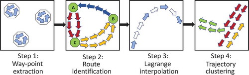
• In the route segmentation step, which is presented in Section 3.2, the compete trajectories are represented as sequences of sub-trajectories, each one connecting a pair of intermediate waypoints, in the path from the origin to the destination port waypoints.

• In the Lagrange interpolation step, trajectories that are incomplete are reconstructed using polynomial interpolation. Section 3.3 provides a detailed description.

• The (sub-)trajectory clustering step introduces a variation of the DB-Scan algorithm that examines spatial, speed, and direction distances (or differences) in order to identify neighboring points and thus groups together sub-trajectories that are located at a close distance and have similar speeds and directions. The methodology followed in this step is explained in detail in Section 3.4.

The resulting maritime traffic model contains waypoints (vertices) that group the stop or turn points of multiple vessels and sub-trajectory clusters (edges) that contain statistics extracted from all vessels that sailed from one waypoint to another. Edge statistics represent the preferred ways of sailing between two waypoints. This output can be used for many use cases in the field of anomaly detection.

3.1. Waypoint extraction

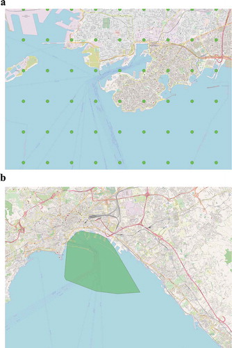
The first step of the approach identifies areas in which the vessels remain stationary (waypoints) for a reasonable amount of time. These waypoints can be either ports, anchorages or off-shore platforms, and will be used later in the route identification step. To this end, from the historical records we only keep the AIS positions which report zero speed and apply a spatial density-based clustering algorithm on them. In order to further reduce the amount of the data to be clustered and speed up the clustering process that follows, we apply a simple compression technique, in which the surveillance area is segmented into small tiles of 0.01 degrees of longitude and latitude (approximately $1k{m}^2$). Then, we further compress the dataset and keep only the temporally first position of each vessel per tile. The idea behind this simple compression step is that stationary vessels keep transmitting (almost) the same AIS position, thus adding no significant information for the steps that follow. Due to the fact that vessels can remain stationary for large periods of time, the amount of positions that are filtered out is significant (the percentage of positions that can be discarded can reach up to $99\mathrm{\%}$). The tile size selection was based on the dimensions of larger vessels such as Cargo, Tanker, or Passenger, which can reach up to $500$ meters in length. The tile size needs to be as small as possible, but not small enough to discard more positions from such larger vessels. Therefore, we selected the width and length of the tiles to be twice the size of the vessels ($1km$ of length and width). Figure 2(a) illustrates the tiles in which the surveillance area is segmented, while Figure 2(b) illustrates the resulting waypoint in the port of Napoli.

Figure 2. The waypoint extraction process

When the compression step is complete, the DB-Scan algorithm is used to group the remaining positions together into clusters. DB-Scan takes two parameters, eps (or epsilon), which specifies how close two points must be to be considered neighbors, and minPts, which specifies the number of neighbors a point must have to be included in a cluster. The parameters used in the algorithm are $eps=2km$ (an average radius for small or larger ports) and $minPts=10$ (minimum number of neighbouring vessel positions in a radius). In real-world terms, the aforementioned values means that we are seeking for regions, where the density is at least 10 vessels in a $12.5k{m}^2$ area, which is expected to detect rather dense clusters.

In the absence of port geometries, this waypoint extraction methodology can be useful, since the detected clusters denote the areas where vessels are moored or anchored. In order to better represent these areas we find the convex hull (Graham and Yao 1983) of each cluster (i.e. the minimum bounding geometry that contains all the cluster points).

3.2. Route identification

The second step in the pattern extraction process is the route identification. This step is of utmost importance since patterns must be extracted per itinerary. Let $A$ be the starting waypoint of a vessel and $B$ be the destination waypoint of the same vessel. The path a vessel followed to go from point $A$ to point $B$ is defined as a route $R_{A\to B}$. Itinerary $I_{A\to B}$ is defined as the sum of all routes of all vessels from $A$ to $B$:

(1) $\sum _{n=1}^{n=paths}{R}_{A\to B}=I_{A\to B}$(1)

Several vessels may follow the same route in order to move from the starting to the destination point, thus an itinerary may consist of routes travelled from one or more vessels. Trajectory is defined as a list $P$ of temporally sorted points or positions $p$ of a vessel. In short, a trajectory contains all of the AIS positions during a vessel’s lifespan. Algorithm 1 describes the process of route identification per vessel in detail. Initially, the algorithm is given a trajectory and a set of waypoints $W$. The previous waypoint $W_p$ is set to $-1$ (line 2) since in the beginning no waypoints have been encountered. All points of a vessel’s trajectory are examined (line 6) against the previously detected waypoints, in order to split the trajectory into routes. The within function is responsible for finding the waypoint $W_{p_k}$ (if any) that contains the trajectory point $p_k$ (line 7). When a trajectory point is found $within$ a waypoint for the first time (line 8) a new route starts and runs inside the waypoint (i.e. a vessel begins its route within the port) (lines 9–13). All the continuous trajectory points that intersect with the same waypoint (lines 15) are added to the route. When the first trajectory point that is out of the waypoint is found, then a new route begins, which heads to the next waypoint (i.e. the vessel sails to the next waypoint) (lines 16–22). This waypoint can either be the destination point of the route or simply an intermediate waypoint (e.g. an off-shore platform, or an intermediate port).

The process continues until all points of the trajectory are examined and the output is a list of routes within or between waypoints. Trajectories without starting or destination waypoints are ignored in the following steps of the proposed methodology. ‘Empty’ starting points occur when the first position of the trajectory is not within a waypoint, in which case the initial waypoint is set to $-1$ (line 2), while ‘empty’ destination waypoints occur when the vessel exited the surveillance area and we have no knowledge of its intermediate trajectory.

Algorithm 1 Route identification algorithm

Input: List of trajectory points $P$, Set of waypoints $W$

Output: List of routes $L_s$

1: function RouteIdentification ($P[]$)

2: $W_p$ $\leftarrow$ $-1$

3: $N$ $\leftarrow$ $length(P)$

4: $S$ $\leftarrow$ $[]$

5: $L_s$ $\leftarrow$ $[]$

6: for $k\leftarrow 1$ to $N$ do

7: $W_{p_k}$ $\leftarrow$ $within(p_k,W)$

8: if $W_{p_k}\ne \mathrm{\varnothing }$ then

9: if $W_{p_k}\ne W_p$ then

10: $S.append(p_k)$

11: $L_s.append(S)$

12: $S$ $\leftarrow$ $[]$

13: $W_p$ $\leftarrow$ $W_{p_k}$

14: else

15: $S.append(p_k)$

16: else

17: $W_{p_k}\leftarrow -1$

18: if $W_{p_k}\ne W_p$ then

19: $S.append(p_k)$

20: $L_s.append(S)$

21: $S\leftarrow []$

22: $W_p$ $\leftarrow$ $-1$

23: else

24: $S.append(p_k)$

25: $L_s.append(S)$

26: return $L_s$

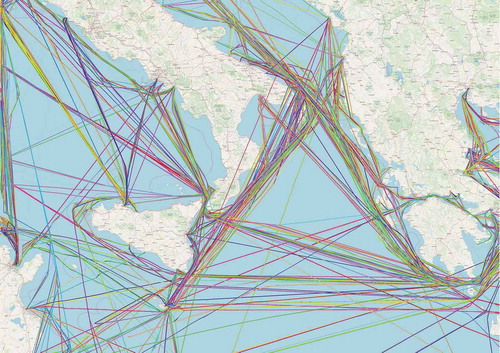
The output of the process is a set of lists of positions, each list representing a route. Several routes may refer to the same itinerary (Equation (1)(1) $\sum _{n=1}^{n=paths}{R}_{A\to B}=I_{A\to B}$(1) ). Figure 3 illustrates the output of the route identification step in the area between Italy and Greece. Each line depicted with different color represents a different route.

Figure 3. The output of the route identification step

3.3. Lagrange interpolation

The next step in the proposed workflow is the interpolation of the trajectories of every route. The reason behind this step is to fill the gaps that may arise in real vessel trajectories. Such gaps may affect the quality of the traffic patterns extracted with the proposed methodology, since they directly affect the quality of the clustering step that follows (see Section 3.4). It is quite common to have such gaps in vessel trajectories because although it is mandatory for vessels to carry an AIS transponder, it is not compulsory for the transponder to be switched on (Guerriero et al. (2008), Mazzarella et al. (2017), Kontopoulos et al. (2020)). This is a common tactic when vessels want to hide their tracks and conceal their whereabouts, in order to avoid piracy attacks, or perform an illegal act themselves (e.g. fishing in prohibited areas). Furthermore, AIS gaps in the trajectories may also happen, either due to bad weather conditions or because the receivers are deliberately jammed or, in rare occasions, because of packet collisions that take place when the AIS receivers are flooded with messages.

To tackle the problem of trajectory gaps, several studies have focused on finding an optimal interpolation algorithm for movement data only in recent years, either in the maritime domain (Hu et al. 2014, Sang et al. 2015, Nguyen et al. 2015, Du et al. 2017, Jie et al. 2017) or not (Long 2015). Nguyen et al. (2015) proposed a new method which includes linear interpolation and Cubic Hermit interpolation along with a mechanism to overcome problems of both approaches in order to fill in the gaps of missing AIS data. Hu et al. (2014) developed an interpolation model which is able to accurately estimate the vessel’s vectors of speed, heading and acceleration. Long (2015) proposed a new approach, called kinematic path interpolation, for interpolating movement data. A new interpolation technique is proposed in (Jie et al. 2017) and compared against Lagrange interpolation, Cubic spline interpolation and Hermite interpolation over AIS data, with all of the algorithms yielding an error between $0.072$ and $0.022$. In our work, we used the Lagrange interpolation (Berrut and Trefethen (1984), a well-known, established algorithm, that is preferred over Newton interpolation because it gives better approximations (Werner (1984). The interpolation itself is not the focus of our study, nevertheless, the various interpolation techniques can be used in the future to further study their effects in our approach. Given a set of $n$ data points

(2) $(x_0,y_0),\dots ,(x_j,y_j),\dots ,(x_{n-1},y_{n-1})$(2)

where no two $x_j$ are the same, the Lagrange interpolation is a linear combination

(3) $L(x)=\sum _{j=0}^{n-1}{y}_j\times l_j(x)$(3)

of Lagrange basis polynomials

(4) $l_j(x)=\prod _{m=0,m\ne j}^{n-1}\frac{x-x_m}{x_j-x_m}$(4)

where $0\le j<n$. In our case, $x$ and $y$ correspond to longitude and latitude respectively.

To apply Equation (3)(3) $L(x)=\sum _{j=0}^{n-1}{y}_j\times l_j(x)$(3) , we run a sliding window of $step=1$ and $size=3$ ($W_{1,3}=[p_0,p_1,p_2]$, where $p_j$ is a data point) in each trajectory, in order to always use $n=3$ data points¹ to create the polynomials ($2^{nd}$ degree polynomial). Since the Lagrange interpolation requires $O(n^2)$ multiplications and subtractions to evaluate the interpolation at a point, higher degree polynomials require more time to calculate. Furthermore, higher order polynomial interpolations suffer from the Runge’s phenomenon (Fornberg and Zuev 2007), which means that the generated curve tends to oscillate at the edges of an interval, resulting in erroneous interpolations. At each window $W_{1,3}$, a curve is generated by applying Equation (3)(3) $L(x)=\sum _{j=0}^{n-1}{y}_j\times l_j(x)$(3) on $W_{1,3}$. Next, we calculate the $x$-axis distance and the temporal distance between data points $p_1$ and $p_2$ such that:

(5) $D_x=p_{x_1}-p_{x_2}$(5)

and

(6) $D_t=p_{t_1}-p_{t_2}$(6)

In order to calculate the number of interpolating points to be added to the trajectory, we take into account the minimum transmission frequency of the AIS, which is $T_f=3$ minutes.² By dividing the temporal distance with $T_f$ we calculate the number of interpolating positions $k$ (Equation (7))(7) $k=\frac{D_t}{T_f}$(7) . Later, we divide the spatial distance with $k$ to calculate the spatial increment $x_{incr}$ (Equation (8)(8) $x_{incr}=\frac{D_x}{k}$(8) ), which indicates how much the vessel has moved in the $x$-axis at each time-frame of the missing trajectory.

(7) $k=\frac{D_t}{T_f}$(7)

(8) $x_{incr}=\frac{D_x}{k}$(8)

Since we know that every $3$ minutes the vessel moves by $x_{incr}$ and that the vessel has transmitted $k$ positions in total during the communication gap, it is easy to calculate the corresponding values ($y$, speed and heading) of the interpolating positions. Algorithm 2 describes the process of calculating the aforementioned values in detail.

Algorithm 2 Position interpolation per window $W_{1,3}$

Input: $p_1$,$k$, $T_f$, $x_{incr}$

Output: List of interpolating positions $L_p$

1: function PositionInterpolation($p_1$,$k$,$T_f$,$x_{incr}$)

2: $P_{previous}$ $\leftarrow$ $p_1$

3: $L_p$ $\leftarrow$ $[]$

4: for $i\leftarrow 1$ until $k$ do

5: $timestamp$ $\leftarrow$ $P_{previous}.timestamp+T_f$

6: $longitude$ $\leftarrow$ $P_{previous}.longitude+x_{incr}$)

7: $latitude$ $\leftarrow$ $lagrangeInterpolation(longitude)$

8: $distance$ $\leftarrow$ $haversineFormula(P_{previous},longitude,latitude)$

9: $speed$ $\leftarrow$ $distance/T_f$

10: $bearing$ $\leftarrow$ $calculateHeading(P_{previous},longitude,latitude)$

11: $L_p.append((timestamp,longitude,latitude,speed,bearing))$

12: $P_{previous}$ $\leftarrow$ $(timestamp,longitude,latitude,speed,bearing)$

13: return $L_p$

At each step of the iteration (line 4) the new interpolating timestamp and longitude is calculated by adding the corresponding increment values (lines 5 and 6 respectively), while the new latitude value is calculated using the Lagrange formula (line 7). To calculate the speed (line 9), we first need to calculate the distance between the previous and the current position (line 8). We use the Haversine formula because it takes into account the earth’s curvature. Then, the new heading is calculated by using simple trigonometric functions (line 10). Finally, the newly created interpolating position is added to the list (line 11) and becomes the previous position (line 12) as the iteration proceeds. To constrain the interpolation from creating unrealistic positions, we apply the interpolation to each route $R_{A\to B}$, after positions inside waypoints have been removed. Waypoints contain a large amount of positions that are anchored or moored, which means that positions will be scattered in a small area inside the waypoint, rather than follow a specific kinematic path, introducing extreme curvatures and extreme speed values. Moreover, routes that have a gap equal to or more than 24 hours are removed from the process.

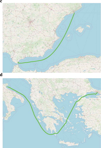
Figure 4 visualizes the result of the Lagrange interpolation applied to two distinct trajectories with large communication gaps. Figure 4(a,b) illustrate the trajectories with the communication gaps. Figure 4(a), shows a vessel that is traveling towards Barcelona, Spain, but the majority of its trajectory is missing. Similarly, Figure 4(b) visualizes a vessel that is traveling from the Ionian sea towards the Aegean sea, when a large communication gap appears at the south side of the Peloponnese. Figure 4(c,d) illustrate the same trajectories after the Lagrange interpolation. In both cases, our approach at interpolating missing positions manages to fill in the missing segments efficiently.

Figure 4. Examples of Lagrange interpolation applied to two trajectories

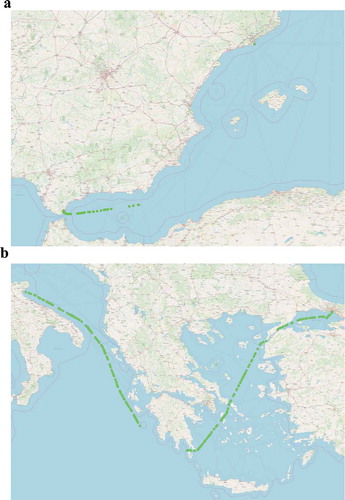
  Figure 4. Countinued

3.4. Trajectory clustering

The final step of the approach refers to the clustering of the trajectories that have the same itinerary $R_{A\to B}$. The typical algorithm for clustering the points of one or more trajectories is DB-Scan (Ester et al. (1996)), which is employed as a density-based spatial clustering method. Our proposed DB-Scan version uses 3 parameters to specify the proximity of candidate vessel AIS signals (positions):

• $s$: absolute difference of the speed between two positions (speed-based)

• $h$: absolute difference of the course-over-ground (CoG) between two positions (heading-based)

• $eps$: Haversine distance between two positions (spatial-based)

Therefore, for each position in a vessel’s trajectory we keep: i) the vessel’s speed, ii) the vessel’s direction (course over ground), and iii) its latitude and longitude coordinates. Then, three different thresholds are employed for deciding whether the positions from two different vessel trajectories are neighbors: the speed difference threshold $s$, the heading difference threshold $h$ and the distance threshold $eps$. When two positions from the same or different vessel trajectories have an absolute difference in all three dimensions that is below the threshold, the trajectory points are clustered together.

Figure 5 illustrates the differences between the two variants of the DB-Scan algorithm. Figure 5(a)³ on the left illustrates the original DB-Scan algorithm, that uses only the spatial distance as a neighboring criterion. Figure 5(b), on the right, depicts the modified DB-Scan for moving objects, which considers two (multi-dimensional) points (comprising position, direction and speed dimensions) to be close to each other (‘neighbors’ in DB-Scan notation) when the positions are spatially close to each other, and there are small differences in direction and speed.

Figure 5. Comparison of DB-Scan implementations

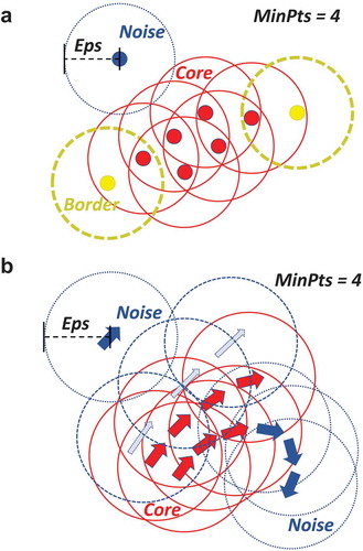
Each color in Figure 5(b) represents a different cluster. Red arrows belong to the same cluster because they are close to each other and have approximately the same speed and heading. Dashed thin blue arrows indicate a different cluster because they have a higher speed from the red arrows. Dotted thick blue arrows indicate outliers, which are either away, or have different speed or direction from all their neighbouring vectors. Specifically, dotted thick blue arrows at the bottom right have a different direction from the rest, while the dotted thick blue arrow at the top is away in terms of space.

Before applying the modified DB-Scan algorithm, we first segment the surveillance area into tiles of 0.2 degrees. The choice of this resolution of the grid was made because most of the weather services⁴ use the same resolution, thus integration with such services is easier, allowing us to further extend our approach in the future (e.g. enrich each tile with weather information to explain unexpected vessel movement behaviors). Furthermore, we do not need a tile size as small as the one mentioned in Section 3.1 because the small tile size is not ideal for the representation of the movement of multiple vessels (in small tile sizes significantly less number of vessels is located inside the same tile, especially in more sparse areas). On the other hand, the segmentation in larger tiles allows for better examination of multiple vessel behavior per area, since vessels in different areas might move in a different way. Then, we apply the clustering algorithm in each tile and for each itinerary $R_{A\to B}$ in each tile separately (each tile may contain more than one itinerary). The parameters of the DB-Scan are extracted from the data in each tile-itinerary pair. The $s$ parameter is the standard deviation of the speed between the positions of each pair. Similarly, $h$ and $eps$ is the standard deviation of heading and Haversine distance between the positions of each pair, respectively. We use the standard deviation because it measures the amount of variation or dispersion of a set of values. Positions with the lowest dispersion of speed, heading and distance need to be grouped together. $minPts$ is set to $6$ because we need at least two $3$-position-length routes per itinerary. $3$ is the minimum number of positions a trajectory should have to be considered valid. Therefore, clusters with one route are not considered common and are excluded from the process.

To have more accurate clustering results, we exclude positions that are located inside the waypoints. Since waypoints are areas of interest through which vessels frequently report zero speed, it can be easily inferred that the waypoints might be ports, platforms or anchorage areas. Furthermore, since waypoints are extracted from all the vessels frequently reporting zero speed, it is safe to assume that vessel behavior will be similar inside them.

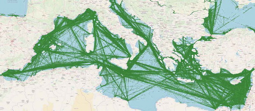
Finally, after the trajectory clustering process completes, the clusters are converted into convex hulls. The result is a set of convex hulls, each one annotated with the itinerary $R_{A\to B}$ it belongs to. Therefore, each itinerary can be represented as a set of convex hulls indicating the spatial boundaries the vessels must move in when following $R_{A\to B}$. Moreover, each convex hull contains statistics for the speed and heading such as minimum/maximum speed/heading, representing behavioral boundaries for the vessels. Any deviation from these spatial/behavioral boundaries is an anomaly which requires further attention and examination from the authorities. For a visual illustration of anomaly detection in maritime routes, consider Figure 6, which demonstrates examples of normal and abnormal or deviating behavior. The green semi-transparent polygons represent the convex hulls. The red circles indicate the positions of the vessel while the red lines simply connect these positions to illustrate the path followed. Figure 6(a) illustrates a vessel travelling towards Olbia city in Northern Sardinia which moves inside the spatial boundaries of the itinerary indicated by the convex hulls. It can also be seen that vessels that travel towards Olbia city follow two paths before entering the port. Figure 6(b) illustrates a vessel that departed from Barcelona, Spain which shortly after its departure, deviates from the spatial boundaries indicated by the convex hulls. These convex hulls can be used to evaluate in real-time, the moment an AIS position is received, whether the vessel deviates from the normal behavior or not. Figure 7 visualizes the output of the proposed methodology presented in Section 3 applied in all Cargo vessels sailing in the Mediterranean sea representing their ‘patterns-of-life’.

Figure 6. Examples of normal and anomalous behavior

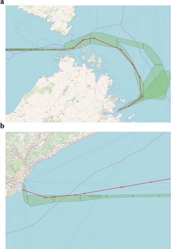
Figure 7. The output of the proposed methodology in the Mediterranean sea

4. Distributed architecture

The methodology described in the previous section requires the processing of a tremendous amount of historic AIS data. Moreover, the aforementioned algorithms described, such as the DB-Scan algorithm, perform CPU, and memory intensive operations. For that reason, the entire approach is implemented in a distributed fashion using the Apache Spark $\mathrm{2.4.4}$⁵ platform.

Apache Spark is a well-known, mature, and distributed MapReduce framework which allows the in-memory batch processing of Big Data. Due to its nature and its maturity in the field of Big Data and batch processing, it is often preferred over other frameworks such as Apache Hadoop,⁶ Apache Storm,⁷ Apache Flink⁸ when processing historic data. Apache Hadoop, similar to Spark, is a distributed framework that allows for the distributed processing of large data sets across clusters of computers. It is famous for the use of the MapReduce programming paradigm and the Hadoop Distributed File System (HDFS), which stores files in a Hadoop-native format and parallelizes them across a cluster. The main difference between these two frameworks is that Spark works in memory which results in a huge performance increase. Apache storm is a framework for real-time distributed computation of data. It can process unbounded streams of data and it is the equivalent of Hadoop for real-time processing. Apache Flink is a framework for in-memory distributed stateful computations over unbounded and bounded data streams. It can work well with both batch and stream processing due to its inherent ability to treat data as streams of events. Unfortunately, although Apache Flink is promising, it lacks the maturity of Apache Spark. Finally, it is worth noting Kafka streams⁹ which is a fast-emerging framework for building real-time applications and microservices. Taking into account all of the properties of these platforms, we chose Apache Spark for the implementation of our methodology because of its maturity in batch processing data.

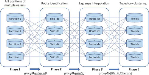
Figure 8 illustrates the distributed workflow of the proposed methodology. Initially, the historic AIS data are distributed over $n$ partitions with no partition strategy (Phase $1$). In order to extract the routes of each trajectory and run Algorithm 1 in parallel (Phase $2$), data are grouped by the ship id. Therefore, a partition contains all of the AIS data that refer to the same trajectory or ship id. In addition, a partition may contain one or more trajectories. After Phase $2$ is complete and each trajectory is segmented into sub-trajectories or routes, we need to apply the Lagrange interpolation on each route (Phase $3$). To this end, data are now grouped by the route id which allows for better re-balancing of data – trajectories are not segmented into an equal number of segments. Next, each AIS position is mapped to a spatial index or tile id. Each tile id may contain one or more itineraries, therefore, data are now grouped by pairs of tile id/itinerary in order to apply the modified DB-Scan algorithm to each pair (Phase $4$). This results in the processing of several thousands or several millions of DB-Scan algorithms in parallel. The number of DB-Scan algorithms depends on the number of tiles and the number of itineraries per tile. Finally, after the clusters are formed, each cluster is converted to a convex hull.

Figure 8. The distributed workflow of the proposed methodology

5. Experimental evaluation

This section describes the datasets used in the experiments as well as the performance of the proposed methodology. The experimental evaluation presented below was performed on a cluster consisting of 4 machines with 4 cores (Intel(R) Xeon(R) CPU E5-2650 0 @ 2.00 GHz) and 8 GB of RAM each, totalling in 16 cores and 32 GB of RAM, running Ubuntu 18.04 LTS with Java OpenJDK 1.8, Scala 2.11.8 and Apache Spark 2.4.4.

5.1. Dataset description

The dataset that was used was provided by MarineTraffic¹⁰ and contains in total $35,042,110$ AIS messages from $9,335$ vessels sailing in the Mediterranean during a three-month period (May 2016 to July 2016). The total size of the dataset is, originally, $4.4$ GB. To evaluate our proposed methodology, we separated the dataset into three vessel types, namely Cargo, Tanker, and Passenger. These types of vessels typically follow predefined shipping lanes between two ports or waypoints, making them suitable for the evaluation of our approach. For each vessel type and for each unique vessel identifier per type, routes were extracted as described in Section 3.2 and Lagrange interpolation was used in the routes as described in Section 3.3. The resulting dataset was comprised of $861,093$ itineraries and $332,645,827$ AIS positions, totalling in $59$ GB. Table 1 shows the size of the dataset and the number of AIS positions per vessel type, while Table 2 shows the number of itineraries and the number of vessels per vessel type. In Table 1, the first two columns after the vessel type indicate the size of the dataset before the interpolation, while the next two columns indicate the size of the dataset after the interpolation was performed. To the best of our knowledge, this is the first time in the literature that a dataset of this magnitude of maritime data has been used to evaluate similar traffic models.

Table 1. Dataset size

Vessel Type	# Positions	Size	# Interpolated positions	Size
Cargo	21,049,968	2.7 GB	181,392,045	32 GB
Tanker	6,762,563	888 MB	68,028,555	12 GB
Passenger	7,229,579	974 MB	83,225,227	15 GB

Table 2. Dataset characteristics

Vessel Type	# itineraries	# vessels
Cargo	388,059	6,089
Tanker	117,473	2,027
Passenger	355,561	1,219

5.2. Experimental results

The evaluation of the proposed methodology is two-fold. First, we need to evaluate the model on how successful it is at representing the maritime traffic patterns. Second, we need to evaluate the compactness of the resulting convex hulls representing the movement of the vessels. To test the former, we used 10-fold cross-validation on the itineraries of each of the three datasets containing different vessel types, as shown in Table 2, thus always maintaining a training-test split of $90\mathrm{\%}-10\mathrm{\%}$, respectively. On each fold, $90\mathrm{\%}$ of the itineraries were used to perform the Lagrange interpolation, the modified DB-Scan algorithm and create the convex hulls, while the rest of the itineraries were used to measure the accuracy of the convex hulls. Since each DB-Scan algorithm is performed on each tile, this results in running several thousands of DB-Scan algorithms in parallel (see Section 4). In our case, performance is measured as in (Pallotta et al. 2013) and (Coscia et al. 2018) as the percentage of AIS positions of the test set that fall within the convex hulls and use the term ‘accuracy’ to refer to it. Specifically:

(9) $Accuracy=\frac{\mathrm{\#}ofAISpositionswithintheconvexhulls}{\mathrm{\#}oftotalAISpositions}$(9)

Table 3 shows the averaged accuracy achieved by our methodology for each vessel type. The results show that our approach can model, in the best case, up to $98.56\mathrm{\%}$ of the maritime traffic of the Cargo vessels. Passenger vessels achieve the lowest performance of $94.4\mathrm{\%}$ and Tanker vessels lie in the middle ($94.62\mathrm{\%}$). This can be explained since the number of itineraries and the number of Cargo vessels is greater compared to the other two vessel types, yielding a better representation of the maritime traffic.

Table 3. 10-fold cross validation results

Vessel Type	Accuracy (%)
Cargo	98.56
Tanker	94.62
Passenger	94.4

To further test our approach, this time, we used as a training set the first two months of the dataset (May and June) and tested the accuracy on the remaining month (July). Similar to the 10-fold cross-validation experiment, we used the training set to perform the Lagrange Interpolation, the modified DB-Scan algorithm, and create the convex hulls, while the test set was used to measure the accuracy (Equation (9))(9) $Accuracy=\frac{\mathrm{\#}ofAISpositionswithintheconvexhulls}{\mathrm{\#}oftotalAISpositions}$(9) . Table 4 shows the achieved accuracy per vessel type.

Table 4. Accuracy results on the third month (July)

Vessel Type	Accuracy (%)
Cargo	97.65
Tanker	90.97
Passenger	97.95

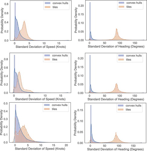
To evaluate the compactness of the convex hulls we compared our methodology with a baseline approach that instead of using clusters and convex hulls, it only uses the statistics extracted per tile of the surveillance area. To show that the statistics of the convex hulls are more representative of the vessel movement and more compact, we measured the standard deviation of the speed and heading of the AIS positions they contain. Similarly, we measured the standard deviation of the same features of the AIS positions contained in each tile. We note that there may be more than one convex hull per tile. Figure 9 illustrates the distribution plots of the standard deviation of speed and heading for each vessel type. Figures 9(a,c,e) illustrate the distribution plot of the standard deviation of speed, while Figures 9(b,d,f) illustrate the distribution plot of the standard deviation of heading. The blue line demonstrates the distribution of the convex hulls and the orange dashed line demonstrates the distribution of the tiles. We can observe that the standard deviations of the convex hulls are gathered to the left which indicate that we have lower values for the deviations. On the other hand, the standard deviations of the tiles tend to be in the middle of the Figures, which indicate larger values of standard deviations. From Figure 9 we can infer that the convex hulls are more compact and that the AIS positions located inside them have similar speed and heading.

Figure 9. Distribution plots for speed and heading of each vessel type

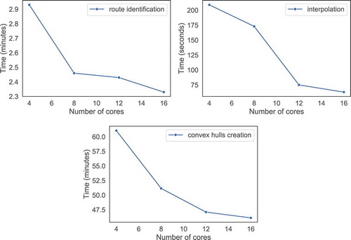
Finally, to demonstrate the scalability of the solution, we run for each step of the approach (route identification, interpolation, convex hulls creation), four experiments, each one with a different number of processing cores. To this end, due to the volume of the dataset and the time required for the entire methodology to extract the final set of convex hulls, we chose the vessel type with the least number of AIS positions, the Tanker vessels. Furthermore, we run the experiments in the first month of the dataset (May) and only in $10\mathrm{\%}$ of the vessels of the month, thus significantly reducing the size of the dataset. Consequently, we measured the time required for each experiment to be completed and illustrated the results in Figure 10. Figure 10(a) illustrates the time required for the route identification step to be executed using 4, 8, 12 and 16 processing cores. Similarly, Figure 10(b,c) illustrate the time required for the interpolation and the convex hulls creation steps to be completed, respectively. In each step, we can see that as the number of processing cores increases, the execution time of each step decreases, demonstrating that the proposed methodology can take advantage of multiple number of CPUs in a cluster to improve the execution time.

Figure 10. The scalability of the approach in each step

6. Discussion

As explained in Section 2 the proposed network abstraction model provides a compact way for representing repeating trajectories, such as the routes followed by cargo or passenger vessels. For this purpose, it performs a simplification of the route that relies on the main waypoints and the edges connecting them, making it comparable to other abstraction models. Compared to Arguedas et al. (2017), our methodology scales in much larger AIS datasets as shown in Section 5 (the Mediterranean sea, an area of $2.5\times 10^{6}k{m}^2$ compared to the Baltic sea, a much smaller surveillance area of $404.354k{m}^2$). Moreover, Arguedas et al. (2017) rely on several user-defined parameters and thresholds, which makes the fine-tuning of the maritime network more difficult.

As far as it concerns anomaly detection the proposed framework relies on the extracted network abstraction model for defining normal behaviours. In order to detect deviations, it is important for the extracted abstraction model to cover, as much as possible, the normal vessel route positions. The performance of the proposed model is at similar level to that of TREAD (Pallotta et al. 2013) in terms of AIS positions that fall within the extracted model against the total AIS positions. TREAD highly depends on the traffic density, thus managed to capture $95\mathrm{\%}$ of the total traffic in small high-density regions (e.g. the strait of Gibraltar) and much smaller percentages in regions with sparse vessel traces (e.g. 75% in the North Adriatic Sea and $40\mathrm{\%}$ in the Indian ocean). Our proposed methodology is able to capture $95\mathrm{\%}$ of the total maritime traffic in either dense or sparse regions of sea, due to the Lagrange interpolation that we perform on trajectories. Similarly, the proposed methodology of Coscia et al. (2018), which creates a graph-based representation, achieves a performance of $76.1\mathrm{\%}$ in the Atlantic Ocean off the coasts of Spain, France and in the English Channel.

7. Conclusion and next steps

In this work, we presented a distributed framework that captures the vessels’ behavior and extracts the patterns of their movement. Specifically, the findings of the proposed approach can be summarized in two major points: i) the resulting convex hulls manage to accurately represent the spatial boundaries of the vessel movement indicating that any future AIS position can be effectively predicted and placed in a certain geographic region ii) the convex hulls can effectively represent the behavior of the vessel movement in terms of speed and heading and detect possible anomalies and deviations. Although many early alerts and false alarms may arise, using the richer pattern information (direction and speed and position) as well as windowed averages of the latest vessel status it can be easier to distinguish true from false alarms (Kontopoulos et al. 2019). It is among our future steps to further examine this problem.

One interesting perspective that is to be studied further regarding the maritime traffic patterns is the experimental evaluation in large sparse geographic areas such as the Atlantic and the Pacific ocean. The resulting convex hulls in such sparse areas tend to be smaller compared to the convex hulls in dense areas such as ports due to the strict movement the vessels follow and the long linear trajectories.

Our next steps include the expansion of the network with more node types, such as turn-points that may represent capes, or areas of slow speed, such as canals. The integration of the framework with weather services that can provide added value to the definition of convex hulls and edges is also among the future steps. Finally, we are working on the use of the extracted maritime traffic patterns as a basis for a real-time anomaly detection and route monitoring system.

Acknowledgments

This work was supported by the MASTER and SmartShip Projects through the European Union’s Horizon 2020 research and innovation programme under the Marie-Slodowska Curie grant agreement no 777695 and 823916 respectively. The work reflects only the authors’ view and that the EU Agency is not responsible for any use that may be made of the information it contains.

Disclosure statement

No potential conflict of interest was reported by the author(s).

Data and codes availability statement

The code that supports the findings of this study is available in https://github.com/kontopoulos/ROUTER. The data cannot be made publicly available to protect research participant privacy and consent.

Supplementary material

Supplemental data for this article ccan be accessed here.

Additional information

Funding

This work was supported by the SmartShip [823916]; MASTER [777695].

Notes on contributors

Ioannis Kontopoulos

Ioannis Kontopoulos is currently a Ph.D. candidate at the Department of Informatics and Telematics of Harokopio University of Athens and works as a Research Associate at both the university and MarineTraffic. He received his BSc from the same department. The topic of his Ph.D. thesis is “Distributed Complex Event Recognition and Forecasting”. His main research interests include distributed and real-time processing, Big data analysis, high-performance computing (HPC), trajectory, and spatiotemporal analysis. He has participated in three EU funded projects such as DATACRON (H2020), MASTER (H2020), and Smartship (H2020).

Iraklis Varlamis

Iraklis Varlamis is an Associated Professor at the Department of Informatics and Telematics of the Harokopio University of Athens. He holds a Ph.D. in Informatics from Athens University of Economics and Business, Greece, and an MSc in Information Systems Engineering from UMIST, UK. He has been involved as a technical coordinator in a number of EU funded projects concerning knowledge management, data mining, machine learning, and expert systems. He has also coordinated several national R&D projects concerning data management and personalized delivery of information. He has authored more than 120 articles concerning text and graph mining and intelligent applications in social networks and the web and received more than 1800 citations. He has worked as a scientific coordinator or principal investigator in several collaborative research projects funded by National, EU (e.g. H2020 TEACHING, SustAGE, MASTER, FP7-Fortissimo) and International Funds (e.g. Qatar Funding-EM3).

Konstantinos Tserpes

Konstantinos Tserpes is an Assistant Professor at the Department of Informatics and Telematics of the Harokopio University of Athens. He holds a Ph.D. in the area of Distributed Systems from the school of Electrical and Computer Engineering of the National Technical University of Athens (2008). His research interests revolve around distributed systems, software and service engineering, Big Data analytics, and social systems. He has been involved in several EU and National funded projects leading research for solving issues related to scalability, interoperability, fault tolerance, and extensibility in application domains such as multimedia, e-governance, post-production, finance, e-health, and others. He has served as the scientific or general coordinator in several ICT projects such as +Spaces, SocIoS, Consensus, Fortissimo (FP7), and BASMATI (H2020) and the principal investigator for the projects ACCORDION, TEACHING, COLLABS, MASTER and SmartShip (H2020).

Notes

1. The minimum number of data points required to create a curve.

2. The transmission frequency of the AIS depends on the speed and the rate of change in course. The higher the values, the higher the transmission frequency. The highest transmission frequency is one position every $2$ seconds.

3. https://en.wikipedia.org/wiki/DBSCAN

4. https://www.noaa.gov/weather

5. https://spark.apache.org/

6. https://hadoop.apache.org/

7. https://storm.apache.org/

8. https://flink.apache.org/

9. https://kafka.apache.org/documentation/streams/

10. https://www.marinetraffic.com/

References

- Andrienko, N. and Andrienko, G., 2011. Spatial generalization and aggregation of massive movement data. IEEE Transactions on Visualization and Computer Graphics, 17, 205–219.
- Andrienko, N. and Andrienko, G., 2013. Visual analytics of movement: an overview of methods, tools, and procedures. Information Visualization, 12 (1), 3–24. doi:10.1177/1473871612457601
- Arguedas, V.F., Pallotta, G., and Vespe, M., 2017. Maritime traffic networks: from historical positioning data to unsupervised maritime traffic monitoring. IEEE Transactions on Intelligent Transportation Systems, 19 (3), 722–732. doi:10.1109/TITS.2017.2699635
- Berrut, J.P. and Trefethen, L.N., 1984. Barycentric Lagrange interpolation. Society for Industrial and Applied Mathematics, 46 (3), 501–517.
- Chatzikokolakis, K., et al., 2018. Mining vessel trajectory data for patterns of search and rescue. In: Proceedings of the Workshops of the EDBT/ICDT 2018 Joint Conference (EDBT/ICDT 2018), 26 March. Vienna, Austria, 117–124.
- Chen, J. and Meng, X., 2010. Clustering analysis of moving objects. In: Moving Objects Management, Chapter 11, 151–171. Springer.
- Coscia, P., et al. 2018. Multiple ornstein–uhlenbeck processes for maritime traffic graph representation. IEEE Transactions on Aerospace and Electronic Systems, 54 (5), 2158–2170. doi:10.1109/TAES.2018.2808098.
- Du, H., et al., 2017. An algorithm for vessel’s missing trajectory restoration based on polynomial interpolation. In: 4th international conference on transportation information and safety, ICTIS 2017. Edmonton, Canada, 825–830.
- Ester, M., et al., 1996. A density-based algorithm for discovering clusters a density- based algorithm for discovering clusters in large spatial databases with noise. In: Proceedings of the second international conference on knowledge discovery and data mining, KDD’96. Portland: Oregon AAAI Press, 226–231.
- Etemad, M., et al., 2019. A trajectory segmentation algorithm based on interpolation- based change detection strategies. In: Workshop Proceedings of the EDBT/ICDT 2019 Joint Conference, Vol. 2322. Lisbon, Portugal: CEUR.
- Etemad, M., Júnior, A.S., and Matwin, S., 2018. Predicting transportation modes of GPS trajectories using feature engineering and noise removal. In: 31st Canadian conference on artificial intelligence. Toronto, ON, 259–264.
- Fornberg, B. and Zuev, J., 2007. The Runge phenomenon and spatially variable shape parameters in RBF interpolation. Computers and Mathematics with Applications, 54 (3), 379–398. doi:10.1016/j.camwa.2007.01.028
- Fu, Z., Hu, W., and Tan, T., 2005. Similarity based vehicle trajectory clustering and anomaly detection. In: IEEE international conference on image processing, ICIP 2005, Vol. 2. Genoa, Italy, II–602.
- Graham, R.L. and Yao, F.F., 1983. Finding the convex hull of a simple polygon. Journal of Algorithms, 4 (4), 324–331. doi:10.1016/0196-6774(83)90013-5
- Guerriero, M., et al., 2008. Radar/AIS data fusion and SAR tasking for maritime surveillance. In: 11th international conference on information fusion. Cologne, Germany, 1–5.
- Hexeberg, S., et al., 2017. AIS-based vessel trajectory prediction. In: 20th international conference on information fusion, FUSION 2017. Xi’an, China, 1–8.
- Holst, A., et al., 2012. A joint statistical and symbolic anomaly detection system: increasing performance in maritime surveillance. In: 15th international conference on information fusion, FUSION 2012. Singapore, 1919–1926.
- Holst, A. and Ekman, J., 2003. Anomaly detection in vessel motion. Internal Report Saab Systems, Järfälla, 4.
- Hu, Q., et al., 2014. An algorithm for interpolating ship motion vectors. TransNav, the International Journal on Marine Navigation and Safety of Sea Transportation, 8, 35–40. doi:10.12716/1001.08.01.04.
- Jie, X., et al., 2017. A novel estimation algorithm for interpolating ship motion. In: 4th international conference on transportation information and safety, ICTIS 2017. Banff, Alberta, Canada, 557–562.
- Kontopoulos, I., et al., 2020. Real-time maritime anomaly detection: detecting intentional AIS switch-off. International Journal of Big Data Intelligence. doi:10.1504/IJBDI.2020.107375.
- Kontopoulos, I., Varlamis, I., and Tserpes, K., 2019. Uncovering hidden concepts from AIS data: A network abstraction of maritime traffic for anomaly detection. In: “Multiple-aspect analysis of semantic trajectories” workshop of the ECML/PKDD 2019 joint conference. Wurzburg, Germany: Springer, 6–20.
- Laxhammar, R., 2008. Anomaly detection for sea surveillance. In: 11th international conference on information fusion, FUSION 2008. Cologne, Germany, 1–8.
- Laxhammar, R., Falkman, G., and Sviestins, E., 2009. Anomaly detection in sea traffic- a comparison of the Gaussian mixture model and the Kernel density estimator. In: 12th international conference on information fusion, FUSION 2009. Seattle, Washington, 756–763.
- Le Guillarme, N. and Lerouvreur, X., 2013. Unsupervised extraction of knowledge from S-AIS data for maritime situational awareness. In: 16th international conference on information fusion, FUSION 2013. Istanbul, Turkey, 2025–2032.
- Lee, J.G., Han, J., and Whang, K.Y., 2007. Trajectory clustering: a partition-and-group framework. In: ACM SIGMOD international conference on management of data, SIGMOD/PODS 2007. Beijing, China, 593–604.
- Li, Y., Han, J., and Yang, J., 2004. Clustering moving objects. In: 10th ACM SIGKDD international conference on knowledge discovery and data mining, KDD 2004. Seattle, WA, 617–622.
- Liu, B., et al., 2014. Knowledge-based clustering of ship trajectories using density-based approach. In: IEEE international conference on big data, big data 2014. Washington DC, 603–608.
- Liu, W., Wang, Z., and Feng, J., 2008. Continuous clustering of moving objects in spatial networks. In: I. Lovrek, R.J. Howlett, and L.C. Jain, ed. Knowledge-based intelligent information and engineering systems. Berlin, Heidelberg: Springer Berlin Heidelberg, 543–550.
- Long, J., 2015. Kinematic interpolation of movement data. International Journal of Geographical Information Science, 30, 1–15.
- Mazzarella, F., et al., 2017. A novel anomaly detection approach to identify intentional AIS on-off switching. Expert Systems with Applications, 78, 110–123. doi:10.1016/j.eswa.2017.02.011.
- Montewka, J., Kujala, P., and Ylitalo, J., 2009. The quantitative assessment of marine traffic safety in the Gulf of Finland, on the basis of AIS data. Proceedings of the 14th international scientific and technical conference on marine traffic engineering. Malmö, Sweden, 105–115.
- Nguyen, V., Im, N.K., and Lee, S.M., 2015. The interpolation method for the missing AIS data of ship. Journal of Navigation and Port Research, 39, 377–384. doi:10.5394/KINPR.2015.39.5.377
- Ossama, O., Mokhtar, H.M., and El-Sharkawi, M.E., 2011. An extended k-means technique for clustering moving objects. Egyptian Informatics Journal, 12 (1), 45–51. doi:10.1016/j.eij.2011.02.007
- Pallotta, G., Vespe, M., and Bryan, K., 2013. Vessel pattern knowledge discovery from AIS data: A framework for anomaly detection and route prediction. Entropy, 15 (6), 2218–2245. doi:10.3390/e15062218
- Sang, L.Z., et al., 2015. A novel method for restoring the trajectory of the inland waterway ship by using AIS data. Ocean Engineering, 110, 183–194. doi:10.1016/j.oceaneng.2015.10.021.
- Stefanakis, E., 2017. mR-V: line simplification through mnemonic rasterization. Geomatica, 70 (4), 269–282.
- Tampakis, P., et al., 2018. Time-aware sub-trajectory clustering in Hermes@ PostgreSQL. In: 2018 IEEE 34th international conference on data engineering (ICDE). Paris, France, 1581–1584.
- Varlamis, I., et al., 2019. A network abstraction of multi-vessel trajectory data for detecting anomalies. In: Workshop proceedings of the EDBT/ICDT 2019 joint conference, Vol. 2322. Lisbon: Portugal CEUR.
- Varlamis, I., Tserpes, K., and Sardianos, C., 2018. Detecting search and rescue missions from AIS data. In: IEEE 34th international conference on data engineering workshops, ICDEW 2018. Paris, France, 60–65.
- Werner, W., 1984. Polynomial interpolation: Lagrange versus Newton. Mathematics of Computation, 43 (167), 205–217. doi:10.1090/S0025-5718-1984-0744931-0
- Yap, P., 2002. Grid-based path-finding. In: Proceedings of the 15th conference of the Canadian society for computational studies of intelligence on advances in artificial intelligence, AI ’02. London, UK: Springer-Verlag, 44–55.