A comparative study of heterogeneous ensemble-learning techniques for landslide susceptibility mapping

ABSTRACT

This study introduces four heterogeneous ensemble-learning techniques, that is, stacking, blending, simple averaging, and weighted averaging, to predict landslide susceptibility in Yanshan County, China. These techniques combine several state-of-the-art classifiers of convolutional neural network, recurrent neural network, support vector machine, and logistic regression in specific ways to produce reliable results and avoid problems with the model selection. The study consists of three main steps. The first step establishes a spatial database consisting of 16 landslide conditioning factors and 380 historical landslide locations. The second step randomly selects training (70% of the total) and test (30%) datasets out of grid cells corresponding to landslide and non-slide locations in the study area. The final step constructs the proposed heterogeneous ensemble-learning methods for landslide susceptibility mapping. The proposed ensemble-learning methods show higher prediction accuracy than the individual classifiers mentioned above based on statistical measures. The blending ensemble-learning method achieves the highest overall accuracy of 80.70% compared to the other ensemble-learning methods.

KEYWORDS:

• Landslide susceptibility mapping
• heterogeneous ensemble
• stacking
• blending
• deep neural networks

1. Introduction

Landslides are destructive natural disasters that pose a serious threat to human life and property (Mandal and Mandal 2018). According to the Emergency Events Database,¹ landslides worldwide have caused 66,438 deaths and economic loss of approximately 10.8 billion U.S. dollars from 1900 to 2020 (Guha-Sapir et al. 2020). Landslide susceptibility refers to the possibility of a landslide occurring in a certain area based on a series of geological environmental conditions (Guzzetti et al. 2006). An important step for mitigation and prevention is to produce accurate landslide susceptibility maps in landslide-prone areas.

In the past few decades, studies have developed various methods for landslide susceptibility mapping (LSM), which can be classified as qualitative and quantitative methods (Guzzetti et al. 1999). Qualitative methods rely upon expert knowledge to characterize landslide susceptible zones, such as the analysis of landslide inventory (Galli et al. 2008), analytic hierarchy process (Yalcin 2008, Pourghasemi et al. 2012), and weighted linear combination (Ayalew et al. 2004, Akgun et al. 2008). Quantitative methods include deterministic methods and statistical methods. Deterministic methods are static and apply physical laws to identify slope instability (Anagnostopoulos et al. 2015, Alvioli and Baum 2016), while statistical methods are based on functional expressions between inferred contributing factors and landslide occurrence, such as logistic regression (LR) (Ayalew and Yamagishi 2005, Lee and Pradhan 2007, Wang et al. 2017, Lombardo and Mai 2018), multi-criteria decision analysis (Feizizadeh and Blaschke 2013, Kavzoglu et al. 2014, Erener et al. 2016), bivariate statistical analysis (Yalcin 2008, Althuwaynee et al. 2014), and machine learning methods (Shahri et al. 2019, Wang et al. 2019a, Pham et al. 2019b). Recent studies use meta-heuristic optimization algorithms to tune model parameters for better performance (Termeh et al. 2018, Chen et al. 2019, Wang et al. 2019c). For example, grey wolf and biogeography-based optimization algorithms optimize the parameters of adaptive neuro-fuzzy inference system for LSM (Jaafari et al. 2019). Other optimizers include the genetic algorithm, differential evolution, and particle swarm optimization (Chen et al. 2017).

Deep learning techniques outperform the other machine learning methods in the fields of natural language processing, object detection, and scene classification (Collobert and Weston 2008, Li et al. 2010, Han et al. 2018) and have shown success in spatial prediction of landslides. Successful examples include sparse autoencoders (Huang et al. 2019), convolutional neural network (CNN) (Sameen et al. 2019, Hajimoradlou 2019, Ullo et al. 2019, Wang et al. 2019b, Fang et al. 2020), recurrent neural network (RNN) (Mutlu et al. 2019, Wang et al. 2020b) and residual networks (Sameen and Pradhan 2019).

However, these successful examples have some shortcomings that limit the prediction performance of individual algorithms. For example, training data for LSM are often limited, and individual learning algorithms may miss the best-fit function or the true distribution of the sample set from the hypothesis space (Dietterich 1997, Wang et al. 2011, Korzh et al. 2017). Researchers hence develop ensemble-learning techniques for LSM to improve the prediction accuracy of a single classifier, such as Adaboost (Bui et al. 2016, Pham et al. 2017), Bagging (Bui et al. 2016, Truong et al. 2018), random subspace (Shirzadi et al. 2017, Pham et al. 2019b), and rotation forest (Hong et al. 2018, Pham et al. 2019a). These ensemble-learning techniques are homogeneous because they combine the same classifier multiple times to construct an aggregated model. As such, the shortcomings of a single classifier may multiply, which is undesirable for the result. Meanwhile, the study areas vary geographically in landslide susceptibility prediction. Different areas have different geo-environmental conditions, and homogeneous ensemble-learning techniques for LSM dismiss the geographic variabilities in an area.

Heterogeneous ensemble-learning techniques that integrate different single classifiers have shown strong nonlinear representation in many fields (Sesmero et al. 2015, Lee et al. 2019a, Wang et al. 2019d). Heterogeneous ensemble-learning can capture the advantages of different landslide prediction models and are therefore more robust and generalizable than homogeneous ensemble-learning. Moreover, the difficulty of model selection for LSM can be avoided to some extent, as heterogeneous ensemble-learning techniques can maintain heterogeneity by integrating any types of base classifier. Nevertheless, the application of heterogeneous ensemble-learning techniques in LSM is still scarce in the literature. To fill the knowledge gap in LSM, we evaluated four heterogeneous ensemble-learning techniques, stacking, blending, simple averaging (SA), and weighted averaging (WA), to predict landslide susceptibility in Yanshan County, China. These techniques combine several state-of-the-art classifiers of CNN, RNN, support vector machine (SVM), and LR in specific ways to produce reliable results and avoid problems with model selections. Our study makes the following three LSM innovations. (1) We used four heterogeneous ensemble-learning techniques for LSM by combining deep learning methods and conventional machine learning methods. Specifically, we chose CNN and RNN deep learning methods for their performance over other conventional methods (Xiao et al. 2018, Ullo et al. 2019, Sameen et al. 2019, Wang et al. 2019b), SVM machine learning model for its strong predictability and generalizability (Pradhan 2013, Yu et al. 2016, Kumar et al. 2017), and LR statistical method for its common applications (Reichenbach et al. 2018). (2) We explored the ensembled deep learning techniques in LSM. The CNN and RNN have been previously used to predict landslides, but only as single prediction models (Wang et al. 2019b; 2020b). Unlike in previous studies, in this study, we used deep learning techniques as part of the proposed heterogeneous framework. (3) This study provides the details of heterogeneous ensemble-learning methods and outcome assessment. Our literature review shows that heterogeneous ensemble-learning is still rarely used in LSM, and many studies only used the simple heterogeneous ensemble-learning techniques, such as SA and WA. In this study, we applied the above simple heterogeneous methods and two meta heterogeneous methods of stacking and blending for LSM. We validated the effectiveness of the proposed ensemble-learning methods with several statistical measures.

2. Study area and data

2.1. Study area

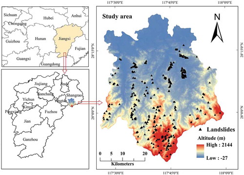
Yanshan County is located in the northeastern Jiangxi Province, China, covering an area of approximately 2178 km². The elevation of the study area ranges from −27 m to 2,144 m above sea level (Figure 1). The south of Yanshan County is a middle-low mountainous area with dense forests and hilly land with plenty of cultivated land, and the north of the county is covered with valleys and plains. The terrain of the study area gradually slopes from southeast to northwest, and can be divided into three geomorphic subdivisions. The first geomorphic subdivision is a middle-low mountainous area in the southern part of the study area, with an altitude between 500 m and 2100 m. This subdivision area has steep terrain with overlapped mountains, and the valley is eroded and cut into a V shape. The geomorphic area is mainly composed of granite, pyroclastic rock, and eruptive rock. The second geomorphic subdivision is located in the central area of Yanshan County. The elevation of this subdivision ranges from 100 m to 500 m, and the eroded valley is V- and U-shaped. The area is mainly composed of Sinian and Qingbaikou metamorphic rocks, Triassic and Jurassic clastic rocks, Carboniferous and Permian carbonate rocks, and Yanshanian magmatic rocks. The third geomorphic subdivision is located in the northern part of the study area, mainly distributed in low hills and valley plains. Red sandstone and glutenite are the main lithology in this area.

Vegetation in the study area is very rich, with a forest coverage rate of 73.67%. There are five main plant types in the area, including subtropical evergreen coniferous forest, coniferous and broad-leaved mixed forest, evergreen broad-leaved forest, subtropical coniferous forest, and bamboo forest. Yanshan County has a subtropical humid climate and is affected by the Pacific and Indian Ocean monsoons. According to the Jiangxi Provincial Meteorological Bureau,² the average annual rainfall from 1959 to 2007 was 1700‒2100 mm. Moreover, landslides are the most extensive and harmful geological disasters in Yanshan County, accounting for 50.4% of the total number of disaster events.

Figure 1. Location of the study area

2.2. Landslide inventory mapping

The existing landslide database demonstrates the spatial characteristics of landslide events in a given area, which helps to understand the relationship between the conditioning factors and landslide occurrence as well (Tsangaratos et al. 2017). The landslide inventory map of Yanshan County was produced through extensive field investigations, historical and bibliographic data on landslides, and visual interpretation of remote sensing images. In this study, 380 historical landslide locations were extracted from the study area (Figure 1). In these locations, soil landslides, gravel landslides, and rock landslides account for 95.6%, 3.6%, and 0.8%, respectively. Moreover, they are shallow landslides with a thickness of 0.5‒10 m. The planar shapes of these landslides are mainly tongue-shaped and semi-circular, and the profile shapes of them are mostly concave, convex, and straight.

2.3. Landslide conditioning factors

To produce a reliable susceptibility map, it is essential to select appropriate landslide conditioning factors. Previous studies confirmed the relationship between the conditioning factors and landslide occurrence (Reichenbach et al. 2018). Specifically, the altitude determines the air surface of the slope (Pourghasemi et al. 2012). The direction of the slope exposed to solar radiation affects the stability of the landslide (Ciurleo et al. 2017). The slope angle controls the stress distribution of the slope, surface water runoff and erosion, and accumulation of slope sediments (Aditian et al. 2018). Terrain curvature reflects the degree of deformation of the slope surface and plays a crucial role in the formation and development of landslides (Oh and Pradhan 2011, Manzo et al. 2013). The profile curvature and plan curvature are parallel and perpendicular to the slope direction, respectively. Landslides are also affected by different lithological types that determine the characteristics of geological engineering (Othman et al. 2018). The soil type has various geological features that affect the possibility of surface slip (Erener et al. 2016). Land use reflects the intensity of human activities (Bui et al. 2016). The normalized difference vegetation index (NDVI) represents the growth of green vegetation in the target area (Wang et al. 2017, Shahri et al. 2019). Yanshan County is located in a subtropical climate zone with abundant rainfall that leads to the deformation and destruction of slopes (Pham and Prakash 2018). The distance to faults and rivers play a very important role in the formation of landslides (Kornejady et al. 2017, Hong et al. 2018). The distance to roads indirectly reflects the impact of human activities (Kavzoglu et al. 2014). The stream power index (SPI) reflects the degree of erosive stream power, while the sediment transport index (STI) quantitatively measures the sediment transport of the land flows (Bueechi et al. 2019). The topographic wetness index (TWI) quantifies the drying and wetting conditions of soil moisture and greatly promotes the occurrence of landslides (Sörensen et al. 2006).

We selected 16 landslide conditioning factors for LSM. Specifically, the DEM data were extracted from a 1: 50,000 topographic map, and the factor layers of altitude, aspect, plan curvature, profile curvature, slope, SPI, STI, and TWI were derived from the map. Landsat 7 ETM + images were used to generate land use and NDVI factors. The factors of lithology and distance to faults were derived from the 1:200,000 geological map. The soil map was provided by the China Geology Survey.³ The river and road network data were extracted from the topographic map, and a buffer technique was used to generate the factors of distance to rivers and roads. The annual average rainfall data were obtained from the Jiangxi Meteorological Bureau.⁴ All the data layers were reclassified and converted to a raster form with a spatial resolution of 25 m, which is consistent with the resolution of the DEM data (Ayalew et al. 2004, Ayalew and Yamagishi 2005, Erener et al. 2016, Shahri et al. 2019, Pham et al. 2019b, Lee et al. 2019b). The thematic maps of all landslide conditioning factors can be found in our previous publication (Wang et al. 2019b).

3. Methodology

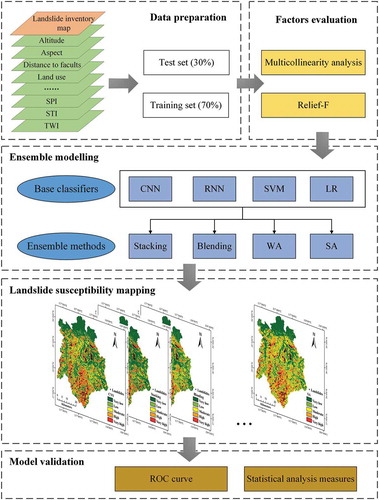
Figure 2 illustrates the flowchart of our heterogeneous ensemble-learning framework. First, we used historical landslide locations and selected conditioning factors to obtain training and test datasets, and then screened these factors via multicollinearity analysis and Relief-F. Next, we generated resultant susceptibility maps by using the proposed framework. Finally, we evaluated the performance of the proposed ensemble-learning methods based on the objective measures.

Figure 2. Flowchart of the heterogeneous ensemble-learning framework

3.1. Evaluation of conditioning factors

Feature selection is important in the field of data mining and has been widely used in LSM (Bui et al. 2016, Pourghasemi and Rahmati 2018). Irrelevant and extraneous features may have a negative impact on prediction performance. In this study, we used multicollinearity analysis and Relief-F feature selection methods to remove redundant factors.

3.1.1. Multicollinearity analysis

Multicollinearity analysis is used to assess the correlation between landslide conditioning factors. Multicollinearity means that the characteristics of at least two predicted features are highly correlated with linearity in multiple regression (Dormann et al. 2013). To objectively measure the multicollinearity results, two indicators of variance inflation factor (VIF) and tolerance (TOL) can be used. Specifically, if VIF >10 and TOL <0.1, the corresponding factor is multicollinear and should be excluded from the subsequent modelling process (Kavzoglu et al. 2014).

3.1.2. Relief-F

The Relief-F method can determine the relative importance of the conditioning factors to landslide occurrence, and it evaluates the value of conditioning factors by considering the correlation between factors and categories (Kira and Rendell 1992). First, the Relief-F algorithm randomly selects a sample R from the training set D. Then, we use k-nearest neighbour samples with a sample label of R and different labels from R to construct sample sets H and M, respectively. For factor set A, the weight of the ith factor is calculated as follows:

(1) $w_i=w_i-\sum _{j=1}^k\frac{diff(A_i,R,H_i)}{mk}+\sum _{C\ne Class(R)}\{\frac{p(C)}{1-p[Class(R)]}\sum _{j=1}^k\frac{diff[A_i,R,M_j(C)]}{mk}\}$(1)

where C denotes the sample label, p(C) is the probability of class C, Class (R) represents the label of sample R, M_j (C) is the jth sample of class C, and diff (A_i, R, H_i) and diff (A_i, R, M_i (C)) are the distance functions. Finally, we obtain the factor importance after repeating this process m times.

3.2. Base classifiers

3.2.1. CNN

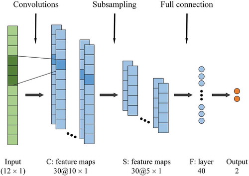
CNN can automatically learn useful features from hierarchical neural networks (LeCun et al. 2015). In this study, we used a one-dimensional CNN structure for landslide susceptibility prediction (Wang et al. 2019b, 2020a). In this case, the original landslide data are converted into a one-dimensional vector representation. The CNN architecture used in this study is shown in Figure 3. The hidden layers of CNN consists of a convolutional layer, a max pooling layer, and a fully connected layer, The convolutional layer uses a set of convolutional kernels to learn an effective representation from the input data. Let $v=\left\{v_1,v_2,\dots ,v_N\right\}$ be the input feature vectors, where N denotes the number of vectors. Assume that there are k kernels in the convolutional layer and the jth kernel has the weight and bias of w_j and b_j, respectively. First, output C_j of the convolutional operation is calculated as follows:

(2) $C_j=\sum _i^{N}f\left(w_j\ast v_i+b_j\right),j=1,2,\dots ,k$(2)

where f is the nonlinear activation function and * denotes the convolutional operator. Then, a pooling (sub-sampling) layer usually follows the convolutional layer to reduce the size of the feature vector, thereby avoiding the problem of overfitting. Max pooling is the most common pooling operation. When applying the max pooling operation (filter size of 2 and stride of 2), the length of the feature vectors is reduced by half, while the depth remains unchanged. Next, fully connected layers reorganize the extracted feature vectors. Finally, we use the softmax activation function to convert the reorganized vector into the predicted probability of the corresponding class. The probability is calculated as follows:

(3) $p\left(y=m\left|x\right.\right)=\frac{exp\left(w_{m}x+b_m\right)}{\sum _{n=1}^{M}exp\left(w_{n}x+b_n\right)}$(3)

where m represents the predicted class, M is the number of categories, w_m and w_n denote the weight vectors, and b_m and bn are the bias vectors.

Figure 3. Architecture of the CNN. C is for the convolutional layer, S is the subsampling layer, and F is the fully connected layer

3.2.2. RNN

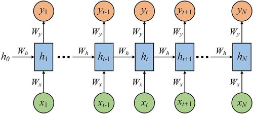
As a well-designed deep learning technique, RNN has received great attention in sequential data analysis tasks (Graves et al. 2013). It uses recurrent hidden states to process sequential inputs. These states can learn useful information not only from the current step but also from previous steps. This means that RNN has a powerful function to capture valuable information between sequence data. Therefore, it is highly important to construct a suitable landslide sequence representation for RNN modelling. In this study, based on the importance of landslide conditioning factors, we propose sequential representation for LSM in our previous study (Wang et al. 2020b). The structure of a typical RNN is shown in Figure 4. Let $x=\left\{x_1,x_2,\dots ,x_N\right\}$ be a sequence vector, $h=\left\{h_1,h_2\dots ,h_N\right\}$ a sequence of recurrent hidden state and $y=\left\{y_1,y_2\dots ,y_N\right\}$ a sequence of the output. For time step t,

(4) $h_t=f(W_x{x}_t+W_h{h}_{t-1}+b_h)$(4)

(5) $y_t=\phi (W_y{h}_t+b_y)$(5)

where f and φ are nonlinear activation functions, b_h and b_y denote the bias vectors, and W_x, W_h and W_y are the weight matrices shared in all time steps. The back-propagation through time algorithm continuously updates the weights until the RNN achieves satisfactory results.

Figure 4. Typical RNN architecture

3.2.3. SVM

SVM is a supervised machine learning model that uses a kernel trick to perform classification (Cortes and Vapnik 1995). For LSM, the purpose of SVM is to find a hyperplane that can properly distinguish between landslides and non-landslides. Assuming a training set$\mathbf{x}=\left\{x_1,x_2,...,x_N\right\}\in {\mathbb{R}}^{B\times N}$, the hyperplane can be minimized as follows:

(6) $\frac{1}{2}{∥\mathbf{w}∥}^2+C\sum _i{\xi }_i,s.t.y_i\left(\mathbf{w}\cdot x_i+b\right)\ge 1-{\xi }_i$(6)

where $∥\mathbf{w}∥$ represents the norm of the hyperplane normal, w is the weight vector, b denotes the bias, ${\xi }_i$ are the slack variables for non-separable data and C is the penalty parameter. The cost function is defined as follows:

(7) $\sum _{i=1}^n{\alpha }_i-\frac{1}{2}\sum _{i=1,j=1}^n{\alpha }_i{\alpha }_j{y}_i{y}_{j}K\left(x,x_i\right),s.t.0\le {\alpha }_i\le C,\sum _{i=1}^l{\alpha }_i{y}_i=0$(7)

where ${\alpha }_i$ are Lagrange multipliers and $K\left(x,x_i\right)$ is the kernel function. SVM with the radial basis function (RBF) kernel has been widely used in landslide susceptibility prediction (Pradhan 2013, Yu et al. 2016, Kumar et al. 2017), because RBF can achieve better performance than other kernels (Tehrany et al. 2015).

3.2.4. LR

LR is a supervised learning method that unusually uses logistic functions to solve binary classification problems. As a generalized linear regression model, LR has the advantages of simple implementation, high accuracy, and strong interpretation ability. Thus, it is the most commonly used statistical method in LSM (Reichenbach et al. 2018). The output prediction of LR is defined as follows (King and Zeng 2001):

(8) $p=\frac{1}{(1+e^{-z})}$(8)

where p is the probability and z denotes the linear combination of variables as follows:

(9) $z={\beta }_0+{\beta }_1{X}_1+{\beta }_2{X}_2+\cdot \cdot \cdot +{\beta }_N{X}_N$(9)

where $\left({\beta }_0,{\beta }_1,{\beta }_2,...,{\beta }_N\right)$ are the regression coefficients and$X=\left\{X_1,X_2,...,X_N\right\}$ represents the explanatory variables.

3.3. Ensemble-learning methods

3.3.1. Stacking

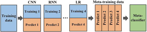
Stacking is a popular heterogeneous ensemble-learning technique that can use meta-models to combine different base classifiers for more accurate prediction results (Wolpert 1992). The flowchart of the stacking ensemble model is shown in Figure 5. The stacking method consists of the following steps: (1) use the training set to train different base classifiers through K-fold cross-validation; (2) collect the output predictions (feature vectors) of these base classifiers to generate a new reorganized training data set; (4) use the new training data set to train the meta-classifier. The stacking method can collectively estimate the errors of all base classifiers through basic learning steps and use meta-learning steps to reduce the prediction residuals.

Figure 5. Flowchart of stacking ensemble

3.3.2. Blending

Blending ensemble is a variation of the stacking ensemble originally introduced in the Netflix competition (Töscher and Jahrer 2009). The flowchart of the blending ensemble is shown in Figure 6. The blending method consists of the following steps: (1) use a hold-out method to divide the training set into a new training set and validation set; (2) use the new training set to train the base classifiers, and the prediction of the new validation set forms a meta-training dataset; (3) use the meta-training data to train the meta-classifier. Blending has a simpler structure than stacking and thus can avoid the problem of information leakage; however, blending is more likely to cause over-fitting.

Figure 6. Flowchart of blending ensemble

3.3.3. Averaging

Averaging is a common and simple ensemble-learning technique that has been successfully applied to natural disaster susceptibility mapping (Shafizadeh-Moghadam et al. 2018, Choubin et al. 2019). It consists of two ensemble-learning strategies of SA and WA. For SA, output prediction is the average of the probabilities of all base classifiers. Assuming that there are N base classifiers, the output probability of SA is calculated as follows:

(10) $p_{SA}=\frac{1}{N}\sum _{i=1}^N{p}_i$(10)

where P_i is the prediction probability of the ith base classifier.

For the WA ensemble, base classifiers are integrated using weighted averaging based on the area under the receiver operating characteristic (ROC) curve (AUC). The output prediction is defined as follows:

(11) $p_{WA}=\frac{AU{C}_j}{\sum _j^{N}AU{C}_j}{p}_j$(11)

where AUC_j and p_j denote the AUC value and the probability of the jth base classifier, respectively.

3.4. Model evaluation measures

In this study, we used the ROC curve (Bradley 1997) to assess the performance of the prediction model. The AUC value can effectively indicate the predictive capability of different LSM methods because it summarizes the performance of all possible decision boundaries (Reichenbach et al. 2018). In addition, six statistical measures of overall accuracy (OA), precision, recall, F-measure, Matthews correlation coefficient (MCC), and index of agreement (IOA) were used for evaluation:

(12) $OA=\frac{TP+TN}{TP+FP+TN+FN}$(12)

(13) $Precision=\frac{TP}{TP+FP}$(13)

(14) $Recall=\frac{TP}{TP+FN}$(14)

(15) $F-measure=\frac{2\times Precision\times Recall}{Precision+Recall}$(15)

(16) $MCC=\frac{TP\times TN-FP\times FN}{\sqrt{\left(TP+FP\right)\left(TP+FN\right)\left(TN+FP\right)\left(TN+FN\right)}}$(16)

(17) $IOA=1-\frac{\sum _{i=1}^n{\left(o_i-p_i\right)}^2}{\sum _{i=1}^n{\left(\left|o_i-\bar{o}\right|+\left|p_i-\bar{o}\right|\right)}^2}$(17)

where TP (true positive) and FP (false positive) are the number of samples correctly classified and misclassified as landslides, TN (true negative) and FN (false negative) are the number of samples correctly classified and misclassified as non-landslides, o_i and p_i are defined as true observations and predicted values, respectively, and $\bar{o}$ is the average of true observations.

4. Results

4.1. Factor assessment results

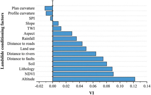
We used multicollinearity analysis to assess the correlation of landslide conditioning factors and reported the results in our previous publication (Wang et al. 2019b). The TOL and VIF values of STI did not meet the thresholds presented in Section 3.4. Therefore, the factor of STI was excluded from the subsequent analysis. The results of the Relief-F method are presented in Figure 7. Conditioning factors with higher variable importance (VI) values are more important for modelling, and factors with VI values less than zero indicate that these variables have no predictive ability. Figure 7 shows that the factor of altitude achieved the highest VI value. Moreover, the factors of plan curvature, profile curvature, and SPI had a VI value less than zero, meaning that these factors are not related to the occurrence of landslides and should be excluded from the modelling process.

Figure 7. Variable importance of each landslide conditioning factor using Relief-F

4.2. Construct of landslide models

We constructed four heterogeneous ensemble-learning methods by integrating CNN, RNN, SVM, and LR models. To construct training and test sets, we used a common sampling strategy (Eker et al. 2015, Bui et al. 2016, Jaafari et al. 2019), i.e. 70% of the landslides (266) were randomly selected for training, and the remaining 30% (114) for testing. Meanwhile, the same number of non-landslides (266 and 144) were randomly selected from areas without landslides to construct the training and test datasets. Note that the calculated hyperparameters of the landslide model are important for the final susceptibility results. In our experiments, we used the five-fold cross-validation procedure based on the training dataset to find the optimal hyperparameters of the landslide model. Specifically, we used the grid search procedure to adjust the hyperparameters of SVM and LR, and the search space was determined based on the previous studies (Ghorbanzadeh et al. 2019, Yang and Cervone 2019). As for the deep learning models of CNN and RNN, we used a common optimization process based on previous studies and the fine-tuning procedure (Hajimoradlou 2019, Sameen et al. 2019, Mutlu et al. 2019). For the stacking and blending methods, the LR model was the meta-classifier for final susceptibility prediction because simple linear models typically work well (Witten et al. 2016). Figure 8 shows the results of the analysis of two key hyperparameters of stacking and blending. The stacking ensemble-learning method obtained the highest AUC value when performing the three-fold cross-validation during the modelling process. When the ratio of the hold-out validation set is 0.5, the blending method can obtain the best results. All the hyperparameter settings in our experiments are presented in Table A1 in Appendix. The WA and SA ensemble-learning methods had no other hyperparameters. Modelling was performed in Python under two open frameworks of Keras⁵ and Scikit-Learn.⁶

Figure 8. Hyperparameter analysis of (a) stacking and (b) blending methods

4.3. Landslide susceptibility maps

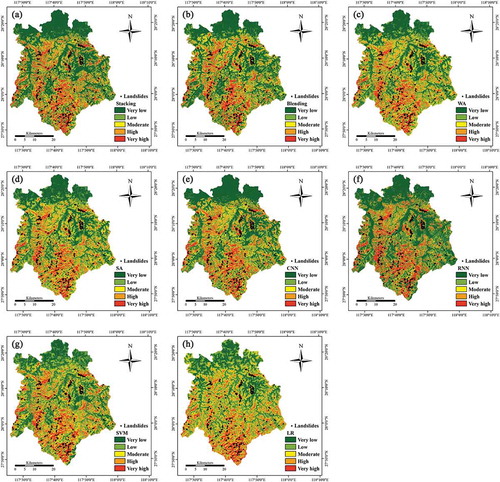
Once the LSM methods are constructed, the landslide model can calculate the susceptibility index of each grid cell. In this study, we reclassified all susceptibility indices into five categories: very high, high, moderate, low, and very low using the natural breaks method (Erener et al. 2016, Othman et al. 2018, Alizadeh et al. 2018). Figure 9 shows the landslide susceptibility maps using different methods. All the methods have a similar spatial distribution, i.e. most historical landslide locations are located in very high susceptibility areas. The very low susceptibility areas are mainly distributed in the northern part of the study area with low altitude and low slope.

Landslide density (LD) can quantitatively reflect the spatial distribution of obtained landslide susceptibility maps defined as the percentage of landslide pixels (PLP) divided by the percentage of susceptible class pixels (PSP). Table A2 in Appendix lists the detailed results of the LD analysis obtained using different methods. The very high susceptibility class obtained the highest LD value, followed by the high, moderate, low, very low susceptibility classes, indicating the reliability of the resultant susceptibility maps. Furthermore, the four heterogeneous ensemble-learning methods achieved higher LD values for the very high and high susceptibility classes than the base classifiers. The SA method achieved the highest LD value (5.77) for the very high and high susceptibility classes, while the LR method achieved the lowest value (4.67).

Figure 9. Landslide susceptibility maps by heterogeneous ensemble-learning methods of (a) Stacking, (b) Blending, (c) WA and (d) SA and base classifiers of (e) CNN, (f) RNN, (g) SVM, and (h) LR

4.4. Model validation and comparison

The prediction accuracy of the LSM methods using the test dataset is presented in Table 1. The heterogeneous ensemble-learning methods showed better performance than the base classifiers. The blending method achieved the highest OA value of 80.70%, followed by stacking (79.39%), WA and SA (78.07%), CNN and SVM (76.32%), RNN (75.44%), and LR (69.73%). Furthermore, we observed a similar trend in terms of MCC and IOA and blending achieved the best performance, followed by stacking, WA and SA, CNN, SVM, RNN and LR. Note that the WA and SA methods had the same values of these evaluation measures.

Table 1. Prediction accuracy of different prediction methods

	Methods	OA	Precision	Recall	F-measure	MCC	IOA
Ensemble-learning methods	Stacking	79.39%	0.7680	0.8421	0.8033	0.5905	0.7924
	Blending	80.70%	0.7966	0.8246	0.8103	0.6144	0.8068
	WA	78.07%	0.7667	0.8070	0.7863	0.5622	0.7802
	SA	78.07%	0.7667	0.8070	0.7863	0.5622	0.7802
Base classifiers	CNN	76.32%	0.7542	0.7807	0.7672	0.5266	0.7629
	RNN	75.44%	0.7589	0.7456	0.7522	0.5089	0.7543
	SVM	76.32%	0.7360	0.8070	0.7699	0.5199	0.7571
	LR	69.73%	0.6923	0.7105	0.7013	0.3949	0.6972

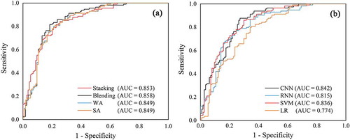
The ROC curves of different methods using the test set are shown in Figure 10. All the ensemble-learning methods showed better prediction performance than the base classifiers. For ensemble-learning, the blending method reached the highest AUC value (0.858), followed by stacking (0.853), and WA and SA (0.849). Regarding the base classifiers, CNN and LR reached the highest and lowest AUC values, respectively.

Figure 10. ROC curves of different methods using the test set (a) ensemble-learning methods and (b) base classifiers

4.5. Sensitivity analysis

To evaluate the sample sensitivity of the ensemble-learning methods, we generated a training set ranging from 10% to 90% with a step size of 10% for landslide susceptibility prediction. Table 2 lists the changes in the AUC values calculated using the test dataset. The heterogeneous ensemble-learning methods maintained better prediction performance than the base classifiers in most cases. Increasing the percentage of the training set from 10% to 70% resulted in an increase in the AUC of the ensemble-learning methods. Among the base classifiers, SVM maintained relatively good performance at different percentages, while LR always had the lowest AUC value.

Table 2. AUC variations with different percentages of the training set

	Methods	Percentage of training set (%)
		10	20	30	40	50	60	70	80	90
Ensemble-learning methods	Stacking	0.742	0.775	0.798	0.821	0.819	0.832	0.853	0.847	0.820
	Blending	0.774	0.792	0.786	0.817	0.814	0.839	0.858	0.850	0.834
	WA	0.763	0.786	0.818	0.826	0.813	0.831	0.849	0.847	0.829
	SA	0.770	0.785	0.817	0.826	0.810	0.830	0.849	0.847	0.829
Base classifiers	CNN	0.756	0.779	0.791	0.808	0.811	0.826	0.843	0.839	0.807
	RNN	0.713	0.772	0.775	0.803	0.801	0.820	0.815	0.835	0.805
	SVM	0.770	0.769	0.798	0.810	0.795	0.820	0.836	0.829	0.813
	LR	0.725	0.726	0.746	0.752	0.746	0.741	0.774	0.745	0.800

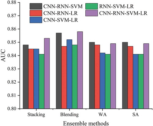
To identify the base classifier that can effectively help the ensemble-learning methods for LSM, ablation experiments were conducted. Figure 11 shows the AUC values of the ensemble-learning methods with three base classifiers. The stacking and blending methods that integrate all the base classifiers had higher AUC values than the three base classifiers. Moreover, the WA and SA methods that integrate CNN, RNN, and SVM had higher AUC values than the ensembles integrating all the base classifiers, indicating that LR has a negative impact on the WA and SA ensembles. Specifically, the AUC values of the stacking and WA methods demonstrated the greatest reduction without CNN, which means that CNN is an important component of these two ensemble-learning methods. For blending, SVM plays the most critical role in achieving good performance. For SA, CNN and RNN are equally important in the ensemble structure.

Figure 11. Results of base classifier ablation experiments

5. Discussion

Landslide susceptibility analysis is key for landslide disaster management and assessment (Reichenbach et al. 2018). Meanwhile, it is important to improve the performance of the prediction methods for managers and decision makers to obtain more accurate landslide susceptibility maps. To this end, this study integrates the popular deep learning methods of CNN and RNN with the conventional SVM and LR for LSM by using four heterogeneous ensemble-learning techniques of stacking, blending, WA, and SA.

In general, morphological, geological, and hydrological conditions are highly correlated with landslide occurrence (Yu et al. 2016, Jaafari et al. 2019, Pourghasemi et al. 2019). Therefore, it is necessary to analyse the effectiveness of landslide conditioning factors. In this study, using the Relief-F method, we found that altitude is the most critical conditioning factor because it determines the stress distribution of the slope. Meanwhile, it indirectly reflects human activities that may cause landslides. These observations are consistent with the previous studies (Tsangaratos and Ilia 2016, Pourghasemi and Rahmati 2018). Once the landslide conditioning factors are screened, we can construct the heterogeneous ensemble-learning methods for the spatial prediction of the landslide. The experimental results demonstrated that the ensemble-learning methods achieved higher prediction accuracies than the base classifiers because the ensemble strategy can better avoid the problem of overfitting and reduce bias and discrepancy (Shirzadi et al. 2017, Pham et al. 2018, Truong et al. 2018). On the other hand, the heterogeneous ensemble-learning techniques can learn the base classifiers with different perspectives from the hypothesis space, and thus they are expected to obtain more accurate prediction results than each individual base classifier.

The stacking and blending ensembles achieved higher prediction performance than other ensembles because they use meta-classifiers to correct the errors of the specific aspects that occur during the learning process of the base classifiers to improve the robustness and accuracy. Note that blending can achieve higher accuracy than stacking because information leakage may occur during the K-fold cross-validation process of stacking.

The averaging ensemble-learning methods of WA and SA achieved similar prediction results because WA uses AUC values as weights to combine different base classifiers, and the four base classifiers used in this study have small differences in AUC, resulting in similar weights. For example, the calculated weights were 0.2577, 0.2495, 0.2559, and 0.2369. Although WA may not achieve higher accuracy than blending, its use is still recommended to integrate different base classifiers for LSM due to its simple structure and no redundant hyperparameters. Moreover, WA is more suitable than SA to combine these models with significant performance differences. Shafizadeh-Moghadam et al. (2018) used seven ensemble forecasting techniques for flood susceptibility prediction and demonstrated that the performance of WA is higher than that of all base classifiers, ranking second among all the ensembles, which was also confirmed in our study.

Recently, Dou et al. (2019) integrated SVM models by using the stacking ensemble-learning technique for landslide susceptibility prediction and indicated that the performance of SVM cannot be improved by using the stacking technique. However, our study confirmed that stacking can improve the accuracy of base classifiers because four different base classifiers were selected for integration in our experiments, which increased the internal diversity of the stacking model, thereby reducing the bias and variance. We also implemented a hyperparameter optimization process shown in Figure 8 to ensure excellent performance of stacking.

The results of the sample sensitivity analysis showed that the heterogeneous ensemble-learning framework can generate more robust landslide models and provide reliable landslide susceptibility maps for decision makers. Moreover, the LD analysis to analyse the effectiveness of the landslide susceptibility maps assumes that the very high susceptibility area should have the densest landslide distribution, and the low susceptible area should have a lower landslide density (Ko and Lo 2018). The experimental results showed that the LD value increases from the very low susceptibility class to the very high susceptibility class, which is consistent with the results of the recent studies (Aditian et al. 2018, Jaafari et al. 2019). The proposed ensemble-learning methods also obtained higher LD values for the very high susceptibility area than the base classifiers because they can accurately predict the landslide area as a very high susceptibility area. The LD value of the very low susceptibility area is also a key indicator because predicting a potentially dangerous area as safe would lead to severe disasters. The results show that the LD value obtained by the ensemble-learning methods is lower than that obtained by the base classifiers in the very low susceptibility area. Therefore, the performance improvement brought by the heterogeneous ensemble-learning techniques is instructive for decision makers to analyse landslide susceptibility based on the heuristic experimental results.

6. Conclusions

The main objective of this study is to develop and compare four heterogeneous ensemble-learning methods that integrate CNN, RNN, SVM, and LR models for LSM. The proposed methods can capture the advantages of base classifiers by using different ensemble-learning strategies. The main conclusions based on the experimental results are summarized as follows. (1) The heterogeneous ensemble-learning methods can accurately characterize the distribution of regional landslide susceptibility. (2) The heterogeneous ensemble-learning techniques can effectively improve the predictive ability of the base classifiers. Specifically, the blending method achieved the highest prediction accuracies with OA and AUC of 80.70% and 0.858, respectively. (3) The ensemble-learning methods can stably achieve higher accuracies than the base classifiers when using different percentages of the training set. (4) The WA ensemble is the most recommended one for LSM because of its high accuracy and simple structure. Therefore, the heterogeneous ensemble-learning methods are effective in analysing the regional landslide susceptibility in other landslide-prone areas with a similar geological environment. This study provides an efficient method to combine different types of landslide susceptibility models and obtain more reliable susceptibility maps. Our future research will focus on exploring more effective ensemble-learning techniques and deep learning methods in landslide susceptibility analysis.

Abbreviations

The following abbreviations are used in this manuscript

AUC	=	Area under the ROC curve
CNN	=	Convolutional neural network
IOA	=	Index of agreement
LD	=	Landslide density
LR	=	Logistic regression
LSM	=	Landslide susceptibility mapping
MCC	=	Matthews correlation coefficient
NDVI	=	Normalized difference vegetation index
OA	=	Overall accuracy
PLP	=	Percentage of landslide pixels
PSP	=	Percentage of susceptible class pixels
RBF	=	Radial basis function
RNN	=	Recurrent neural network
ROC	=	The receiver operating characteristic curve
SPI	=	Stream power index
STI	=	Sediment transport index
SVM	=	Support vector machine
SA	=	Simple averaging
TOL	=	Tolerance
TWI	=	Topographic wetness index
VI	=	Variable importance
VIF	=	Variance inflation factor
WA	=	Weighted averaging

Acknowledgments

The authors would like to thank the handling editors and the three anonymous reviewers for their valuable comments and suggestions, which significantly improved the quality of this paper.

Disclosure statement

No potential conflict of interest was reported by the author(s).

Data and codes availability statement

The data and codes that support the findings of this study are available in GitHub at https://github.com/xmblb/HeterogeneousEnsemble.git.

Additional information

Funding

This work was supported by the National Natural Science Foundation of China [61271408, 41602362] and the China Scholarship Council [201906860029].

Notes on contributors

Zhice Fang

Zhice Fang is currently a Ph.D. candidate at the Institute of Geophysics and Geomatics of the China University of Geosciences, Wuhan. His research interests include natural disaster susceptibility mapping as well as remote sensing applications.

Yi Wang

Yi Wang is currently a professor at the Institute of Geophysics and Geomatics, China University of Geosciences (CUG), Wuhan. He received the B.S. degree in printing engineering and the Ph.D. degree in photogrammetry and remote sensing from Wuhan University, Wuhan, China, in 2002 and 2007, respectively. He is the head of the department of Geoinformatics and is a member of the IEEE, Chinese Association of Automation (CAA) and Geological Society of China (GSC). In 2019, he was named CUG Outstanding Young Talent. His research interests include remote sensing technology and application, Geoinformation data mining and Environmental impact assessment.

Ling Peng

Ling Peng is currently a senior engineer at the China Institute of Geo-Environment Monitoring, Beijing, China. He received the Ph.D. degree in Earth Exploration and Information Technology from China University of Geosciences, China, in 2013. His research interests include remote sensing applications for Geo-hazard prevention and Geo-environment protection.

Haoyuan Hong

Haoyuan Hong is currently a Lecturer of Geomorphology at the department of Geography and Regional Research, University of Vienna. He received the B.S. degree in geographic information system and the M.S. degree in climate system and global change from Nanjing University of Information Science and Technology, Nanjing, China, in 2007 and 2011, respectively. His research interests include machine learning, geographic information system and natural hazard assessment.

Notes

1. https://www.emdat.be

2. http://jx.cma.gov.cn

3. http://www.cgs.gov.cn

4. http://jx.cma.gov.cn

5. https://keras.io

6. https://scikit-learn.org

Appendix

Table A1. Hyperparameters setting of different prediction methods

	Methods	Hyperparameters	Search space	Final settings
Base classifiers	CNN	Convolutional kernel size	None	3 × 1
		Number of convolution unit		30
		Max pooling kernel size		2 × 1
		Number of epochs		150
		Activation function		ReLU
		Optimizer		Adamax
		Learning rate		0.002
		Dropout rate		0.2
	RNN	Number of recurrent units	None	30
		Number of epochs		150
		Activation function		ReLU
		Optimizer		RMSprop
		Learning rate		0.001
		Dropout rate		0.2
	SVM	Gamma	[10, 1, 0.1, 0.001, 0.0001]	0.001
		C	[0.1, 1, 10, 1000]	1000
	LR	Penalty	[‘l1ʹ, ‘l2ʹ]	l2
		C	[0.001, 0.01, 0.1, 1, 10, 100]	0.1
Ensemble-learning methods	Stacking	Fold of cross-validation	[2, 3, 4, 5, 6, 7, 8, 9, 10]	3
	Blending	Ratio of hold-out validation set	[0.1,.0.2, 0.3, 0.4, 0.5, 0.6, 0.7, 0.8, 0.9]	0.5

Table A2. Density analysis of resultant susceptibility maps by different prediction models

	Methods	Susceptibility class	No. of class pixels	No. of landslide pixels	PSP	PLP	LD
Ensemble-learning methods	Stacking	Very low	1,402,022	15	40.48	3.95	0.10
		Low	637,127	26	18.40	6.84	0.37
		Moderate	462,161	50	13.34	13.16	0.99
		High	505,874	85	14.61	22.37	1.53
		Very high	456,269	204	13.17	53.68	4.08
	Blending	Very low	1,295,392	14	37.40	3.68	0.10
		Low	744,365	39	21.49	10.26	0.48
		Moderate	519,316	60	14.99	15.79	1.05
		High	449,272	94	12.97	24.74	1.91
		Very high	455,108	173	13.14	45.53	3.46
	WA	Very low	1,082,987	10	31.27	2.63	0.08
		Low	811,923	25	23.44	6.58	0.28
		Moderate	612,480	57	17.68	15.00	0.85
		High	540,406	111	15.60	29.21	1.87
		Very high	415,657	177	12.00	46.58	3.88
	SA	Very low	1,092,710	11	31.55	2.89	0.09
		Low	796,566	24	23.00	6.32	0.27
		Moderate	616,996	56	17.81	14.74	0.83
		High	542,450	113	15.66	29.74	1.90
		Very high	414,731	176	11.97	46.32	3.87
Base classifiers	CNN	Very low	1,285,363	20	37.11	5.26	0.14
		Low	646,979	22	18.68	5.79	0.31
		Moderate	550,601	56	15.90	14.74	0.93
		High	510,959	93	14.75	24.47	1.66
		Very high	469,551	189	13.56	49.74	3.67
	RNN	Very low	1,575,589	27	45.49	7.11	0.16
		Low	558,340	38	16.12	10.00	0.62
		Moderate	397,451	50	11.48	13.16	1.15
		High	407,235	71	11.76	18.68	1.59
		Very high	524,838	194	15.15	51.05	3.37
	SVM	Very low	976,996	8	28.21	2.11	0.07
		Low	820,357	26	23.69	6.84	0.29
		Moderate	631,043	55	18.22	14.47	0.79
		High	559,218	103	16.15	27.11	1.68
		Very high	475,839	188	13.74	49.47	3.60
	LR	Very low	836,474	17	24.15	4.47	0.19
		Low	881,535	41	25.45	10.79	0.42
		Moderate	763,186	84	22.04	22.11	1.00
		High	593,034	113	17.12	29.74	1.74
		Very high	389,224	125	11.24	32.89	2.93

References

- Aditian, A., Kubota, T., and Shinohara, Y., 2018. Comparison of GIS-based landslide susceptibility models using frequency ratio, logistic regression, and artificial neural network in a tertiary region of Ambon, Indonesia. Geomorphology, 318 (2018), 101–111. doi:10.1016/j.geomorph.2018.06.006.
- Akgun, A., Dag, S., and Bulut, F., 2008. Landslide susceptibility mapping for a landslide-prone area (Findikli, NE of Turkey) by likelihood-frequency ratio and weighted linear combination models. Environmental Geology, 54 (6), 1127–1143. doi:10.1007/s00254-007-0882-8.
- Alizadeh, M., et al., 2018. Social vulnerability assessment using artificial neural network (ANN) model for earthquake hazard in Tabriz city, Iran. Sustainability, 10 (10), 3376. doi:10.3390/su10103376.
- Althuwaynee, O.F., et al., 2014. A novel ensemble bivariate statistical evidential belief function with knowledge-based analytical hierarchy process and multivariate statistical logistic regression for landslide susceptibility mapping. Catena, 114, 21–36. doi:10.1016/j.catena.2013.10.011.
- Alvioli, M. and Baum, R.L., 2016. Parallelization of the TRIGRS model for rainfall-induced landslides using the message passing interface. Environmental Modelling and Software, 81, 122–135. doi:10.1016/j.envsoft.2016.04.002
- Anagnostopoulos, G.G., Fatichi, S., and Burlando, P., 2015. An advanced process‐based distributed model for the investigation of rainfall‐induced landslides: the effect of process representation and boundary conditions. Water Resources Research, 51 (9), 7501–7523. doi:10.1002/2015WR016909.
- Ayalew, L. and Yamagishi, H., 2005. The application of GIS-based logistic regression for landslide susceptibility mapping in the Kakuda-Yahiko Mountains, Central Japan. Geomorphology, 65 (1), 15–31. doi:10.1016/j.geomorph.2004.06.010.
- Ayalew, L., Yamagishi, H., and Ugawa, N., 2004. Landslide susceptibility mapping using GIS-based weighted linear combination, the case in Tsugawa area of Agano River, Niigata Prefecture, Japan. Landslides, 1 (1), 73–81. doi:10.1007/s10346-003-0006-9.
- Bradley, A.P., 1997. The use of the area under the ROC curve in the evaluation of machine learning algorithms. Pattern Recognition, 30 (7), 1145–1159. doi:10.1016/s0031-3203(96)00142-2.
- Bueechi, E., et al., 2019. Regional-scale landslide susceptibility modelling in the Cordillera Blanca, Peru—a comparison of different approaches. Landslides, 16 (2), 395–407. doi:10.1007/s10346-018-1090-1.
- Bui, D.T., et al., 2016. GIS-based modeling of rainfall-induced landslides using data mining-based functional trees classifier with AdaBoost, Bagging, and MultiBoost ensemble frameworks. Environmental Earth Sciences, 75 (14), 1101. doi:10.1007/s12665-016-5919-4.
- Chen, W., et al., 2019. Spatial prediction of landslide susceptibility using gis-based data mining techniques of anfis with whale optimization algorithm (woa) and grey wolf optimizer (gwo). Applied Sciences, 9 (18), 3755. doi:10.3390/app9183755.
- Chen, W., Panahi, M., and Pourghasemi, H. R., 2017. Performance evaluation of GIS-based new ensemble data mining techniques of adaptive neuro-fuzzy inference system (ANFIS) with genetic algorithm (GA), differential evolution (DE), and particle swarm optimization (PSO) for landslide spatial modelling. Catena, 157, 310–324. doi: 10.1016/j.catena.2017.05.034
- Choubin, B., et al., 2019. An Ensemble prediction of flood susceptibility using multivariate discriminant analysis, classification and regression trees, and support vector machines. Science of the Total Environment, 651, 2087–2096. doi:10.1016/j.scitotenv.2018.10.064.
- Ciurleo, M., Cascini, L., and Calvello, M., 2017. A comparison of statistical and deterministic methods for shallow landslide susceptibility zoning in clayey soils. Engineering Geology, 223, 71–81. doi:10.1016/j.enggeo.2017.04.023
- Collobert, R., and Weston, J., 2008. A unified architecture for natural language processing: deep neural networks with multitask learning. In: Proceedings of the 25th international conference on Machine learning. Helsinki, Finland: ACM, 160–167.
- Cortes, C. and Vapnik, V., 1995. Support-vector networks. Machine Learning, 20 (3), 273–297. doi:10.1007/BF00994018.
- Dietterich, T.G., 1997. Machine-learning research. Ai Magazine, 18 (4), 97. doi:10.1609/aimag.v18i4.1324.
- Dormann, C.F., et al., 2013. Collinearity: a review of methods to deal with it and a simulation study evaluating their performance. Ecography, 36 (1), 27–46. doi:10.1111/j.1600-0587.2012.07348.x.
- Dou, J., et al., 2019. Improved landslide assessment using support vector machine with bagging, boosting, and stacking ensemble machine learning framework in a mountainous watershed, Japan. Landslides. doi:10.1007/s10346-019-01286-5.
- Eker, A.M., et al., 2015. Evaluation and comparison of landslide susceptibility mapping methods: a case study for the Ulus district, Bartın, northern Turkey. International Journal of Geographical Information Science, 29 (1), 132–158. doi:10.1080/13658816.2014.953164.
- Erener, A., Mutlu, A., and Düzgün, H.S., 2016. A comparative study for landslide susceptibility mapping using GIS-based multi-criteria decision analysis (MCDA), logistic regression (LR) and association rule mining (ARM). Engineering Geology, 203, 45–55. doi:10.1016/j.enggeo.2015.09.007
- Fang, Z., et al., 2020. Integration of convolutional neural network and conventional machine learning classifiers for landslide susceptibility mapping. Computers & Geosciences, 139, 104470. doi:10.1016/j.cageo.2020.104470.
- Feizizadeh, B. and Blaschke, T., 2013. GIS-multicriteria decision analysis for landslide susceptibility mapping: comparing three methods for the Urmia lake basin, Iran. Natural Hazards, 65 (3), 2105–2128. doi:10.1007/s11069-012-0463-3.
- Galli, M., et al., 2008. Comparing landslide inventory maps. Geomorphology, 94 (3–4), 268–289. doi:10.1016/j.geomorph.2006.09.023.
- Ghorbanzadeh, O., et al., 2019. Evaluation of different machine learning methods and deep-learning convolutional neural networks for landslide detection. Remote Sensing, 11 (2), 196. doi:10.3390/rs11020196.
- Graves, A., Mohamed, A.-R., and Hinton, G., 2013. Speech recognition with deep recurrent neural networks. In: IEEE international conference on acoustics, speech and signal processing. Vancouver, BC, Canada: IEEE, 6645–6649.
- Guha-Sapir, D., Below, R., and Hoyois, P., 2020. EM-DAT: international disaster database. Brussels, Belgium: Université Catholique de Louvain. Available from: http://www.emdat.be [Accessed 3 March 2020].
- Guzzetti, F., et al., 1999. Landslide hazard evaluation: a review of current techniques and their application in a multi-scale study, Central Italy. Geomorphology, 31 (1–4), 181–216. doi:10.1016/S0169-555X(99)00078-1.
- Guzzetti, F., et al., 2006. Estimating the quality of landslide susceptibility models. Geomorphology, 81 (1–2), 166–184. doi:10.1016/j.geomorph.2006.04.007.
- Hajimoradlou, A., 2019. Predicting landslides using contour aligning convolutional neural networks. Thesis (PhD). University of British Columbia, Vancouver.
- Han, J., et al., 2018. Advanced deep-learning techniques for salient and category-specific object detection: a survey. IEEE Signal Processing Magazine, 35 (1), 84–100. doi:10.1109/msp.2017.2749125.
- Hong, H., et al., 2018. Landslide susceptibility mapping using J48 Decision Tree with AdaBoost, Bagging and Rotation Forest ensembles in the Guangchang area (China). Catena, 163, 399–413. doi:10.1016/j.catena.2018.01.005.
- Huang, F., et al., 2019. A deep learning algorithm using a fully connected sparse autoencoder neural network for landslide susceptibility prediction. Landslides, 17, 1–13. doi:10.1007/s10346-019-01274-9.
- Jaafari, A., et al., 2019. Meta optimization of an adaptive neuro-fuzzy inference system with grey wolf optimizer and biogeography-based optimization algorithms for spatial prediction of landslide susceptibility. Catena, 175, 430–445. doi:10.1016/j.catena.2018.12.033.
- Kavzoglu, T., Sahin, E.K., and Colkesen, I., 2014. Landslide susceptibility mapping using GIS-based multi-criteria decision analysis, support vector machines, and logistic regression. Landslides, 11 (3), 425–439. doi:10.1007/s10346-013-0391-7.
- King, G. and Zeng, L., 2001. Logistic regression in rare events data. Political Analysis, 9 (2), 137–163. doi:10.18637/jss.v008.i02.
- Kira, K. and Rendell, L., 1992. A practical approach to feature selection. In: International conference on machine learning. San Francisco (CA): Morgan Kaufmann, 249–256
- Ko, F.W. and Lo, F.L., 2018. From landslide susceptibility to landslide frequency: A territory-wide study in Hong Kong. Engineering Geology, 242, 12–22. doi:10.1016/j.enggeo.2018.05.001
- Kornejady, A., Ownegh, M., and Bahremand, A., 2017. Landslide susceptibility assessment using maximum entropy model with two different data sampling methods. Catena, 152, 144–162. doi:10.1016/j.catena.2017.01.010
- Korzh, O., et al., 2017. Stacking approach for CNN transfer learning ensemble for remote sensing imagery. In: 2017 Intelligent Systems Conference (IntelliSys). London, UK: IEEE, 599–608.
- Kumar, D., et al., 2017. Landslide susceptibility mapping & prediction using support vector machine for Mandakini River Basin, Garhwal Himalaya, India. Geomorphology, 295, 115–125. doi:10.1016/j.geomorph.2017.06.013.
- LeCun, Y., Bengio, Y., and Hinton, G., 2015. Deep learning. Nature, 521 (7553), 436. doi:10.1038/nature14539.
- Lee, J., Kim, J., and Ko, W., 2019a. Day-ahead electric load forecasting for the residential building with a small-size dataset based on a self-organizing map and a stacking ensemble learning method. Applied Sciences, 9 (6), 1231. doi:10.3390/app9061231.
- Lee, S., et al., 2019b. Sevucas: A novel gis-based machine learning software for seismic vulnerability assessment. Applied Sciences, 9 (17), 3495. doi:10.3390/app9173495.
- Lee, S. and Pradhan, B., 2007. Landslide hazard mapping at Selangor, Malaysia using frequency ratio and logistic regression models. Landslides, 4 (1), 33–41. doi:10.1007/s10346-006-0047-y.
- Li, L.-J., et al., 2010. Object bank: A high-level image representation for scene classification & semantic feature sparsification. In: Advances in Neural Information Processing Systems. Vancouver, Canada: MIT Press, 1378–1386
- Lombardo, L. and Mai, P.M., 2018. Presenting logistic regression-based landslide susceptibility results. Engineering Geology, 244, 14–24. doi:10.1016/j.enggeo.2018.07.019
- Mandal, S. and Mandal, K., 2018. Modeling and mapping landslide susceptibility zones using GIS based multivariate binary logistic regression (LR) model in the Rorachu river basin of eastern Sikkim Himalaya, India. Modeling Earth Systems and Environment, 4 (1), 69–88. doi:10.1007/s40808-018-0426-0.
- Manzo, G., et al., 2013. GIS techniques for regional-scale landslide susceptibility assessment: the Sicily (Italy) case study. International Journal of Geographical Information Science, 27 (7), 1433–1452. doi:10.1080/13658816.2012.693614.
- Mutlu, B., et al., 2019. An experimental research on the use of recurrent neural networks in landslide susceptibility mapping. ISPRS International Journal of Geo-Information, 8 (12), 578. doi:10.3390/ijgi8120578.
- Oh, H.-J. and Pradhan, B., 2011. Application of a neuro-fuzzy model to landslide-susceptibility mapping for shallow landslides in a tropical hilly area. Computers & Geosciences, 37 (9), 1264–1276. doi:10.1016/j.cageo.2010.10.012.
- Othman, A.A., et al., 2018. Improving landslide susceptibility mapping using morphometric features in the Mawat area, Kurdistan Region, NE Iraq: comparison of different statistical models. Geomorphology, 319, 147–160. doi:10.1016/j.geomorph.2018.07.018.
- Pham, B.T., et al., 2017. Hybrid integration of Multilayer Perceptron Neural Networks and machine learning ensembles for landslide susceptibility assessment at Himalayan area (India) using GIS. Catena, 149, 52–63. doi:10.1016/j.catena.2016.09.007.
- Pham, B.T., et al., 2018. A hybrid machine learning ensemble approach based on a radial basis function neural network and rotation forest for landslide susceptibility modeling: A case study in the Himalayan area, India. International Journal of Sediment Research, 33 (2), 157–170. doi:10.1016/j.ijsrc.2017.09.008.
- Pham, B.T., et al., 2019a. A novel hybrid approach of landslide susceptibility modelling using rotation forest ensemble and different base classifiers. Geocarto International, 1–25. doi:10.1080/10106049.2018.1559885.
- Pham, B.T., et al., 2019b. Landslide susceptibility modeling using reduced error pruning trees and different ensemble techniques: hybrid machine learning approaches. Catena, 175, 203–218. doi:10.1016/j.catena.2018.12.018.
- Pham, B.T. and Prakash, I., 2018. Machine learning methods of kernel logistic regression and classification and regression trees for landslide susceptibility assessment at part of Himalayan area, India. Indian Journal of Science and Technology, 11. doi:10.17485/ijst/2018/v11i12/99745.
- Pourghasemi, H.R., et al., 2019. Multi-hazard probability assessment and mapping in Iran. Science of the Total Environment, 692, 556–571. doi:10.1016/j.scitotenv.2019.07.203.
- Pourghasemi, H.R., Pradhan, B., and Gokceoglu, C., 2012. Application of fuzzy logic and analytical hierarchy process (AHP) to landslide susceptibility mapping at Haraz watershed, Iran. Natural Hazards, 63 (2), 965–996. doi:10.1007/s11069-012-0217-2.
- Pourghasemi, H.R. and Rahmati, O., 2018. Prediction of the landslide susceptibility: which algorithm, which precision? Catena, 162, 177–192. doi:10.1016/j.catena.2017.11.022
- Pradhan, B., 2013. A comparative study on the predictive ability of the decision tree, support vector machine and neuro-fuzzy models in landslide susceptibility mapping using GIS. Computers & Geosciences, 51, 350–365. doi:10.1016/j.cageo.2012.08.023
- Reichenbach, P., et al., 2018. A review of statistically-based landslide susceptibility models. Earth-science Reviews, 180, 60–91. doi:10.1016/j.earscirev.2018.03.001.
- Sameen, M.I. and Pradhan, B., 2019. Landslide detection using residual networks and the fusion of spectral and topographic information. IEEE Access, 7, 114363–114373. doi:10.1109/ACCESS.2019.2935761
- Sameen, M.I., Pradhan, B., and Lee, S., 2019. Application of convolutional neural networks featuring Bayesian optimization for landslide susceptibility assessment. Catena, 186, 104249. doi:10.1016/j.catena.2019.104249
- Sesmero, M.P., Ledezma, A.I., and Sanchis, A., 2015. Generating ensembles of heterogeneous classifiers using stacked generalization. Wiley Interdisciplinary Reviews. Data Mining and Knowledge Discovery, 5 (1), 21–34. doi:10.1002/widm.1143.
- Shafizadeh-Moghadam, H., et al., 2018. Novel forecasting approaches using combination of machine learning and statistical models for flood susceptibility mapping. Journal of Environmental Management, 217, 1–11. doi:10.1016/j.jenvman.2018.03.089.
- Shahri, A.A., et al., 2019. Landslide susceptibility hazard map in southwest Sweden using artificial neural network. Catena, 183, 104225. doi:10.1016/j.catena.2019.104225.
- Shirzadi, A., et al., 2017. Shallow landslide susceptibility assessment using a novel hybrid intelligence approach. Environmental Earth Sciences, 76 (2), 60. doi:10.1007/s12665-016-6374-y.
- Sörensen, R., Zinko, U., and Seibert, J., 2006. On the calculation of the topographic wetness index: evaluation of different methods based on field observations. Hydrology and Earth System Sciences Discussions, 10 (1), 101–112. doi:10.5194/hess-10-101-2006.
- Tehrany, M.S., et al., 2015. Flood susceptibility assessment using GIS-based support vector machine model with different kernel types. Catena, 125 (125), 91–101. doi:10.1016/j.catena.2014.10.017.
- Termeh, S.V.R., et al., 2018. Flood susceptibility mapping using novel ensembles of adaptive neuro fuzzy inference system and metaheuristic algorithms. Science of the Total Environment, 615, 438–451. doi:10.1016/j.scitotenv.2017.09.262.
- Töscher, A. and Jahrer, M., 2009. The BigChaos Solution to the Netflix Grand Prize [online]. Available from: https://www.netflixprize.com/assets/GrandPrize2009_BPC_BigChaos.pdf
- Truong, X., et al., 2018. Enhancing prediction performance of landslide susceptibility model using hybrid machine learning approach of bagging ensemble and logistic model tree. Applied Sciences, 8 (7), 1046. doi:10.3390/app8071046.
- Tsangaratos, P., et al., 2017. Applying information theory and GIS-based quantitative methods to produce landslide susceptibility maps in Nancheng County, China. Landslides, 14 (3), 1091–1111. doi:10.1007/s10346-016-0769-4.
- Tsangaratos, P. and Ilia, I., 2016. Comparison of a logistic regression and Naïve Bayes classifier in landslide susceptibility assessments: the influence of models complexity and training dataset size. Catena, 145, 164–179. doi:10.1016/j.catena.2016.06.004
- Ullo, S.L., et al., 2019. Landslide Geohazard assessment with convolutional neural networks using Sentinel-2 imagery data. In: IGARSS 2019-2019 IEEE International Geoscience and Remote Sensing Symposium. Yokohama, Japan: IEEE, 9646–9649.
- Wang, G., et al., 2011. A comparative assessment of ensemble learning for credit scoring. Expert Systems with Applications, 38 (1), 223–230. doi:10.1016/j.eswa.2010.06.048.
- Wang, Q., et al., 2017. Integration of information theory, K-means cluster analysis and the logistic regression model for landslide susceptibility mapping in the Three Gorges Area, China. Remote Sensing, 9 (9), 938. doi:10.3390/rs9090938.
- Wang, Y., et al., 2019c. Flood susceptibility mapping in Dingnan County (China) using adaptive neuro-fuzzy inference system with biogeography based optimization and imperialistic competitive algorithm. Journal of Environmental Management, 247, 712–729. doi:10.1016/j.jenvman.2019.06.102.
- Wang, Y., et al., 2019d. Stacking-based ensemble learning of decision trees for interpretable prostate cancer detection. Applied Soft Computing, 77, 188–204. doi:10.1016/j.asoc.2019.01.015.
- Wang, Y., et al., 2020a. Flood susceptibility mapping using convolutional neural network frameworks. Journal Of Hydrology, 582, 124482. doi:10.1016/j.jhydrol.2019.124482.
- Wang, Y., et al., 2020b. Comparative study of landslide susceptibility mapping with different recurrent neural networks. Computers & Geosciences, 138, 104445. doi:10.1016/j.cageo.2020.104445.
- Wang, Y., Duan, H., and Hong, H., 2019a. A comparative study of composite kernels for landslide susceptibility mapping: A case study in Yongxin County, China. Catena, 183, 104217. doi:10.1016/j.catena.2019.104217.
- Wang, Y., Fang, Z., and Hong, H., 2019b. Comparison of convolutional neural networks for landslide susceptibility mapping in Yanshan County, China. Science of the Total Environment, 666, 975–993. doi:10.1016/j.scitotenv.2019.02.263.
- Witten, I.H., et al., 2016. Data mining: practical machine learning tools and techniques. San Francisco: Morgan Kaufmann.
- Wolpert, D.H., 1992. Stacked generalization. Neural Networks, 5 (2), 241–259. doi:10.1016/s0893-6080(05)80023-1.
- Xiao, L., Zhang, Y., and Peng, G., 2018. Landslide susceptibility assessment using integrated deep learning algorithm along the China-Nepal Highway. Sensors, 18 (12), 4436. doi:10.3390/s18124436.
- Yalcin, A., 2008. GIS-based landslide susceptibility mapping using analytical hierarchy process and bivariate statistics in Ardesen (Turkey): comparisons of results and confirmations. Catena, 72 (1), 1–12. doi:10.1016/j.catena.2007.01.003.
- Yang, L. and Cervone, G., 2019. Analysis of remote sensing imagery for disaster assessment using deep learning: a case study of flooding event. Soft Computing, 23 (24), 13393–13408. doi:10.1007/s00500-019-03878-8.
- Yu, X., et al., 2016. A combination of geographically weighted regression, particle swarm optimization and support vector machine for landslide susceptibility mapping: a case study at Wanzhou in the Three Gorges Area, China. International Journal of Environmental Research and Public Health, 13 (5), 487. doi:10.3390/ijerph13050487.