Exact space–time prism of an activity program: bidirectional searches in multi-state supernetwork

ABSTRACT

Space–time prism (STP) modeling for activity programs with various realizations of activity chains has been a challenging research topic. This study claims that a bidirectional search scheme in a multi-state supernetwork is capable of pinpointing the exact STP of an activity program. The correctness and search space are first analyzed for the existing two-stage bidirectional search methods originally suggested for constructing trip-based STPs. Two simultaneous bidirectional search methods are further suggested. Travel time lower bounds based on A*, landmarks, and triangular inequalities are applied in goal-directed searches to reduce the search space. The small twists in formalism over the existing methods ensure accuracy and computational efficiency. The performances of the different search methods are compared for conducting activity programs in large networks.

KEYWORDS:

• Space–time prism
• multi-state supernetwork
• goal-directed search
• activity program

1. Introduction

It has been recognized that humans are subject to space–time constraints to engage in activities, which involves allocating limited available time to access activities sparsely distributed in space. As a central time geographic concept, space–time prism (STP) delimits the space–time opportunities that can be reached by a moving object given the anchor points or known spatiotemporal locations (Hägerstrand 1970, Miller 1991). In the context of human travel and activity participation, an STP delineates the subset of spatial opportunities at moments in time available to an individual. It is propositioned that the actual activity-travel behavioral patterns occur in different forms within action spaces delineated by spatiotemporal conditions. STP models are widely applied to measure accessibility, the ability for individuals to travel and participate in activities (Miller 2017). The STP offers a perspective of person-based accessibility different from place-based accessibility measures focusing on a macro level (Neutens et al. 2011, Neutens 2015). Thus, STP and its extensions have large implications for spatial and transport planning initiatives respecting person heterogeneity.

In a seminal STP model (Lenntorp 1976), the outer bounds of a prism are determined by the maximum attainable travel speed, time budget, physical distance between the anchors, and the minimum duration of a flexible activity that can be conducted at one of multiple locations. An STP figuratively defines the envelope of all possible space–time paths. The projection of the STP to the two-dimensional plane determines the potential path area (PPA) that contains the set of feasible spatial opportunities. As these input parameters only hold in an ideal situation, considerable attention has been paid to relaxing the conditions of the original STP model. While it is not straightforward to define the prism shape analytically for most extensions, the examination of access to a location in time is essential for STP modeling and applications. Regarding the temporal dimension, early efforts have been devoted to incorporating varied link travel speeds and location time windows in real transport networks (e.g. Kwan and Hong 1998). It is noteworthy that STP is also re-labeled as network-time prism (NTP) if it is constructed over transport networks. Many STP extensions were suggested to accommodate flexible space–time anchor points, uncertain travel speeds, acceleration limits, and unequal prism interiors, analogous to attaching prefixes to STPs, such as rough, reliable, kinetic, and probabilistic (e.g. Chen et al. 2013, Kuijpers et al. 2017, Song et al. 2017). To further enhance realism, several behavioral facets were also studied in the STP framework, such as interpersonal interactions, virtual mobility, and multimodality. Apart from time budget, other constraints related to monetary budget, transfer times, travel distance range were also considered (e.g. Mahmoudi et al. 2019). These STP derivatives require algorithmic refinements on path-finding and result in major revisions to the ideal action space. On the applied side, the model extensions have wide applications, for example, in measurements of space–time accessibility (e.g. Chen et al. 2017) and task-oriented information value (e.g. Hu et al. 2016).

Existing STP models have been predominantly concentrated on one episode of activity participation, which are referred to as trip-based STPs. Their applications in the presence of activity chains usually require known activity sequences in such a way that the trip-based STPs are constructed sequentially as building STP blocks. There have been only a few pioneering endeavors constructing the STPs for conducting multiple activities. Specifically, Chen and Kwan (2012) proposed an approach for location choice set formation considering multiple flexible activities with flexible sequences between two anchors. To check the space–time constraints, their approach enumerates all feasible activity patterns to evaluate the accessible locations. Focusing on a general activity program (AP) of multiple activities, Kang and Chen (2016) generated the feasible space–time region by first uniting all location-specific space–time regions belonging to an activity and then intersecting all activity-specific space–time regions belonging to the AP. As summarized in Liao (2019), these three approaches have shortcomings (illustrated in Part 1 of the supplementary document). First, the way of building STP blocks tends to underestimate the overall STP since fixed activity sequencing unfavorably eliminates STP fractions associated with other activity sequences. Second, it is computationally inefficient to determine the accessible locations by plugging all location alternatives in enumerated activity patterns and calculating the shortest travel times between every two locations of different activities. Third, intersecting activity-specific space–time regions overestimates the overall STP because the feasible space–time regions of single activities are actually decreased after cumulating durations of multiple activities.

To accurately construct the STP for a generic AP, Liao (2019) suggested a novel search method. In the approach, multi-state supernetworks (Liao et al. 2010, 2011, 2013, 2014), defined as networks of networks at different states, were used to represent the path set of multi-activity travel patterns (see Section 2.2). A unidirectional goal-directed search method was proposed to find the path subset satisfying the temporal constraints. Naïve and tight bounds of activity-travel times from the search frontier to the anchor at the final activity state were formulated based on the method of ALT (A*, landmark, and triangular inequalities) (Goldberg and Harrelson 2005). The shortest activity-travel times through nodes outside the search space are considered larger than the time budget. The crust of the actual STP is supposed to lie in the area formed by excluding the lower bound STP from the upper bound STP (i.e. the ring area). Nonetheless, the approach of Liao (2019) has two drawbacks of creating the lower and upper bounds of activity-travel times. First, a buffer is created at the search frontier to limit the exploration of activity locations of unconducted activities. Second, a heuristic rule is used to create partial activity-travel patterns (ATPs) from the search frontier to the destination. These simplifications result in approximate STP bounds and thus imprecise STPs and PPAs.

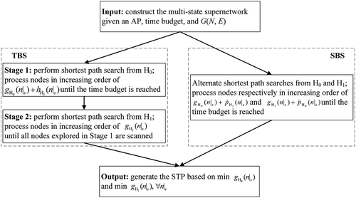
In view of the above, this study aims to suggest a bidirectional search scheme in a multi-state supernetwork for delineating the exact STP of an AP with flexible activity chains and test the efficiency of different bidirectional search methods. Three adaptations are suggested over the existing methods. First, the existing two-stage bidirectional search (TBS) methods (Kuijpers and Othman 2009, Chen et al. 2016) are applied in multi-state supernetworks. Second, the unidirectional search method using ALT (Liao 2019) is extended to TBS (referred to as TBS with ALT). Third, two simultaneous bidirectional search (SBS) methods for point-to-point (P2P) routing, i.e. finding the shortest path from one point (location) to another, are extended for constructing STPs in multi-state supernetworks (referred to as naïve SBS and SBS with ALT respectively; see Table 1 for the abbreviation list). All these adaptations lead to one common end, namely, bidirectional searches through a multi-state supernetwork. It is proved that all the above adaptations enable pinpointing the exact STP of an AP. Thus, the exact accessible locations and time ranges can be delineated. Compared with the two search methods with the first adaptation, TBS with ALT utilizes an advanced speedup technique that can significantly reduce search space and computation time. Compared with Liao (2019), TBS with ALT only uses strict lower bounds of ATP time expenses and obviates creating heuristic partial ATPs, which can guarantee accuracy and reduce computation time. These findings are verified by experimental examples using the same APs in large transport networks. It is unexpectedly found that SBS with ALT does not outperform TBS with ALT as it does in P2P routing and that the naïve SBS method excels in computation time when the time budget is slack.

Table 1. Abbreviations used in this study

STP: Space–time prism	AP: Activity program
PPA: Potential path area	ATP: Activity-travel pattern
NTP: Network-time prism	P2P: Point-to-point
TBS: Two-stage bidirectional search	ALT: A*, landmark, and triangular inequalities
SBS: Simultaneous bidirectional search	ALT*: ALT considering fixed activity location(s)

The remainder of this paper is organized as follows. Section 2 provides the preliminary knowledge of the existing TBS methods for constructing trip-based STPs and the unidirectional goal-directed search method in Liao (2019). Section 3 formally analyzes the correctness and search spaces of the TBS methods and presents a naïve and goal-directed SBS method. In Section 4, the bidirectional search scheme is demonstrated for conducting APs in large networks. Finally, this paper is completed with conclusions and a discussion of future work.

2. Preliminaries

This section provides the preliminary knowledge of two TBS methods for constructing trip-based STPs. The essences of multi-state supernetworks and the unidirectional goal-directed method are also briefly introduced to facilitate the development of TBS and SBS methods to construct the exact STP of an AP.

2.1. Speedup techniques for constructing trip-based STPs

Given flexible activity $\alpha$ with a minimum duration $d_{\alpha }$ and two anchor points ${\mathrm{H}}_0$ and ${\mathrm{H}}_1$ at time instances $t_0$ and $t_1$ ($t_0<t_1$) respectively, the conditions that location $n$ resides in the STP over the planar space and static transport network $G\left(N,E\right)$ with node set $N$ and link set $E$ are formulated as Equations (1(1) $e\left({\mathrm{H}}_0,n\right)+d_{\alpha }+e\left(n,{\mathrm{H}}_1\right)\le t_{\mathrm{B}}$(1) –2(2) $t\left({\mathrm{H}}_0,n\right)+d_{\alpha }+t\left(n,{\mathrm{H}}_1\right)\le t_{\mathrm{B}}$(2) ) respectively,

(1) $e\left({\mathrm{H}}_0,n\right)+d_{\alpha }+e\left(n,{\mathrm{H}}_1\right)\le t_{\mathrm{B}}$(1)

(2) $t\left({\mathrm{H}}_0,n\right)+d_{\alpha }+t\left(n,{\mathrm{H}}_1\right)\le t_{\mathrm{B}}$(2)

where $e\left(\cdot ,\cdot \right)$ denotes a lower bound travel time calculated as dividing the Euclidean distance between two nodes by the maximum travel speed (a dot represent an arbitrary node); $t\left(\cdot ,\cdot \right)$ denotes the shortest travel time between two nodes in $G$; thus, $e\left(\cdot ,\cdot \right)\le t\left(\cdot ,\cdot \right)$ (the arbitrary node pairs are the same); $t_{\mathrm{B}}$ is the time budget, $t_{\mathrm{B}}=t_1-t_0$. While one can solve Equation (1)(1) $e\left({\mathrm{H}}_0,n\right)+d_{\alpha }+e\left(n,{\mathrm{H}}_1\right)\le t_{\mathrm{B}}$(1) analytically, addressing Equation (2)(2) $t\left({\mathrm{H}}_0,n\right)+d_{\alpha }+t\left(n,{\mathrm{H}}_1\right)\le t_{\mathrm{B}}$(2) requires finding the shortest paths. Most algorithmic implementations involved running one-to-all shortest path searches from H₀ and H₁ separately by exploring $G$ twice completely. In case $G$ has unidirectional or asymmetric links, $t\left(n,{\mathrm{H}}_1\right)$ may not equal $t\left({\mathrm{H}}_1,n\right)$ and the one-to-all shortest path search from H₁ needs to be run in the reversed network of $G$.

Since accessible nodes by an individual to conduct $\alpha$ are usually a small part of $G$, Kuijpers and Othman (2009) suggested a speedup technique to construct the STP in a sub-network of $G$. The preprocessing step utilizes the planar PPA as an upper bound of the search space, which rules out network nodes and links outside the planar PPA. As a result, the one-to-all shortest path algorithm is run twice only in the area defined by Equation (1)(1) $e\left({\mathrm{H}}_0,n\right)+d_{\alpha }+e\left(n,{\mathrm{H}}_1\right)\le t_{\mathrm{B}}$(1) . However, it is argued that the computational gain is limited because the PPA in the planar space is considerably large compared with the counterpart in $G$ and the shortest path search frontiers should be bounded by $t_{\mathrm{B}}-d_a$ in principle.

To further narrow down the search space, Chen et al. (2016) proposed a one-way goal-directed TBS geo-computational algorithm. Specifically, A* search (Doran 1967) is first used in the forward shortest path search from ${\mathrm{H}}_0$. Given $n$ at the search frontier (implying that $t\left({\mathrm{H}}_0,n\right)$ is known), $t\left(n,{\mathrm{H}}_1\right)$ is estimated as $e\left(n,{\mathrm{H}}_1\right)$ to determine if $n$ must be outside the STP. The forward search space is delineated by Equation (3)(3) $t\left({\mathrm{H}}_0,n\right)+d_{\alpha }+e\left(n,{\mathrm{H}}_1\right)\le t_{\mathrm{B}}$(3) , which is a little ${\mathrm{H}}_1$-skewed since the share of $e\left(n,{\mathrm{H}}_1\right)$ gets less as $n$ approaches ${\mathrm{H}}_1$. In the backward shortest path search from ${\mathrm{H}}_1$, there is no need to estimate $t\left({\mathrm{H}}_0,n\right)$ as it is known earlier. 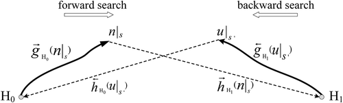Thus, the backward search space is delineated by Equation (2)(2) $t\left({\mathrm{H}}_0,n\right)+d_{\alpha }+t\left(n,{\mathrm{H}}_1\right)\le t_{\mathrm{B}}$(2) , which is tighter than Equaiton (3)(3) $t\left({\mathrm{H}}_0,n\right)+d_{\alpha }+e\left(n,{\mathrm{H}}_1\right)\le t_{\mathrm{B}}$(3) . Both directional searches do not need to explore the transport network completely. The schematic representation of the search spaces is given in Figure 1.

(3) $t\left({\mathrm{H}}_0,n\right)+d_{\alpha }+e\left(n,{\mathrm{H}}_1\right)\le t_{\mathrm{B}}$(3)

Figure 1. Schematic representation of search spaces. Node $n_i$ $\left(i=1,2,3\right)$ is at the border of a search space. The time expense of pattern H₀ – $n_i$ – H₁ is equal to $t_{\mathrm{B}}-d_a$

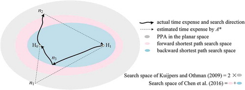
2.2. Multi-state supernetwork representation and goal-directed search

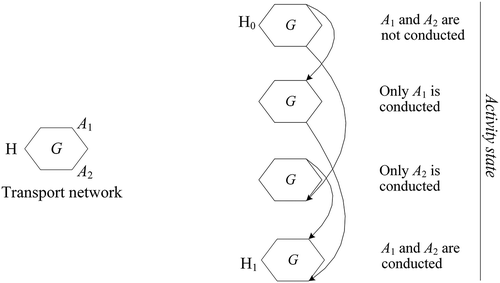
Multi-state supernetworks are powerful for representing ATPs of conducting an individual’s AP. The process of activity implementation is decomposed into path choice through a network of networks of differentiated states. In the context of STP modeling, which usually ignores multi-modal trip chaining, an activity state specifies which activities have been conducted. Considering all activity sequences, an AP of $\left|A\right|$ activities has $2^{\left|A\right|}$ activity states, where $A$ is the set of activities. Hence, a multi-state supernetwork has at most $2^{\left|A\right|}$ copies of the transport network, connected by unidirectional activity links at the same activity locations of different states. For example, Figure 2 shows a four-state supernetwork, in which activities A₁ and A₂ have one location alternative respectively at the angles of the hexagons denoting $G$. One may include more location alternatives by adding activity links connecting reachable states and more activities by adding more copies of $G$ based on activity sequences. Any path from ${\mathrm{H}}_0$ to ${\mathrm{H}}_1$ (origin and destination at the first and last states respectively, which may not be identical in $G$) is an ATP. The representation does not suffer from the curse of dimensionality since |A| is usually small in reality. Detailed explanations of terminologies and complexity analysis can be found in Liao et al. (2013) and Liao (2016).

Figure 2. Four-state supernetwork representation of conducting two activities (Liao 2019)

Without loss of generality, let $n{|}_s$denote node $n\in G$ at activity state $s$ in a multi-state supernetwork denoted by $SNK$. $SNK$ only shows the spatial action space and the temporal feasibility needs to be checked for a specific ATP. Similar to a trip-based STP, $n{|}_s$ resides in the STP over $SNK$ if it is in a path from H₀ to H₁ with activity-travel time no longer than $t_{\mathrm{B}}$. Liao (2019) formulated the temporal feasibility as Equation (4)(4) $min\left\{g_{{\mathrm{H}}_0}\left(n{|}_s\right)+g_{{\mathrm{H}}_1}\left(n{|}_s\right)\right\}\le t_{\mathrm{B}}$(4) and developed a unidirectional goal-directed search method using a potential function $f_{{\mathrm{H}}_0{\mathrm{H}}_1}(n{|}_s)$ to represent time expense of a path from ${\mathrm{H}}_0$ to ${\mathrm{H}}_1$ passing $n{|}_s$.

(4) $min\left\{g_{{\mathrm{H}}_0}\left(n{|}_s\right)+g_{{\mathrm{H}}_1}\left(n{|}_s\right)\right\}\le t_{\mathrm{B}}$(4)

(5) $f_{{\mathrm{H}}_0{\mathrm{H}}_1}(n{|}_s)=g_{{\mathrm{H}}_0}\left(n{|}_s\right)+h_{{\mathrm{H}}_1}\left(n{|}_s\right)$(5)

where $g_{{\mathrm{H}}_0}\left(n{|}_s\right)$ and $g_{{\mathrm{H}}_1}\left(n{|}_s\right)$ are the actual activity-travel times of sub-paths from ${\mathrm{H}}_0$ to $n{|}_s$ and $n{|}_s$ to ${\mathrm{H}}_1$ respectively; $h_{{\mathrm{H}}_1}\left(n{|}_s\right)$ is an estimation of $min{g}_{{\mathrm{H}}_1}\left(n{|}_s\right)$. Based on the ALT method and other heuristic rules, $min{g}_{{\mathrm{H}}_1}\left(n{|}_s\right)$ is estimated with tight lower and upper bounds. For ensuring sufficient exploration, a potential function with the naïve lower bound of $g_{{\mathrm{H}}_1}\left(n{|}_s\right)$ is applied to channel the goal-directed search. 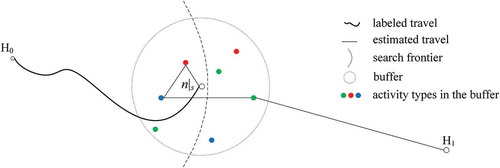During the path extension, approximate lower and upper bounds of $min{f}_{{\mathrm{H}}_0{\mathrm{H}}_1}(n{|}_s)$ are obtained to determine the temporal feasibility at $n{|}_s$. Figure 3 shows the two limitations at the search frontier $n{|}_s$ using the method of Liao (2019): (1) a buffer is created at $n{|}_s$ to limit the search area; (2) the classic nearest neighbor algorithm is applied to create the partial ATP from $n{|}_s$ to ${\mathrm{H}}_1$. Thus, the unidirectional goal-directed search method only outputs approximate state-dependent STPs.

Figure 3. Schematic representation at the search frontier $n{|}_s$ using the method of Liao (2019). The partial ATP from $n{|}_s$ to ${\mathrm{H}}_1$ has activity sequence red→blue→green

3. Exact STP of an AP

This section discusses a bidirectional search scheme for constructing the exact STP of an individual’s AP that includes one or more activities with any activity sequencing. As demonstrated in Section 2.2, multi-state supernetworks offer a generic way of representing the action space of ATPs. It is propositioned that the search methods and speedup techniques applicable to constructing trip-based STPs in $G$ are also applicable to constructing the STPs of APs in $SNK$.

The following part analyzes the correctness and the search spaces of existing TBS methods and newly-suggested SBS methods. The bidirectional searches are referred to as two-stage (TBS) if the search from one anchor is started only when that from the other anchor is completed, and as simultaneous (SBS) if the searches from two anchors are run in parallel. Within the search scheme, a TBS or SBS method can be goal-directed for accelerating the search process. A* and ALT are two common goal-directed speedup techniques (Bast et al. 2016). Accordingly, a TBS method using A* is referred to as TBS with A*, and a TBS method using ALT is referred to as TBS with ALT; other combinations can be defined similarly. In addition, a TBS or SBS method is called ‘naïve’ if no goal-directed technique is used.

To keep consistency, this study adopts the same setup as Liao (2019). Links in static transport network $G$ are travel links representing physical movement, activity locations are distributed at nodes of $G$, and all possible ATPs for conducting an AP are represented in $SNK$. The $SNK$ is a down-scaled representation that ignores multimodal trip chains (e.g. Figure 2). An individual travels with link-dependent maximum attainable speeds given a transport mode. A node in $G$ is attached with activity state information in $SNK$ by connector ‘|’, for instance, $n$ in $G$ and $n{|}_s$ in $SNK$, where $s$ is an element of the activity state set $S$. Let $l\left(\cdot ,\cdot \right)$ denote the (activity or travel) time expense of a link in $G$ or $SNK$. For travel link $\left(u,v\right)$, $l\left(u,v\right)=l\left(u{|}_s,v{|}_{s^{\prime }}\right)$ holds $\mathrm{\forall }s,s^{\prime }$. Activity links related to any activity $\alpha \in A$ take the minimum duration $d_a$ as the time expense. Denote the opening hours as time window $\left[o_{au},e_{au}\right]$, $d_{\alpha }+o_{\alpha u}\le e_{\alpha u}$, where $o_{\alpha u}$ and $e_{\alpha u}$ are the opening and closing times respectively at location alternative $u$ of $\alpha$. If conducting $\alpha$ at state $s$ results in a new state $s^{\prime }$, $\left(u{|}_s,u_{s{ }^{\mathrm{\prime }}}\right)$ is an activity link in $SNK$, i.e. $l\left(u{|}_s,u_{s{ }^{\mathrm{\prime }}}\right)=d_a$. Unless otherwise explained, the notational dentitions used in Section 2 remain unchanged (Table 2 shows the main notations).

Table 2. Notation list

$G\left(N,E\right)$	Transport network $G$ with $N$ and $E$ being the sets of nodes and links respectively
$n,u,v$	Nodes (locations) in $G$ ($n,u,v\in G$)
$\alpha$, $A$, $S$	An activity, activity set, and activity state set of an AP respectively
$SNK$	Multi-state supernetwork related to the AP
$s$, $s^{\prime }$	Two activity states ($s,s^{\prime }\in S$)
$A_s$	Sub-set of activities that are not conducted at state $s$, $A_s+\overline{A_s}=A$
$\left|\mathrm{\Delta }\right|$	Number of elements of an arbitrary set $\mathrm{\Delta }$ (e.g. $N$, $S$, $A$)
$d_{\alpha }$	Minimum activity duration of $\alpha$ ($\alpha \in A$)
$\left[o_{\alpha u},e_{\alpha u}\right]$	Time window for activity $\alpha$ at $u$
${\mathrm{H}}_0$, ${\mathrm{H}}_1$	Two anchor points in $G$ or $SNK$ (at the first and last activity state respectively)
${ }_0$, $t_1$	Time points at ${\mathrm{H}}_0$ and ${\mathrm{H}}_1$ respectively
$t_{\mathrm{B}}$	Time budget to conduct the AP, $t_{\mathrm{B}}=t_1-t_0$
${|}_s$	Activity state information attached to nodes of $G$
$l\left(\cdot ,\cdot \right)$	Static time expense of a link in $G$ or $SNK$
$t\left(\cdot ,\cdot \right)$	Shortest travel time between any two nodes in $G$, $t\left(\cdot ,\cdot \right)\ge 0$
e(,)	Lower bound of $t\left(\cdot ,\cdot \right)$ by the Euclidean distance and maximum speed
$ALT\left(\cdot ,\cdot \right)$	Lower bound of $t\left(\cdot ,\cdot \right)$ by the ALT method
$g_{v{{|}_s}^{\prime }}\left(n{|}_s\right)$	Actual activity-travel time of a sub-path from $v{|}_{s^{\prime }}$ to $n{|}_s$
$h_{v{|}_{s^{\prime }}}\left(n{|}_s\right)$	Lower bound of $g_{v{|}_{s^{\prime }}}\left(n{|}_s\right)$
$p_{v{|}_{s^{\prime }}}\left(n{|}_s\right)$	Consistent and feasible lower bound of $g_{v{|}_{s^{\prime }}}\left(n{|}_s\right)$
$f_{{\mathrm{H}}_0{\mathrm{H}}_1}(n{|}_s)$	Potential function of a path time expense from ${\mathrm{H}}_0$ to ${\mathrm{H}}_1$ passing $n{|}_s$
$\to ,\leftarrow$	Forward and backward directions respectively placed on the top of notations

3.1. TBS

Existing TBS methods for creating a trip-based STP over traditional transport network G include (i) combining two standard one-to-all shortest path searches, (ii) preprocessing using the planar PPA in addition to (i) (Kuijpers and Othman 2009), and (iii) combining one goal-directed search using A* and one standard shortest path search (Chen et al. 2016). This subsection provides the theoretical analysis of these three methods in $SNK$ to pinpoint the exact STP for an AP. The correctness and the illustration of search spaces are presented below.

Lemma 1: The exact STP of an AP can be constructed by combining twice one-to-all shortest path searches from ${\mathrm{H}}_0$ and ${\mathrm{H}}_1$ in $SNK$ respectively.

Proof. As G and activity links are static, $SNK$ is static. It is possible to slightly modify the one-to-all shortest path search to accommodate time window constraints. Considering a sub-path from ${\mathrm{H}}_0$ to $u{|}_s$ of time expense $g_{{\mathrm{H}}_0}\left(u{|}_s\right)$, extending the sub-path with travel link ($u{|}_s$, $v{|}_s$) leads to $g_{{\mathrm{H}}_0}\left(v{|}_s\right)=g_{{\mathrm{H}}_0}\left(u{|}_s\right)+l\left(u{|}_s,v{|}_s\right)$; extending the sub-path with activity link ($u{|}_s$, $u{|}_{s^{\prime }}$) leads to Equation (6)(6) $g_{{\mathrm{H}}_0}\left(u{|}_{s^{\prime }}\right)=\left\{\begin{array}{c}{d}_{\alpha }+max\left(t_0+g_{{\mathrm{H}}_0}\left(u{|}_s\right),o_{\alpha u}\right),t_0+g_{{\mathrm{H}}_0}\left(u{|}_s\right)+d_{\alpha }\le e_{\alpha u}\\ +\mathrm{\infty },else\end{array}\right.$(6)

(6) $g_{{\mathrm{H}}_0}\left(u{|}_{s^{\prime }}\right)=\left\{\begin{array}{c}{d}_{\alpha }+max\left(t_0+g_{{\mathrm{H}}_0}\left(u{|}_s\right),o_{\alpha u}\right),t_0+g_{{\mathrm{H}}_0}\left(u{|}_s\right)+d_{\alpha }\le e_{\alpha u}\\ +\mathrm{\infty },else\end{array}\right.$(6)

Despite time window constraints, time expense as the routing metric keeps the first-in-first-out property of $SNK$ intact. Thus, $min{g}_{{\mathrm{H}}_0}\left(n{|}_s\right)$, $\mathrm{\forall }n{|}_s$, can still be found in $SNK$. Since activity links are unidirectional, one can find $min{g}_{{\mathrm{H}}_1}\left(n{|}_s\right)$, $\mathrm{\forall }n{|}_s$, by running another modified one-to-all shortest path search from ${\mathrm{H}}_1$ after reversing the activity and travel links. Thereafter, it is trivial to obtain the time range at which $n{|}_s$ is inside the STP (Equaiton (4)(4) $min\left\{g_{{\mathrm{H}}_0}\left(n{|}_s\right)+g_{{\mathrm{H}}_1}\left(n{|}_s\right)\right\}\le t_{\mathrm{B}}$(4) ). $?$

Using binary heap, the standard label-setting algorithm has running time complexity $O\left(\left|N\right|\cdot \mathrm{l}\mathrm{o}\mathrm{g}\left|N\right|\right)$ in sparse $G$ ($O(\left|N\right|=O\left(\left|E\right|\right)$, where $\left|N\right|$ and $\left|E\right|$ are the numbers of nodes and links in $G$. Given at most $2^{\left|A\right|}$ copies of $G$ in $SNK$, there are $O\left(2^{\left|A\right|}\cdot \left|N\right|\right)$ nodes in $SNK$ in the worst case. When constructing the SNK for an AP, activity links are only added between activity location pairs at reachable activity states. Thus, the multi-state supernetwork is also a sparse network and the algorithm has running time complexity $O\left(2^{\left|A\right|}\cdot \left|N\right|\cdot log\left(2^{\left|A\right|}\cdot \left|N\right|\right)\right)$. After removing lower-order factors, the complexity is reduced to $O\left(2^{\left|A\right|}\cdot \left|N\right|\cdot log\left|N\right|\right)$. For each run, the method may not need to explore $SNK$ completely because the search frontier should be bounded by $t_{\mathrm{B}}$. Any activity duration should not be subtracted from $t_{\mathrm{B}}$ since activity links are explicitly represented and included during path extensions. As $t_{\mathrm{B}}$ is often large in the context of a daily AP, the search space tends to be large.

Applying the speedup technique of Kuijpers and Othman (2009) requires constructing the PPA in the planar space. However, it is not forthright to derive the PPA for an AP analytically due to the complexity of the geometrical inequalities. An upper bound PPA in the planar space can be formulated as Equation (7)(7) $e\left({\mathrm{H}}_0,n\right)+\sum _{\alpha \in A}{d}_{\alpha }+e\left(n,{\mathrm{H}}_1\right)\le t_{\mathrm{B}}$(7) by assuming all activities of $A$ can be conducted at all locations, which is an extension of Equation (1)(1) $e\left({\mathrm{H}}_0,n\right)+d_{\alpha }+e\left(n,{\mathrm{H}}_1\right)\le t_{\mathrm{B}}$(1) . Delimited by Equation (7)(7) $e\left({\mathrm{H}}_0,n\right)+\sum _{\alpha \in A}{d}_{\alpha }+e\left(n,{\mathrm{H}}_1\right)\le t_{\mathrm{B}}$(7) , those nodes and links outside the planar PPA must not be inside the STP. Likewise, the upper bound PPAs at all states are delimited by Equation (8)(8) $e\left({\mathrm{H}}_0,n{|}_s\right)+\sum _{\alpha \in A}{d}_{\alpha }+e\left(n{|}_s,{\mathrm{H}}_1\right)\le t_{\mathrm{B}},\mathrm{\forall }s$(8) .

(7) $e\left({\mathrm{H}}_0,n\right)+\sum _{\alpha \in A}{d}_{\alpha }+e\left(n,{\mathrm{H}}_1\right)\le t_{\mathrm{B}}$(7)

(8) $e\left({\mathrm{H}}_0,n{|}_s\right)+\sum _{\alpha \in A}{d}_{\alpha }+e\left(n{|}_s,{\mathrm{H}}_1\right)\le t_{\mathrm{B}},\mathrm{\forall }s$(8)

$e\left(\cdot ,\cdot \right)$, derived by the Euclidean distance and maximum travel speed, does not contain the activity state information. The PPAs are exactly the same at all activity states. Hence, one can pinpoint the exact STP according to Lemma 1. The finding is concluded as Corollary 1.

Corollary 1: The exact STP of an AP can be constructed by combining twice one-to-all shortest path searches from ${\mathrm{H}}_0$ and ${\mathrm{H}}_1$ respectively in a part of $SNK$ delimited by Equaiton (8)(8) $e\left({\mathrm{H}}_0,n{|}_s\right)+\sum _{\alpha \in A}{d}_{\alpha }+e\left(n{|}_s,{\mathrm{H}}_1\right)\le t_{\mathrm{B}},\mathrm{\forall }s$(8) .

Proof. Equaiton (8)(8) $e\left({\mathrm{H}}_0,n{|}_s\right)+\sum _{\alpha \in A}{d}_{\alpha }+e\left(n{|}_s,{\mathrm{H}}_1\right)\le t_{\mathrm{B}},\mathrm{\forall }s$(8) only eliminates nodes and links of $SNK$ that must not be in the STP. The preprocessing step reduces the search space without compromising optimality.

To apply the method of Chen et al. (2016) (i.e., TBS with A*), Equations (3)(3) $t\left({\mathrm{H}}_0,n\right)+d_{\alpha }+e\left(n,{\mathrm{H}}_1\right)\le t_{\mathrm{B}}$(3) and (2(2) $t\left({\mathrm{H}}_0,n\right)+d_{\alpha }+t\left(n,{\mathrm{H}}_1\right)\le t_{\mathrm{B}}$(2) ) need to be extended to include multiple activities for the forward and backward searches in $SNK$ respectively. The condition for the forward search space is written as Equation (9)(9) $min{g}_{{\mathrm{H}}_0}\left(n{|}_s\right)+\sum _{\alpha \in A_s}{d}_{\alpha }+e\left(n{|}_s,{\mathrm{H}}_1\right)\le t_{\mathrm{B}}$(9) , where $A_s$ is a sub-set of $A$ consisting of activities that are not conducted yet at $s$. In Equation (9)(9) $min{g}_{{\mathrm{H}}_0}\left(n{|}_s\right)+\sum _{\alpha \in A_s}{d}_{\alpha }+e\left(n{|}_s,{\mathrm{H}}_1\right)\le t_{\mathrm{B}}$(9) , $\sum _{\alpha \in A_s}{d}_{\alpha }+e\left({\mathrm{H}}_1,n{|}_s\right)$ is a lower bound of the shortest activity-travel time from $n{|}_s$ to ${\mathrm{H}}_1$, assuming that $n{|}_s$ is an activity location for $\mathrm{\forall }\alpha \in A_s$.

(9) $min{g}_{{\mathrm{H}}_0}\left(n{|}_s\right)+\sum _{\alpha \in A_s}{d}_{\alpha }+e\left(n{|}_s,{\mathrm{H}}_1\right)\le t_{\mathrm{B}}$(9)

The condition for the backward search space remains as Equation (4)(4) $min\left\{g_{{\mathrm{H}}_0}\left(n{|}_s\right)+g_{{\mathrm{H}}_1}\left(n{|}_s\right)\right\}\le t_{\mathrm{B}}$(4) . Similarly, Corollary 2 is drawn. It is also found that the backward search space is confined by the actual PPA, which can be easily proved by the method of contradiction.

Corollary 2: The exact STP of an AP can be constructed by applying the TBS with A* in $SNK$.

Proof. As $g_{{\mathrm{H}}_0}\left(n{|}_s\right)$ consists of the actual travel and participation of activities not in $A_s$, Equations (10(10) $e\left({\mathrm{H}}_0,n{|}_s\right)+\sum _{\alpha \in A}{d}_{\alpha }+e\left(n{|}_s,{\mathrm{H}}_1\right)\le min{g}_{{\mathrm{H}}_0}\left(n{|}_s\right)+\sum _{\alpha \in A_s}{d}_{\alpha }+e\left(n{|}_s,{\mathrm{H}}_1\right)$(10) –11(11) $\le min\left\{g_{{\mathrm{H}}_0}\left(n{|}_s\right)+g_{{\mathrm{H}}_1}\left(n{|}_s\right)\right\}$(11) ) always hold.

(10) $e\left({\mathrm{H}}_0,n{|}_s\right)+\sum _{\alpha \in A}{d}_{\alpha }+e\left(n{|}_s,{\mathrm{H}}_1\right)\le min{g}_{{\mathrm{H}}_0}\left(n{|}_s\right)+\sum _{\alpha \in A_s}{d}_{\alpha }+e\left(n{|}_s,{\mathrm{H}}_1\right)$(10)

(11) $\le min\left\{g_{{\mathrm{H}}_0}\left(n{|}_s\right)+g_{{\mathrm{H}}_1}\left(n{|}_s\right)\right\}$(11)

The right-hand sides of Equations (10(10) $e\left({\mathrm{H}}_0,n{|}_s\right)+\sum _{\alpha \in A}{d}_{\alpha }+e\left(n{|}_s,{\mathrm{H}}_1\right)\le min{g}_{{\mathrm{H}}_0}\left(n{|}_s\right)+\sum _{\alpha \in A_s}{d}_{\alpha }+e\left(n{|}_s,{\mathrm{H}}_1\right)$(10) –11(11) $\le min\left\{g_{{\mathrm{H}}_0}\left(n{|}_s\right)+g_{{\mathrm{H}}_1}\left(n{|}_s\right)\right\}$(11) ) refer to the forward and backward search conditions respectively, which are tighter than the planar PPA condition delimited by Equation (8)(8) $e\left({\mathrm{H}}_0,n{|}_s\right)+\sum _{\alpha \in A}{d}_{\alpha }+e\left(n{|}_s,{\mathrm{H}}_1\right)\le t_{\mathrm{B}},\mathrm{\forall }s$(8) . Thus, by comparison, Equations (9)(9) $min{g}_{{\mathrm{H}}_0}\left(n{|}_s\right)+\sum _{\alpha \in A_s}{d}_{\alpha }+e\left(n{|}_s,{\mathrm{H}}_1\right)\le t_{\mathrm{B}}$(9) and (4(4) $min\left\{g_{{\mathrm{H}}_0}\left(n{|}_s\right)+g_{{\mathrm{H}}_1}\left(n{|}_s\right)\right\}\le t_{\mathrm{B}}$(4) ) further eliminate nodes and links that are not in the STP without compromising optimality.

$\sum _{\alpha \in A_s}{d}_{\alpha }+e\left(n{|}_s,{\mathrm{H}}_1\right)$ is used above as a lower bound of $min{g}_{{\mathrm{H}}_1}\left(n{|}_s\right)$. Other forms of lower bound function, denoted by $h_{{\mathrm{H}}_1}\left(n{|}_s\right)$, are also feasible in the goal-directed TBS method (e.g. TBS with ALT). The smaller the gap between $min{g}_{{\mathrm{H}}_1}\left(n{|}_s\right)$ and $h_{{\mathrm{H}}_1}\left(n{|}_s\right)$, the less extra space is explored. Once $h_{{\mathrm{H}}_1}\left(n{|}_s\right)\ge 0$, goal-directed TBS tends to explore less space than the first two TBS methods. For completeness, the pseudo-code of goal-directed TBS methods is briefly presented as Pseudo-code 1. Figure 1 schematically demonstrates Corollary 1 and 2 when $\left|A\right|=1$. Due to the various realizations of activity chains when $\left|A\right|>1$, it is not straightforward to generalize the sharp differences of search spaces. The illustrative comparisons will be shown in Section 4.

Pseudo-code 1: Goal-directed TBS

1. input G, SNK, H₀, H₁, t_B;

2. stage 1: perform shortest path search from H₀ using $min\left\{g_{{\mathrm{H}}_0}\left(n{|}_s\right)+h_{{\mathrm{H}}_1}\left(n{|}_s\right)\right\}$ as the routing metric;

3. stop when Equation (9)(9) $min{g}_{{\mathrm{H}}_0}\left(n{|}_s\right)+\sum _{\alpha \in A_s}{d}_{\alpha }+e\left(n{|}_s,{\mathrm{H}}_1\right)\le t_{\mathrm{B}}$(9) is violated;

4. generate a search space Ω;

5. stage 2: perform shortest path search from H₁ using min g₁(n|_s) as the routing metric;

6. check $min\left\{g_{{\mathrm{H}}_0}\left(n{|}_s\right)+g_{{\mathrm{H}}_1}\left(n{|}_s\right)\right\}\le t_{\mathrm{B}}$ when n|_s is extracted from the queue;

7. stop when all nodes in Ω are explored;

8. output STP = $\left\{\left(n{|}_s,t\right)|n{|}_s\in SNK,t\in \left[t_0+min{g}_{{\mathrm{H}}_0}\left(n{|}_s\right),t_1-min{g}_{{\mathrm{H}}_1}\left(n{|}_s\right)\right]\right\}.$

3.2. SBS

A large body of P2P routing literature has shown that SBS and the combinations with other speedup techniques substantially outperform the standard one-to-all shortest path algorithm (Bast et al. 2016). Despite intensively discussed in the context of P2P routing, SBS has not been discussed for STP modeling thus far. In this subsection, two SBS methods (i.e., a naïve one and a goal-directed one) are suggested to create the exact STP in $SNK$ for an AP.

3.2.1. Naïve SBS

A naïve SBS method simultaneously runs one standard shortest path search from the origin (forward search) and another from the destination (backward search). For P2P routing, SBS aims to find only one shortest path and terminates when the search frontiers meet. Whereas, STP modeling aims to find all shortest paths satisfying Equation (4)(4) $min\left\{g_{{\mathrm{H}}_0}\left(n{|}_s\right)+g_{{\mathrm{H}}_1}\left(n{|}_s\right)\right\}\le t_{\mathrm{B}}$(4) . The algorithm should continue after the search frontiers meet since there may be multiple shortest paths even if $min{g}_{{\mathrm{H}}_0}\left({\mathrm{H}}_1\right)=t_{\mathrm{B}}$ (the STP is empty if $min{g}_{{\mathrm{H}}_0}\left({\mathrm{H}}_1\right)>t_{\mathrm{B}}$). For both search directions, let ${\vec{g}}_{{\mathrm{H}}_0}\left(n{|}_s\right)$ and ${\overleftarrow{g}}_{{\mathrm{H}}_1}\left(n{|}_s\right)$ denote the tentative shortest activity-travel times from ${\mathrm{H}}_0$ and ${\mathrm{H}}_1$ to $n{|}_s$ respectively. Two priority queues, $P{Q}_{\mathrm{F}}$ and $P{Q}_{\mathrm{B}}$, are used to store temporarily labeled nodes. When the top node from a queue is extracted, it is at the frontier in the corresponding search direction and becomes permanently labeled. Then, the tentative shortest activity-travel time becomes definitive. For example, if $n{|}_s$ is an extracted top node from $P{Q}_{\mathrm{F}}$, we have $t\left({\mathrm{H}}_0,n{|}_s\right)=min{\vec{g}}_{{\mathrm{H}}_0}\left(n{|}_s\right)$, vice-versa. Denote the shortest activity-travel times from ${\mathrm{H}}_0$ and ${\mathrm{H}}_1$ to the frontiers in the forward and backward directions by $to{p}_{\mathrm{F}}$ and $to{p}_{\mathrm{B}}$ respectively. The pseudo-code of the naïve SBS method is described as Pseudo-code 2.

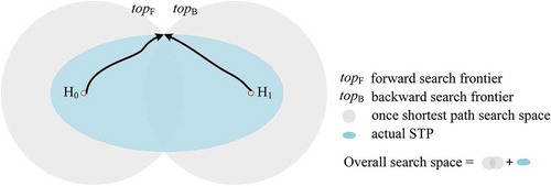
In the course of SBS, three distinctive phases are identified. In the first phase, before the two frontiers meet, i.e. $to{p}_{\mathrm{F}}+to{p}_{\mathrm{B}}<min{g}_{{\mathrm{H}}_0}\left({\mathrm{H}}_1\right)$, nodes are sequentially labeled permanently in one search direction while they are not even temporarily labeled in the opposite direction. Each frontier is extended in the same way as the standard shortest path search (lines 4–9). $PL\left(n{|}_s\right)=1$ means that $n{|}_s$ is permanently labeled in one reference search direction without differentiating forward or backward for ease of explanation, while $\overline{PL}\left(n{|}_s\right)=1$ means that $n{|}_s$ is permanently labeled in the opposite direction; otherwise, 0 means not permanently labeled.

Pseudo-code 2: Naïve SBS method

1. input $G$, $SNK$, ${\mathrm{H}}_0$, ${\mathrm{H}}_1$, $t_{\mathrm{B}}$; initialize ${\vec{g}}_{{\mathrm{H}}_0}\left(n{|}_s\right)={\overleftarrow{g}}_{{\mathrm{H}}_1}\left(n{|}_s\right)=+\mathrm{\infty }$, $\mathrm{\forall }n{|}_s$; ${\vec{g}}_{{\mathrm{H}}_0}\left({\mathrm{H}}_0\right)={\overleftarrow{g}}_{{\mathrm{H}}_1}\left({\mathrm{H}}_1\right)=0$;

2. insert label $⟨{\mathrm{H}}_0,{\vec{g}}_{{\mathrm{H}}_0}\left({\mathrm{H}}_0\right)⟩$ in $P{Q}_{\mathrm{F}}$ and $⟨{\mathrm{H}}_1,{\overleftarrow{g}}_{{\mathrm{H}}_1}\left({\mathrm{H}}_1\right)⟩$ in $P{Q}_{\mathrm{B}}$;

3. while $P{Q}_{\mathrm{F}}\ne \mathrm{\varnothing }$ and $P{Q}_{\mathrm{B}}\ne \mathrm{\varnothing }$

4. extract top nodes from $P{Q}_{\mathrm{F}}$ and $P{Q}_{\mathrm{B}}$ and label them permanently;

5. if $to{p}_{\mathrm{F}}+to{p}_{\mathrm{B}}\le t_{\mathrm{B}}$

6. for each neighboring node $u{|}_{s^{\prime }}$ of a top node with $PL\left(u{|}_{s{ }^{\mathrm{\prime }}}\right)=0$

7. update min ${\vec{g}}_{{\mathrm{H}}_0}\left(u{|}_{s^{\prime }}\right)$ or min ${\overleftarrow{g}}_{{\mathrm{H}}_1}\left(u{|}_{s^{\prime }}\right)$ and check if it decreases

8. insert or update the label in the corresponding queue;

9. end for

10. else

11. for each neighboring node $u{|}_{s^{\prime }}$ of a top node with $PL\left(u{|}_{s{ }^{\mathrm{\prime }}}\right)=0$ and $\overline{PL}\left(u{|}_{s{ }^{\mathrm{\prime }}}\right)=1$

12. update min ${\vec{g}}_{{\mathrm{H}}_0}\left(u{|}_{s^{\prime }}\right)$ or min ${\overleftarrow{g}}_{{\mathrm{H}}_1}\left(u{|}_{s^{\prime }}\right)$ and check if it decreases

13. insert or update the label in the corresponding queue;

14. end for

15. if top node $n{|}_s$ with $PL\left(n{|}_s\right)=\overline{PL}\left(n{|}_s\right)=1$ and $min\left\{{\vec{g}}_{{\mathrm{H}}_0}\left(n{|}_s\right)+{\overleftarrow{g}}_{{\mathrm{H}}_1}\left(n{|}_s\right)\right\}\le t_{\mathrm{B}}$

16. $n{|}_s$ at time range [$t_0+min{\vec{g}}_{{\mathrm{H}}_0}\left(n{|}_s\right),t_1-min{\overleftarrow{g}}_{{\mathrm{H}}_1}\left(n{|}_s\right)$] is inside the STP;

17. end while

18. output the STP.

In the second phase, $min{g}_{{\mathrm{H}}_0}\left({\mathrm{H}}_1\right)\le to{p}_{\mathrm{F}}+to{p}_{\mathrm{B}}\le t_{\mathrm{B}}$, only a fraction of nodes in the intersected area of the two searched areas is permanently labeled. Since it is premature to check the temporal feasibility of other nodes, the operations in this phase are the same as those in the first phase to guarantee sufficient exploration. In the third phase, $to{p}_{\mathrm{F}}+to{p}_{\mathrm{B}}>t_{\mathrm{B}}$, it signifies that any nodes outside the explored areas must not be in the STP. When extending the frontier in one search direction, the temporarily labeled nodes must have already been permanently labeled in the opposite search direction (lines 11–14). Once a node is newly labeled permanently, it must be labeled permanently in both search directions and it is trivial to check its temporal feasibility in the STP. Also, if a newly permanently labeled node is outside the PPA, it will not be considered for extending the frontier as it must not be in any path with a total activity-travel time less than or equal to $t_{\mathrm{B}}$. For that reason, the search space in the third phase only involves the actual PPA. The feasible time range of a node in the STP is determined whenever it is permanently labeled in both search directions (lines 15–16). The algorithm terminates when the exact STP is found. The proof of the correctness of the algorithm is given below.

Lemma 2: The exact STP of an AP can be constructed by the naïve SBS method in $SNK$.

Proof. In the first two phases, the naïve SBS method only performs shortest path searches and does not make any node elimination. Subsequently, for any node $n{|}_s$ unexplored in either search direction, $min{\vec{g}}_{{\mathrm{H}}_0}\left(n{|}_s\right)+min{\overleftarrow{g}}_{{\mathrm{H}}_1}\left(n{|}_s\right)>t_{\mathrm{B}}$ holds and thus $n{|}_s$ must not be in the PPA and STP. The second and third phases have checked the shortest travel times between ${\mathrm{H}}_0$ and ${\mathrm{H}}_1$ going through any node of $SNK$ that is in the actual PPA. Thus, the STP is correctly constructed.

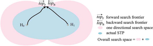
The search space of the naïve SBS method for an AP with one flexible activity is schematically illustrated in Figure 4, in which $to{p}_{\mathrm{F}}+to{p}_{\mathrm{B}}=t_{\mathrm{B}}$ holds in the ideal situation. The two circles are the search spaces of the first two phases (lines 6–9). The search space of the third phase is delineated by excluding the intersected area of the two circles from the blue ellipse. For P2P routing in road networks, the naïve SBS method explores approximately half the space as the unidirectional search does. It implies that the naïve SBS method is generally advantageous over the preprocessing method of Kuijpers and Othman (2009). The search space for STP modeling depends on the value of $t\left({\mathrm{H}}_0,{\mathrm{H}}_1\right)$ in $G$ given fixed $t_{\mathrm{B}}$. If the gap between $t\left({\mathrm{H}}_0,{\mathrm{H}}_1\right)$ and $t_{\mathrm{B}}$ is large, naïve SBS tends to explore less extra space. Particularly, if $t\left({\mathrm{H}}_0,{\mathrm{H}}_1\right)=0$ (${\mathrm{H}}_0$ and ${\mathrm{H}}_1$ are identical), the naïve SBS method is equivalent to applying two unidirectional standard shortest path searches, whose search frontiers are roughly bounded by $\frac{t_{\mathrm{B}}}{2}$. As $t\left({\mathrm{H}}_0,{\mathrm{H}}_1\right)$ becomes larger, the naïve SBS method has better performance than the naïve TBS methods.

Figure 4. Schematic representation of the search space of the naïve SBS method (it is comparable with Figure 1 only when the blue ellipses are drawn on the same scale)

3.2.2. Goal-directed SBS

The naïve SBS method can be extended to goal-directed for further reducing the search space. Potential time expense functions to reach the goals (${\mathrm{H}}_0$ and ${\mathrm{H}}_1$) are required to apply the goal-directed SBS method. Formulated as Equations (12(12) ${\vec{f}}_{{\mathrm{H}}_0{\mathrm{H}}_1}\left(n{|}_s\right)=g_{{\mathrm{H}}_0}\left(n{|}_s\right)+{\vec{h}}_{{\mathrm{H}}_1}\left(n{|}_s\right)$(12) –14(14) $ALT\left(n{|}_s,u{|}_{s^{\prime }}\right)=ALT\left(n,u\right)=max\left\{\left|t\left(n,m\right)-t\left(u,m\right)\right|\right\},m\in M\subset G,\mathrm{\forall }s,s^{\prime }$(14) ), let ${\vec{f}}_{{\mathrm{H}}_0{\mathrm{H}}_1}\left(n{|}_s\right)$ denote a potential activity-travel time from ${\mathrm{H}}_0$ to ${\mathrm{H}}_1$ via an explored frontier node $n{|}_s$, ${\vec{h}}_{{\mathrm{H}}_1}\left(n{|}_s\right)$ an estimated lower bound activity-travel time from $n{|}_s$ to ${\mathrm{H}}_1$, and $ALT\left(\cdot ,\cdot \right)$ the landmark-based lower bound travel time between any two nodes (note that A* method, $e\left(\cdot ,\cdot \right)$, can also be applied here).

(12) ${\vec{f}}_{{\mathrm{H}}_0{\mathrm{H}}_1}\left(n{|}_s\right)=g_{{\mathrm{H}}_0}\left(n{|}_s\right)+{\vec{h}}_{{\mathrm{H}}_1}\left(n{|}_s\right)$(12)

(13) ${\vec{h}}_{{\mathrm{H}}_1}\left(n{|}_s\right)=\sum _{\alpha \in A_s}{d}_{\alpha }+ALT\left(n{|}_s,{\mathrm{H}}_1\right)$(13)

(14) $ALT\left(n{|}_s,u{|}_{s^{\prime }}\right)=ALT\left(n,u\right)=max\left\{\left|t\left(n,m\right)-t\left(u,m\right)\right|\right\},m\in M\subset G,\mathrm{\forall }s,s^{\prime }$(14)

where $m$ is an element from landmark set $M$. As found in Goldberg and Harrelson (2005), the number of selected landmarks $\left|M\right|$ is usually small (e.g. $\left|M\right|=8$) to ensure $e\left(\cdot ,\cdot \right)\le ALT\left(\cdot ,\cdot \right)\le t\left(\cdot ,\cdot \right)$ in real road networks. It means that replacing $e\left(\cdot ,\cdot \right)$ by $ALT\left(\cdot ,\cdot \right)$ is likely to result in a smaller search space. In the opposite search direction, ${\overleftarrow{f}}_{{\mathrm{H}}_0{\mathrm{H}}_1}\left(u{|}_{s^{\prime }}\right)$ and ${\overleftarrow{h}}_{{\mathrm{H}}_1}\left(u{|}_{s^{\prime }}\right)$ are respectively given as Equations (15(15) ${\overleftarrow{f}}_{{\mathrm{H}}_0{\mathrm{H}}_1}\left(n{|}_s\right)=g_{{\mathrm{H}}_1}\left(n{|}_s\right)+{\overleftarrow{h}}_{{\mathrm{H}}_0}\left(n{|}_s\right)$(15) –16(16) ${\overleftarrow{h}}_{{\mathrm{H}}_0}\left(n{|}_s\right)=\sum _{\alpha \in \overline{A_s}}{d}_{\alpha }+ALT\left(n{|}_s,{\mathrm{H}}_0\right)$(16) ) in the reversed $SNK$.

(15) ${\overleftarrow{f}}_{{\mathrm{H}}_0{\mathrm{H}}_1}\left(n{|}_s\right)=g_{{\mathrm{H}}_1}\left(n{|}_s\right)+{\overleftarrow{h}}_{{\mathrm{H}}_0}\left(n{|}_s\right)$(15)

(16) ${\overleftarrow{h}}_{{\mathrm{H}}_0}\left(n{|}_s\right)=\sum _{\alpha \in \overline{A_s}}{d}_{\alpha }+ALT\left(n{|}_s,{\mathrm{H}}_0\right)$(16)

where $\overline{A_s}$ denotes a subset of activities that have been conducted at $s$, $A_s+\overline{A_s}=A$, $\mathrm{\forall }s$. The goal-directed SBS using ALT is referred to as SBS with ALT. Given a link from $n$ to $u$ and a goal ${\mathrm{H}}_1$ in $G$, its transformed link travel time $l\left(n,u\right)-ALT\left({\mathrm{H}}_1,n\right)+ALT\left({\mathrm{H}}_1,u\right)$ is non-negative. It is claimed that ${\vec{h}}_{{\mathrm{H}}_1}\left(n{|}_s\right)$ and ${\overleftarrow{h}}_{{\mathrm{H}}_0}\left(n{|}_s\right)$ in Equations (13(13) ${\vec{h}}_{{\mathrm{H}}_1}\left(n{|}_s\right)=\sum _{\alpha \in A_s}{d}_{\alpha }+ALT\left(n{|}_s,{\mathrm{H}}_1\right)$(13) , 16(16) ${\overleftarrow{h}}_{{\mathrm{H}}_0}\left(n{|}_s\right)=\sum _{\alpha \in \overline{A_s}}{d}_{\alpha }+ALT\left(n{|}_s,{\mathrm{H}}_0\right)$(16) ) are feasible. For example, in the forward search direction, for a link from $n{|}_s$ to $u{|}_{s^{\prime }}$ in $SNK$, the transformed link time expense $l\left(n{|}_s,u{|}_{s{ }^{\mathrm{\prime }}}\right)-{\vec{h}}_{{\mathrm{H}}_1}\left(n{|}_s\right)+{\vec{h}}_{{\mathrm{H}}_1}\left(u{|}_{s{ }^{\mathrm{\prime }}}\right)$ is non-negative. With this property, the forward and backward goal-directed searches are equivalent to standard shortest path searches with reduced link time expenses. In either search direction, any node is only processed (permanently labeled) once. Figure 5 schematically shows the goal-directed SBS process at $n{|}_s$ and $u{|}_{s^{\prime }}$ of both search directions. The right-hand sides of Equations (17(17) $to{p}_{\mathrm{F}}=min{g}_{{\mathrm{H}}_0}\left(n{|}_s\right)\Rightarrow {\overrightarrow{top}}_{\mathrm{F}}=min{g}_{{\mathrm{H}}_0}\left(n{|}_s\right)-{\vec{h}}_{{\mathrm{H}}_1}\left({\mathrm{H}}_0\right)+{\vec{h}}_{{\mathrm{H}}_1}\left(n{|}_s\right)$(17) –18(18) $to{p}_{\mathrm{B}}=min{g}_{{\mathrm{H}}_1}\left(n{|}_s\right)\Rightarrow {\overleftarrow{top}}_{\mathrm{B}}=min{g}_{{\mathrm{H}}_1}\left(n{|}_s\right)-{\overleftarrow{h}}_{{\mathrm{H}}_0}\left({\mathrm{H}}_1\right)+{\overleftarrow{h}}_{{\mathrm{H}}_0}\left(n{|}_s\right)$(18) ) show the modified least time expenses from the source nodes to a common search frontier $n{|}_s$. In that sense, Pseudo-code 2 in Section 3.2.1 can be adapted to find the exact STP.

(17) $to{p}_{\mathrm{F}}=min{g}_{{\mathrm{H}}_0}\left(n{|}_s\right)\Rightarrow {\overrightarrow{top}}_{\mathrm{F}}=min{g}_{{\mathrm{H}}_0}\left(n{|}_s\right)-{\vec{h}}_{{\mathrm{H}}_1}\left({\mathrm{H}}_0\right)+{\vec{h}}_{{\mathrm{H}}_1}\left(n{|}_s\right)$(17)

(18) $to{p}_{\mathrm{B}}=min{g}_{{\mathrm{H}}_1}\left(n{|}_s\right)\Rightarrow {\overleftarrow{top}}_{\mathrm{B}}=min{g}_{{\mathrm{H}}_1}\left(n{|}_s\right)-{\overleftarrow{h}}_{{\mathrm{H}}_0}\left({\mathrm{H}}_1\right)+{\overleftarrow{h}}_{{\mathrm{H}}_0}\left(n{|}_s\right)$(18)

Figure 5. Schematic representation of goal-directed SBS method

The naïve SBS method stops exploring new nodes once $to{p}_{\mathrm{F}}+to{p}_{\mathrm{B}}>t_{\mathrm{B}}$. To derive a similar stopping condition for the goal-directed SBS method, special care is needed to ensure correctness. As both search directions apply transformed link time expenses, the sum of the modified shortest time expenses may not be consistent since ${\vec{h}}_{{\mathrm{H}}_1}\left(n{|}_s\right)+{\overleftarrow{h}}_{{\mathrm{H}}_0}\left(n{|}_s\right)$ may vary with $n{|}_s$. Following the goal-directed methods for P2P routing (Ikeda et al. 1994), this study applies feasible and consistent lower bounds, of which ${\vec{h}}_{{\mathrm{H}}_1}\left(n{|}_s\right)$ and ${\overleftarrow{h}}_{{\mathrm{H}}_0}\left(n{|}_s\right)$ are extended as ${\vec{p}}_{{\mathrm{H}}_1}\left(n{|}_s\right)$ and ${\overleftarrow{p}}_{{\mathrm{H}}_1}\left(n{|}_s\right)$ respectively in Equations (19(19) ${\vec{p}}_{{\mathrm{H}}_1}\left(n{|}_s\right)=\frac{1}{2}\left({\vec{h}}_{{\mathrm{H}}_1}\left(n{|}_s\right)-{\overleftarrow{h}}_{{\mathrm{H}}_0}\left(n{|}_s\right)\right)+\frac{1}{2}{\overleftarrow{h}}_{{\mathrm{H}}_0}\left({\mathrm{H}}_1\right)$(19) –20(20) ${\overleftarrow{p}}_{{\mathrm{H}}_0}\left(n{|}_s\right)=\frac{1}{2}\left({\overleftarrow{h}}_{{\mathrm{H}}_0}\left(n{|}_s\right)-{\vec{h}}_{{\mathrm{H}}_1}\left(n{|}_s\right)\right)+\frac{1}{2}{\vec{h}}_{{\mathrm{H}}_1}\left({\mathrm{H}}_0\right)$(20) ).

(19) ${\vec{p}}_{{\mathrm{H}}_1}\left(n{|}_s\right)=\frac{1}{2}\left({\vec{h}}_{{\mathrm{H}}_1}\left(n{|}_s\right)-{\overleftarrow{h}}_{{\mathrm{H}}_0}\left(n{|}_s\right)\right)+\frac{1}{2}{\overleftarrow{h}}_{{\mathrm{H}}_0}\left({\mathrm{H}}_1\right)$(19)

(20) ${\overleftarrow{p}}_{{\mathrm{H}}_0}\left(n{|}_s\right)=\frac{1}{2}\left({\overleftarrow{h}}_{{\mathrm{H}}_0}\left(n{|}_s\right)-{\vec{h}}_{{\mathrm{H}}_1}\left(n{|}_s\right)\right)+\frac{1}{2}{\vec{h}}_{{\mathrm{H}}_1}\left({\mathrm{H}}_0\right)$(20)

where $0\le {\vec{p}}_{{\mathrm{H}}_1}\left(n{|}_s\right)\le min{g}_{{\mathrm{H}}_1}\left(n{|}_s\right)$, $0\le {\overleftarrow{p}}_{{\mathrm{H}}_0}\left(n{|}_s\right)\le min{g}_{{\mathrm{H}}_0}\left(n{|}_s\right)$, and ${\vec{p}}_{{\mathrm{H}}_1}\left(n{|}_s\right)+{\overleftarrow{p}}_{{\mathrm{H}}_0}\left(n{|}_s\right)={\vec{h}}_{{\mathrm{H}}_1}\left({\mathrm{H}}_0\right)$ hold $\mathrm{\forall }n{|}_s$. Notably, Equations (19(19) ${\vec{p}}_{{\mathrm{H}}_1}\left(n{|}_s\right)=\frac{1}{2}\left({\vec{h}}_{{\mathrm{H}}_1}\left(n{|}_s\right)-{\overleftarrow{h}}_{{\mathrm{H}}_0}\left(n{|}_s\right)\right)+\frac{1}{2}{\overleftarrow{h}}_{{\mathrm{H}}_0}\left({\mathrm{H}}_1\right)$(19) –20(20) ${\overleftarrow{p}}_{{\mathrm{H}}_0}\left(n{|}_s\right)=\frac{1}{2}\left({\overleftarrow{h}}_{{\mathrm{H}}_0}\left(n{|}_s\right)-{\vec{h}}_{{\mathrm{H}}_1}\left(n{|}_s\right)\right)+\frac{1}{2}{\vec{h}}_{{\mathrm{H}}_1}\left({\mathrm{H}}_0\right)$(20) ) often produce worse lower bounds than Equations (13(13) ${\vec{h}}_{{\mathrm{H}}_1}\left(n{|}_s\right)=\sum _{\alpha \in A_s}{d}_{\alpha }+ALT\left(n{|}_s,{\mathrm{H}}_1\right)$(13) , 16(16) ${\overleftarrow{h}}_{{\mathrm{H}}_0}\left(n{|}_s\right)=\sum _{\alpha \in \overline{A_s}}{d}_{\alpha }+ALT\left(n{|}_s,{\mathrm{H}}_0\right)$(16) ). Replacing the updated lower bounds in Equations (17(17) $to{p}_{\mathrm{F}}=min{g}_{{\mathrm{H}}_0}\left(n{|}_s\right)\Rightarrow {\overrightarrow{top}}_{\mathrm{F}}=min{g}_{{\mathrm{H}}_0}\left(n{|}_s\right)-{\vec{h}}_{{\mathrm{H}}_1}\left({\mathrm{H}}_0\right)+{\vec{h}}_{{\mathrm{H}}_1}\left(n{|}_s\right)$(17) –18(18) $to{p}_{\mathrm{B}}=min{g}_{{\mathrm{H}}_1}\left(n{|}_s\right)\Rightarrow {\overleftarrow{top}}_{\mathrm{B}}=min{g}_{{\mathrm{H}}_1}\left(n{|}_s\right)-{\overleftarrow{h}}_{{\mathrm{H}}_0}\left({\mathrm{H}}_1\right)+{\overleftarrow{h}}_{{\mathrm{H}}_0}\left(n{|}_s\right)$(18) ) at a common frontier $n{|}_s$ leads to

(21) ${\overrightarrow{top}}_{\mathrm{F}}+{\overleftarrow{top}}_{\mathrm{B}}=min{g}_{{\mathrm{H}}_0}\left(n{|}_s\right)+min{g}_{{\mathrm{H}}_1}\left(n{|}_s\right)-{\vec{p}}_{{\mathrm{H}}_1}\left({\mathrm{H}}_0\right)-{\overleftarrow{p}}_{{\mathrm{H}}_0}\left({\mathrm{H}}_1\right)$(21)

(22) $=min{g}_{{\mathrm{H}}_0}\left(n{|}_s\right)+min{g}_{{\mathrm{H}}_1}\left(n{|}_s\right)-\frac{1}{2}\left({\vec{h}}_{{\mathrm{H}}_1}\left({\mathrm{H}}_0\right)+{\overleftarrow{h}}_{{\mathrm{H}}_0}\left({\mathrm{H}}_1\right)\right)$(22)

(23) $=min{g}_{{\mathrm{H}}_0}\left(n{|}_s\right)+min{g}_{{\mathrm{H}}_1}\left(n{|}_s\right)-{\vec{h}}_{{\mathrm{H}}_1}\left({\mathrm{H}}_0\right)$(23)

(24) $=min{g}_{{\mathrm{H}}_0}\left(n{|}_s\right)+min{g}_{{\mathrm{H}}_1}\left(n{|}_s\right)-ALT\left({\mathrm{H}}_0,{\mathrm{H}}_1\right)-\sum _{\alpha \in A}{d}_{\alpha }$(24)

where Equations (22(22) $=min{g}_{{\mathrm{H}}_0}\left(n{|}_s\right)+min{g}_{{\mathrm{H}}_1}\left(n{|}_s\right)-\frac{1}{2}\left({\vec{h}}_{{\mathrm{H}}_1}\left({\mathrm{H}}_0\right)+{\overleftarrow{h}}_{{\mathrm{H}}_0}\left({\mathrm{H}}_1\right)\right)$(22) –24(24) $=min{g}_{{\mathrm{H}}_0}\left(n{|}_s\right)+min{g}_{{\mathrm{H}}_1}\left(n{|}_s\right)-ALT\left({\mathrm{H}}_0,{\mathrm{H}}_1\right)-\sum _{\alpha \in A}{d}_{\alpha }$(24) ) are obtained due to Equations (13(13) ${\vec{h}}_{{\mathrm{H}}_1}\left(n{|}_s\right)=\sum _{\alpha \in A_s}{d}_{\alpha }+ALT\left(n{|}_s,{\mathrm{H}}_1\right)$(13) , 14(14) $ALT\left(n{|}_s,u{|}_{s^{\prime }}\right)=ALT\left(n,u\right)=max\left\{\left|t\left(n,m\right)-t\left(u,m\right)\right|\right\},m\in M\subset G,\mathrm{\forall }s,s^{\prime }$(14) , 16(16) ${\overleftarrow{h}}_{{\mathrm{H}}_0}\left(n{|}_s\right)=\sum _{\alpha \in \overline{A_s}}{d}_{\alpha }+ALT\left(n{|}_s,{\mathrm{H}}_0\right)$(16) ). $ALT\left({\mathrm{H}}_0,{\mathrm{H}}_1\right)=0$ if ${\mathrm{H}}_0$ and ${\mathrm{H}}_1$ in $G$ are identical. Equation (24)(24) $=min{g}_{{\mathrm{H}}_0}\left(n{|}_s\right)+min{g}_{{\mathrm{H}}_1}\left(n{|}_s\right)-ALT\left({\mathrm{H}}_0,{\mathrm{H}}_1\right)-\sum _{\alpha \in A}{d}_{\alpha }$(24) has two implications with the transformed link time expenses. First, the shortest activity-travel times of all paths from ${\mathrm{H}}_0$ to ${\mathrm{H}}_1$ via $\mathrm{\forall }n{|}_s$ are reduced by $ALT\left({\mathrm{H}}_0,{\mathrm{H}}_1\right)+\sum _{\alpha \in A}{d}_{\alpha }$, which is constant given the AP. Second, the condition of stopping exploring new nodes in the goal-directed SBS method becomes Equation (25)(25) ${\overrightarrow{top}}_{\mathrm{F}}+{\overleftarrow{top}}_{\mathrm{B}}>t_{\mathrm{B}}-ALT\left({\mathrm{H}}_0,{\mathrm{H}}_1\right)-\sum _{\alpha \in A}{d}_{\alpha }$(25) .

(25) ${\overrightarrow{top}}_{\mathrm{F}}+{\overleftarrow{top}}_{\mathrm{B}}>t_{\mathrm{B}}-ALT\left({\mathrm{H}}_0,{\mathrm{H}}_1\right)-\sum _{\alpha \in A}{d}_{\alpha }$(25)

Similar to the naïve SBS, the goal-directed SBS goes through three phases and has one watershed point drawn by Equation (25)(25) ${\overrightarrow{top}}_{\mathrm{F}}+{\overleftarrow{top}}_{\mathrm{B}}>t_{\mathrm{B}}-ALT\left({\mathrm{H}}_0,{\mathrm{H}}_1\right)-\sum _{\alpha \in A}{d}_{\alpha }$(25) , after which no new nodes will be explored in either search direction. The goal-directed SBS method necessitates three adjustments in Pseudo-code 2: (i) to modify link time expenses when extending the frontiers in lines 7 and 12; (ii) to replace the inequality in line 5 by Equation (25)(25) ${\overrightarrow{top}}_{\mathrm{F}}+{\overleftarrow{top}}_{\mathrm{B}}>t_{\mathrm{B}}-ALT\left({\mathrm{H}}_0,{\mathrm{H}}_1\right)-\sum _{\alpha \in A}{d}_{\alpha }$(25) ; and (iii) to implement the replacement of Equations (17(17) $to{p}_{\mathrm{F}}=min{g}_{{\mathrm{H}}_0}\left(n{|}_s\right)\Rightarrow {\overrightarrow{top}}_{\mathrm{F}}=min{g}_{{\mathrm{H}}_0}\left(n{|}_s\right)-{\vec{h}}_{{\mathrm{H}}_1}\left({\mathrm{H}}_0\right)+{\vec{h}}_{{\mathrm{H}}_1}\left(n{|}_s\right)$(17) –18(18) $to{p}_{\mathrm{B}}=min{g}_{{\mathrm{H}}_1}\left(n{|}_s\right)\Rightarrow {\overleftarrow{top}}_{\mathrm{B}}=min{g}_{{\mathrm{H}}_1}\left(n{|}_s\right)-{\overleftarrow{h}}_{{\mathrm{H}}_0}\left({\mathrm{H}}_1\right)+{\overleftarrow{h}}_{{\mathrm{H}}_0}\left(n{|}_s\right)$(18) ). The correctness of the goal-directed SBS method is concluded as Corollary 3.

Corollary 3: The exact STP can be constructed by the goal-directed SBS method in $SNK$.

Proof. With the feasible and consistent bidirectional lower bounds, the goal-directed SBS is equivalent to the naïve SBS with modified link time expenses. According to Lemma 2, the goal-directed SBS method constructs the exact STP.

Compared with the naïve SBS method, the goal-directed SBS implicitly incorporates temporal feasibility checking through inequalities $min{g}_{{\mathrm{H}}_0}\left(n{|}_s\right)+{\vec{p}}_{{\mathrm{H}}_1}\left(n{|}_s\right)\le t_{\mathrm{B}}$ and $min{g}_{{\mathrm{H}}_1}\left(n{|}_s\right)+{\overleftarrow{p}}_{{\mathrm{H}}_0}\left(n{|}_s\right)\le t_{\mathrm{B}}$. These conditions can largely exclude nodes that are not in the STP but explored by the naïve SBS method. When ${\vec{p}}_{{\mathrm{H}}_1}\left(n{|}_s\right)={\overleftarrow{p}}_{{\mathrm{H}}_0}\left(n{|}_s\right)=0,\mathrm{\forall }n{|}_s$, the naïve SBS method is considered a special case of the goal-directed SBS.

Compared with the goal-directed TBS method, the goal-directed SBS method explores larger space before the watershed point arises because ${\vec{p}}_{{\mathrm{H}}_1}\left(n{|}_s\right)$ is worse than ${\vec{h}}_{{\mathrm{H}}_1}\left(n{|}_s\right)$ in most cases. After crossing the watershed point, the forward search space of the goal-directed TBS continues expanding and is bounded by Equation (9)(9) $min{g}_{{\mathrm{H}}_0}\left(n{|}_s\right)+\sum _{\alpha \in A_s}{d}_{\alpha }+e\left(n{|}_s,{\mathrm{H}}_1\right)\le t_{\mathrm{B}}$(9) or $min{g}_{{\mathrm{H}}_0}\left(n{|}_s\right)+{\vec{h}}_{{\mathrm{H}}_1}\left(n{|}_s\right)\le t_{\mathrm{B}}$ (see the pink skewed ellipse in Figure 1 for example); however, the goal-directed SBS method starts to search and check the temporal feasibility only within the actual PPA. Figure 6 schematically illustrates the search space of the goal-directed SBS method for one flexible activity. Using the same syntax, the blue ellipse represents the actual PPA in Figure 6. At the top and bottom intersections, ${\overrightarrow{top}}_{\mathrm{F}}+{\overleftarrow{top}}_{\mathrm{B}}$ is equal to $t_{\mathrm{B}}-{\vec{h}}_{{\mathrm{H}}_1}\left({\mathrm{H}}_0\right)$. The two skewed pink ellipses (partly covered by the blue one) constitute the search space of the first two phases, and the blue elliptical area excluding the intersected area of the two pink ellipses is the search space of the third phase. Nonetheless, it is not direct to judge if one method is certainly more effective than another given the presence of multiple determinants. When there is an ideal feasible lower bound (i.e., ${\vec{h}}_{{\mathrm{H}}_1}\left(n{|}_s\right)$ approximates $min{g}_{{\mathrm{H}}_1}\left(n{|}_s\right)$), the goal-directed TBS is supposed to explore less space and be more computationally efficient since ${\vec{p}}_{{\mathrm{H}}_1}\left(n{|}_s\right)$ is usually worse than ${\vec{h}}_{{\mathrm{H}}_1}\left(n{|}_s\right)$ and needs more processing time. When ${\vec{h}}_{{\mathrm{H}}_1}\left(n{|}_s\right)$ is not good enough (i.e., ${\vec{h}}_{{\mathrm{H}}_1}\left(n{|}_s\right)$ is close to zero), the goal-directed SBS method resembles the naive one; thus, when $min{g}_{{\mathrm{H}}_0}\left({\mathrm{H}}_1\right)$ approaches $t_{\mathrm{B}}$ (i.e., the time budget is tight), the goal-directed SBS method becomes more effective.

Figure 6. Schematic representation of the search space of the goal-directed SBS method (it is comparable with Figures 1 and 3 only when the blue ellipses are drawn on the same scale)

Taken together, it is therefore claimed that all the bidirectional search methods can pinpoint the exact STP and PPA (illustrated with a small example in Part 2 of the supplementary document). A flowchart incorporating both TBS and SBS methods is shown in Figure 7. The following general remarks are made. First, provided with good lower bounds of activity-travel times, the goal-directed TBS and SBS methods are more effective than the naïve counterparts in terms of search space. When the time budget is tight, the goal-directed formalism leads to computational efficiency without loss of optimality. If the time budget is slack, goal-directed TBS and SBS lose the advantage of smaller search space but incur the disadvantage of more processing time.

Figure 7. Flowchart of the TBS and SBS methods

Second, different potential functions would work in goal-directed search methods. In the context of daily APs, the time budget is usually tight due to chained time window constraints. If there are fixed activities in an AP, the lower bounds can be improved by considering the compulsive trips to the fixed locations if the activity states permit. For example, if fixed activity $\alpha$ at node $u{|}_s$ is not conducted yet, the adjusted lower bound ${\vec{h}}_{u_{\mathrm{s}}}\left(n{|}_s\right)+{\vec{h}}_{{\mathrm{H}}_1}\left(u{|}_s\right)$ is better than ${\vec{h}}_{{\mathrm{H}}_1}\left(n{|}_s\right)$.

Third, the approximation method in Liao (2019) does not necessarily explore less space than goal-directed TBS and SBS in that the unidirectional goal-directed (forward) search is applied twice for calculating the lower and upper bounds of ${\vec{f}}_{{\mathrm{H}}_0{\mathrm{H}}_1}(n{|}_s)$. In addition, the approximation method applies buffers and heuristic partial ATPs to generate bound values, which is also computationally demanding. These limitations are remedied in the bidirectional search scheme.

Fourth, in terms of running time complexity, the class of goal-directed methods is evaluated differently depending on the formation of the potential functions. As the goal-directed searches are equivalent to the standard shortest path searches with feasible lower bounds, the running time complexity is no worse than $O\left(2^{\left|A\right|}\cdot \left|N\right|\cdot log\left|N\right|\right)$ in $SNK$ for all aforementioned methods. Similar to evaluating the performances of speedup techniques for P2P routing, the search space is a major indicator. One point worth noting is that the SBS methods are run in parallel and naturally support parallel computing.

4. Experimental tests

This section compares and illustrates the bidirectional search methods in large networks. First of all, to show the accuracy, the proposed methods are compared with the approximation method in Liao (2019) considering the same AP in the same transport network. Second, to show the computational efficiency, the proposed methods are compared with the methods in Kuijpers and Othman (2009) and Chen et al. (2016) in grid networks. Sensitivity analyses are conducted to analyze the impacts of time budget. For landmark selection, Goldberg and Harrelson (2005) found that a small number of random landmarks produce satisfactory speedups and scattered landmarks can achieve even better results. For the applications of the ALT method in the GIS field, it is recommended to select a few (e.g. ranged from 6 to 12) scattered landmarks at the borders of the transport networks. Computational efficiency is tested in large grid networks with randomly generated anchor points. All methods are executed with C++ on a PC using one core of Intel® CPU 3.40 GHz, 8 G RAM.

4.1. Illustration of accuracy compared with the approximation method in Liao (2019)

The study area concerns the Eindhoven-Helmond corridor (the Netherlands) in Figure 8. The AP consists of three activities: work, shopping, and leisure with minimum durations of 480, 10, and 50 min respectively (i.e., $\left|A\right|=3$). For the sake of illustration, some settings are simplified from the actual situation. The detailed settings are as follows.

Figure 8. Eindhoven-Helmond corridor (scale: 1:150,000)

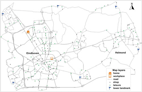
(1) Home and workplace are fixed locations. The time windows for conducting all out-of-home activities and work are [8:30, 18:30] and [9:00, 17:00] respectively, which means $t_0=8:30$ and $t_{\mathrm{B}}=600$ min. There are 100 location alternatives for shopping (in black dots) and 100 for leisure (in green dots). The service time windows for shopping and leisure are [8:00, 19:00] and [11:00, 21:00] respectively.

(2) The road network includes 4,828 nodes and 12,208 directed links. Roads are classified into three types, i.e. <local, local priority, regional>. Maximum bike and car speed limits on these road types are set as <18, 18, 24> and <40, 60, 80> in km/h respectively. Suppose that it takes two minutes for one episode of picking-up or parking a car.

(3) Six landmarks ($\left|M\right|=6$) are randomly selected near the border (flags) for calculating $ALT\left(\cdot ,\cdot \right)$ in Equation (14)(14) $ALT\left(n{|}_s,u{|}_{s^{\prime }}\right)=ALT\left(n,u\right)=max\left\{\left|t\left(n,m\right)-t\left(u,m\right)\right|\right\},m\in M\subset G,\mathrm{\forall }s,s^{\prime }$(14) , of which $t\left(\cdot ,m\right)$ $\mathrm{\forall }m$ is preprocessed once by running six times of one-to-all shortest path procedure.

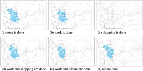
With the above setting, the unimodal multi-state supernetwork includes six activity states, 28,968 nodes, and 73,650 links due to a strict time window constraint, i.e. work prior to leisure. All the bidirectional search methods discussed in Section 3 can pinpoint the exact state-dependent PPAs shown in Figure 9 (by car) and Figure 10 (by bike). Amongst, the naïve SBS method needs the most computation times (0.02 s), which is three times faster than the approximation method (0.06 s) in Liao (2019). The state-dependent STPs can be obtained by attaching time ranges in the 3-D space according to line 16 of Pseudo-code 2. Each state-dependent PPA covers the location opportunities to implement the remainder activities. The PPAs vary with activity states and the sizes of PPAs by car are larger than those by bike. Particularly, the PPA in Figure 10(c) is empty, implying that it is impossible to complete the AP by bike if shopping is conducted first.

Figure 9. Exact activity state-dependent PPAs (in blue) by car

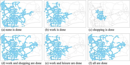
Figure 10. Exact activity state-dependent PPAs (in blue) by bike

Table 3 shows the numbers of accessible shops and leisure locations at the relevant states. As seen, the numbers of accessible locations delineated by the approximate and exact methods differ. Due to the use of buffer areas and heuristic rules, the approximation method slightly underestimated the PPAs when traveling by car and overestimated the PPAs when traveling by bike. It implies that the contours of the exact state-dependent PPAs do not completely fall inside the rings of the approximate lower and upper PPA bounds produced by the method of Liao (2019). The comparison demonstrates that the bidirectional search scheme is advantageous in terms of accuracy.

Table 3. Numbers of accessible locations (lower – upper bound in Liao (2019)/exact)

Activity state	Using car		Using bike
	Shop	Leisure	Shop	Leisure
None is done	63–64/77	69–72/77	31–33/25	30–31/26
Work is done	53–59/62	55–61/67	23–29/24	21–26/23
Shopping is done	n/a	11–17/23	n/a	0–0/0
Work and shopping are done	n/a	81–82/87	n/a	26–31/26
Work and leisure are done	56–61/62	n/a	28–33/21	n/a

(n/a: not applicable as the activity is done at the state; the exact numbers of locations are in bold.)

4.2. Illustration of computation efficiency in grid networks

4.2.1. One activity

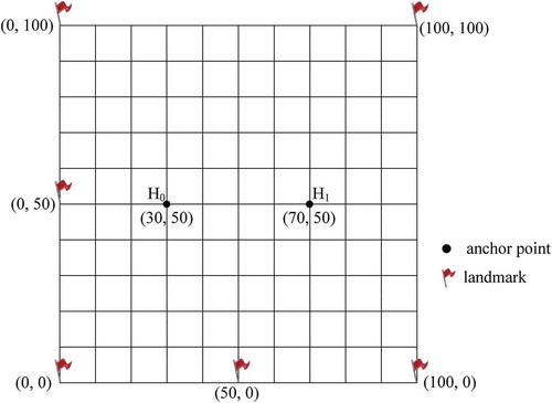
In this example, a grid network (Figure 11 – one line every 10 units) is a geographically square area with 101 by 101 (or 10,201) nodes and 40,400 directed travel links of an equal length (1 km). All links are located either horizontally or vertically and have travel times (link travel speeds) randomly generated from three possibilities, i.e., 2 min (30 km/h), 1.2 min (50 km/h), and 0.75 min (80 km/h). The left-bottom and right-top corners correspond to coordinators $\left(0,0\right)$ and $\left(100,100\right)$ respectively. This AP specifies $t_0=0$, $t_1=120$ min, two anchors ${\mathrm{H}}_0$ at coordinator ($30,50)$ and ${\mathrm{H}}_1$ at $\left(70,50\right)$, and a flexible activity $\alpha$ ($d_{\alpha }=$40 min) that can be conducted at any node in the network. For the goal-directed search using A*, the maximum speed is 80 km/h and the distance between nodes is Euclidean based on coordinators. For using ALT, six coordinators at the border, namely, $\left(0,0\right)$, $\left(0,50\right)$ $\left(50,0\right)$ $\left(100,0\right)$, $\left(0,100\right)$, and $\left(100,100\right)$, are selected as the landmarks.

Figure 11. Grid network for one flexible activity

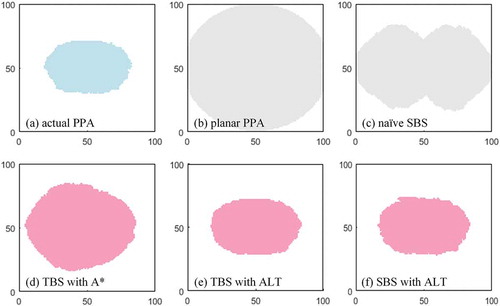
Based on the setup, the search spaces of different methods are shown in Figure 12. Subgraphs (a-b) show the actual and planar PPAs covering 2,100 and 8,171 nodes respectively. Likewise, the STP can be obtained by attaching time ranges in the 3-D space over the actual PPA. Similar to other prism shapes, the central areas of the PPA have wider time ranges than other areas. Subgraphs (c-f) correspond to the search spaces of the naïve SBS, TBS with A* (Chen et al. 2016), TBS with ALT, and SBS with ALT, which cover 5,391, 4,236, 2,465, and 2,575 nodes respectively. Their search areas should additionally encompass the actual PPA for checking the temporal feasibility. Recall that the preprocessing method of Kuijpers and Othman (2009) searches the planar PPA twice. TBS and SBS with ALT explore less than 2.5% extra nodes that do not belong to the actual PPA, while naïve SBS and TBS with A* explore up to 150% and 100% redundant nodes beyond the actual PPA. The computation times are positively correlated with the search space. It takes around 0.002 sec by searching twice in the planar PPA, 0.001 sec by the naïve SBS (subgraph (c)) and TBS with A* (subgraph (d)), and less than 0.001 sec by the TBS and SBS with ALT (subgraphs (e) and (f)). In this example, the results indicate the outperformance of goal-directed methods over the standard method and ALT over A*.

Figure 12. Search spaces of different methods

To test the influence of time budge on the search space, sensitivity analysis is carried out on the distance between the two anchor points. Keeping the y-coordinators of ${\mathrm{H}}_0$ and ${\mathrm{H}}_1$ unchanged, the x-coordinator pair is changed from 25–75 to 50–50 with common differences of 5 and −5 respectively. The set of x-coordinator pairs of H₀ and H₁ to be examined equals {25-75, 30–70, 35–65, 40–60, 45–55, 50–50}. The extra nodes explored by different methods beyond the actual PPA in percentages are shown in Figure 13. 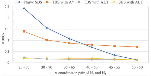It is observed that TBS and SBS with ALT explore significantly less space when the time budget is tight (i.e., the distance between ${\mathrm{H}}_0$ and ${\mathrm{H}}_1$ is large) and the naïve SBS tends to exhibit substantially improved performance with increasing time budget (i.e., the distance between ${\mathrm{H}}_0$ and ${\mathrm{H}}_1$ is small). As for computation time, TBS with ALT slightly outperforms SBS with ALT because the former only involves half the processing time of the latter. Without preprocessing, nonetheless, the naïve SBS excels other methods when the time budget is slack.

Figure 13. Extra nodes explored beyond the actual PPA of different methods

4.2.2. Three activities

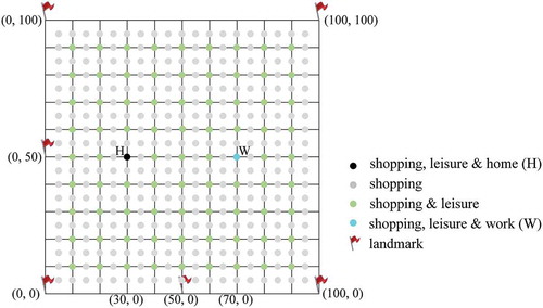
In the same grid network, this AP consists of three activities: work, shopping, and leisure with minimum durations of 480, 10, and 50 min respectively. Suppose the locations are at the following coordinators (Figure 14): home (H) at (30, 50), work (W) at (70, 50), shopping at $\left\{\left(5\times i,5\times j\right)|0<i,j<20,i,j\in {\mathbb{N}}^{+}\right\}$, and leisure at $\left\{\left(10\times i,10\times j\right)|0<i,j<10,i,j\in {\mathbb{N}}^{+}\right\}$. The shopping and leisure activities have 361 and 81 alternative locations with service time windows [8:00, 18:00] and [9:00, 20:00], respectively; the work activity has a time window [9:00, 17:00]. This AP specifies conducting the three activities and returning home between 7:45 and 19:00 (i.e., $t_{\mathrm{B}}=675$ min). With the setup, a unimodal $SNK$ is first constructed, which has 6 states due to the time window constraints (i.e., work prior to leisure), resulting in 61,206 nodes and 243,286 links.

Figure 14. Grid network for one AP of three activities with flexible activity sequences

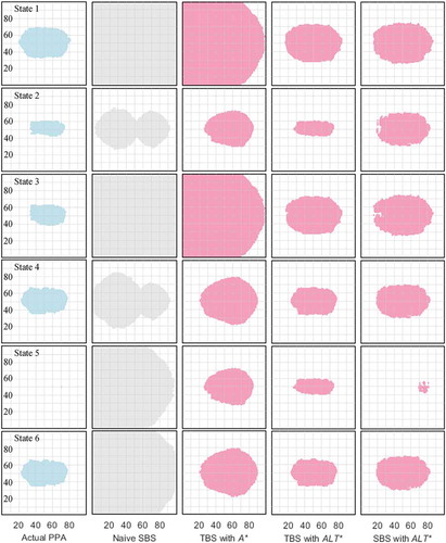
Figure 15 shows the actual activity state-dependent PPAs (1st column) and search spaces of different methods (2nd–5th columns) labeled at the bottom. Due to space limitations, only the results of four method variants of interest are shown. Each row represents one activity state. States 1–6, respectively, refer to activity states ‘none is done’, ‘work is done’, ‘shopping is done’, ‘work and shopping are done’, ‘work and leisure are done’, and ‘all activities are done’. The same syntaxes are used for the colored areas. The actual activity state-dependent PPAs vary due to time window constraints and activity chains. Specifically, the PPA at state 5 consists of only one node since shopping can only be conducted at coordinator (70, 50), where work and leisure are also conducted. The search spaces also vary with different methods. The planar PPA covers the entire network. The naïve SBS method cancels out a large number of infeasible areas at states 2 and 4. The TBS with A* removes many infeasible nodes at states 5 and 6. Utilizing preprocessing sufficiently, TBS and SBS with ALT* explore less space, where ALT* stands for the consideration of a trip to the fixed work location (W) in the ALT method at states 1 and 3. The search spaces of the SBS with ALT* are partly discontinuous due to temporal feasibility checks, which do not exclude locations in the actual state-dependent PPAs.

Figure 15. State-dependent PPAs and search spaces of different methods

Table 4 displays the numbers of nodes explored and computation times. The results show that TBS with ALT* has the best performance and SBS with ALT* ranks second. It is worth noting that TBS and SBS with ALT* still explore more than 64% extra nodes, signifying the room to derive better lower bounds of activity-travel times. Sensitivity analysis is also run to test the impacts of time budget. Keeping the y-coordinators of H and W unchanged, the x-coordinator pair is changed from 25–75 to 50–50 with common differences of 5 and −5 respectively. The extra nodes explored by different methods are shown in Figure 16. It indicates that an AP with more activities overall requires more extra search space than a single flexible activity because time window constraints and activity chains cause redundancy. For the same reason, SBS with ALT* does not achieve the expected effects, while TBS with ALT* has stable performances.

Figure 16. Extra nodes explored beyond the actual PPA of different methods

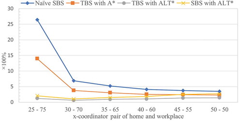
Table 4. Numbers of nodes explored and computation times

	Actual PPA	Naïve SBS	TBS with A*	TBS with ALT*	SBS with ALT*
Number of nodes explored	5,883	46,335	28,111	9,625	12,061
Extra nodes beyond actual PPA	n/a	687%	379%	64%	105%
Computation time (sec)	n/a	0.008	0.007	0.004	0.006

4.2.3. Computational efficiency

As formulated in Section 3, $\left|N\right|$ (the number of nodes in $G$) is the main determinant of running time complexity given that $\left|A\right|$ (the number of activities) is usually small. To show the computational efficiency, the search methods are run for the above two representative APs in grid networks of four different sizes, i.e., 101 by 101, 251 by 251, 501 by 501, and 1001 by 1001. To make the comparisons intuitive, the link lengths are decreased proportionally to 0.4 km, 0.2 km, and 0.1 km in the latter three grid networks, while the random link travel speeds remain unchanged. Moreover, the physical locations for landmarks, shopping, and leisure are roughly the same as specified in Section 4.2 for the second AP. 1000 random ${\mathrm{H}}_0$-${\mathrm{H}}_1$ anchor pairs for the first AP and 1000 random home locations for the second AP are respectively generated in each grid network. The computation times of different methods in the four grid networks are shown in Table 5, of which invalid pairs resulting in empty PPAs are removed without replacement. Combing with the above sensitive analyses, the results show that the naïve SBS is computationally efficient despite larger search spaces for the first AP and that TBS with ALT* is more efficient than others for the second AP.

Table 5. Computation time in second for 1000 random pairs (the least times are in bold)

1st AP					2nd AP
Size Method	101^2	251^2	501^2	1001^2	Size Method	101^2	251^2	501^2	1001^2
Naïve SBS	0.481	3.77	20.24	93.32	Naïve SBS	6.48	45.93	219.9	995.4
TBS with A*	0.634	4.88	28.06	117.5	TBS with A*	5.29	32.78	143.7	602.8
TBS with ALT	0.497	3.73	27.49	94.16	TBS with ALT*	3.06	18.41	85.66	355.7
SBS with ALT	0.627	4.69	20.73	114.0	SBS with ALT*	5.34	34.07	173.2	816.2

The results comply with the remarks in Section 3 that goal-directed search methods, in general, explore fewer nodes, especially when the time budget is tight. For the first AP, naïve SBS uses slightly shorter computation times than TBS with ALT in three cases because it needs the least preprocessing time. For the second AP, the plausible large time budget results in a planar PPA covering the entire supernetwork; however, due to the chained time windows, the time budget is compressed so that the naïve SBS loses the advantage. Surprisingly, SBS with ALT* does not achieve the efficiency as expected for P2P routing as it does not have an absolute lead in reducing search space but requires longer preprocessing times. The fourth grid network has more than one million nodes and four million links, and the corresponding multi-state supernetwork has more than 6 million nodes and 24 million links. This supernetwork size is large enough to accommodate the majority of APs in urban areas. Regarding the preprocessing time in the ALT method, as only a few landmarks are selected, it is trivial to run one-to-all shortest path algorithms from the landmarks compared with large-scale analyses. Storing the precalculated shortest travel times requires some overhead time, but it is only linear in the network size, meaning a marginal preprocessing time. Taken together, it takes only 0.92 sec to preprocess the 1001 by 1001 grid network. Thus, the above-mentioned bidirectional search methods, especially naïve SBS and TBS with ALT⁽*⁾, are feasible for large-scale prism-based analyses.

5. Conclusions and discussions of future research

STP modeling for APs, as opposed to single flexible activities, is a challenging research topic. This paper proposed a bidirectional search scheme to construct the exact STP of an individual’s AP in a multi-state supernetwork, which structurally represents the action space and path set for conducting the activities. It is proved that the TBS methods that have been developed for constructing trip-based STPs are also effective. It is also found that the suggested SBS methods are capable of sufficiently utilizing the results of the forward and backward search directions. Compared with the unidirectional search method in Liao (2019), all the proposed search methods can delineate the exact STP. Amongst, TBS with ALT⁽*⁾ on average has the best performance in terms of space exploration and computation time, and the naïve SBS achieves a surprising outperformance when the time budget is slack.

Nevertheless, a few issues regarding the model extensions and applications are worth further investigation. First, as STP modeling highlights mobility constraints, besides the temporal dimension, it is important to incorporate other mobility-related constraints such as interpersonal interactions and monetary costs to improve model realism. Second, the search methods should be extended to accommodate supply dynamics related to temporal variations and stochasticity in the multimodal transport networks. Such extensions should be viable given the existence of corresponding P2P routing algorithms. To that effect, more dedicated search adjustments should be made. Third, in addition to space–time accessibility measures, the findings of this study have vast applications in urban and transport studies. For example, the method can be embedded in travel demand analysis models for location choice set formation; in combination with revealed mobility data, the method can be applied to measure quality-of-life indices such as social exclusion and equity to access the built environment. Fourth, the current study is theoretic-oriented and it is interesting to examine the relevance of the theoretical outcomes with human mobility boundaries delimited by geodata-based empirical research. For the above issues, it should be noted that the multi-state supernetworks remain a powerful representation of the action space and path set. These issues will be addressed in future work.

Acknowledgments

The author is indebted to Angela B.J.L. in the challenging times in 2020.

Data and codes availability statement

The data and codes that support the findings of this study are available in figshare.com with the identifier(s) at the link https://doi.org/10.6084/m9.figshare.13108094.v2.

Disclosure statement

No potential conflict of interest was reported by the author.

Additional information

Notes on contributors

Feixiong Liao

Feixiong Liao is an assistant professor at the Urban Planning and Transportation Group of Eindhoven University of Technology (the Netherlands). His research interests include activity-based modeling, accessibility analysis, discrete choice modeling, and supernetwork modeling for applications in urban planning and transportation research.

References

- Bast, H., et al. 2016. Route planning in transportation networks. Route planning in transportation networks. In: L. Kliemann & P. Sanders editors. Algorithm engineering, Cham.: Springer, 19–80.
- Chen, B.Y., et al. 2013. Reliable space–time prisms under travel time uncertainty. Annals of the Association of American Geographers, 103 (6), 1502–1521. doi:https://doi.org/10.1080/00045608.2013.834236.
- Chen, B.Y., et al. 2017. Measuring place-based accessibility under travel time uncertainty. International Journal of Geographical Information Science, 31 (4), 783–804. doi:https://doi.org/10.1080/13658816.2016.1238919.
- Chen, H.P., et al., 2016. Efficient geo-computational algorithms for constructing space–time prisms in road networks. International Journal of Geo-Information, 5 (11), 1–16.
- Chen, X. and Kwan, M.-P., 2012. Choice set formation with multiple flexible activities under space–time constraints. International Journal of Geographical Information Science, 26 (5), 941–961. doi:https://doi.org/10.1080/13658816.2011.624520.
- Doran, J., 1967. An approach to automatic problem-solving. Machine Intelligence, 1, 105–127.
- Goldberg, A.V. and Harrelson, C., 2005. Computing the shortest path: A* search meets graph theory. In: Proceedings of 16th Annual ACM–SIAM Symposium on Discrete Algorithms, 23–25 January 2005 Vancouver, Canada: Society for Industrial and Applied Mathematics, 156–165.
- Hägerstrand, T., 1970. What about people in regional science? Papers in Regional Science Association, 24, 7–21.
- Hu, Y., Janowicz, K., and Chen, Y., 2016. Task-oriented information value measurement based on space–time prisms. International Journal of Geographical Information Science, 30 (6), 1228–1249.
- Ikeda, T., et al., 1994. A fast algorithm for finding better routes by AI search techniques. In: Proceedings of the Vehicle Navigation and Information Systems Conference, Yokohama, Japan: ACM Press, 291–296.
- Kang, J.E. and Chen, A., 2016. Constructing the feasible space–time region of the household activity pattern problem. Transportmetrica A, 12, 591–611.
- Kuijpers, B., Miller, H.J., and Othman, W., 2017. Kinetic prisms: incorporating acceleration limits into space–time prisms. International Journal of Geographical Information Science, 31, 2164–2194.
- Kuijpers, B. and Othman, W., 2009. Modeling uncertainty of moving objects on road networks via space–time prisms. International Journal of Geographical Information Science, 23, 1095–1117.
- Kwan, M.-P. and Hong, X.D., 1998. Network-based constraints-oriented choice set formation using GIS. Journal of Geographical Systems, 5, 139–162.
- Lenntorp, B., 1976. Path in space–time environments: a time-geographic study of the movement possibilities of individuals. In: B. Lenntorp editor. Lund studies in geography B. Lund: CWK Gleerup, 1–150.
- Liao, F., 2016. Modeling duration choice in space–time multi-state supernetworks for individual activity-travel scheduling. Transportation Research Part C, 69, 16–35.
- Liao, F., 2019. Space–time prism bounds of activity programs: A goal-directed search in multi-state supernetworks. International Journal of Geographical Information Science, 33, 900–921.
- Liao, F., Arentze, T.A., and Timmermans, H.J.P., 2010. Supernetwork approach for multimodal and multiactivity travel planning. Transportation Research Record, 2175, 38–46.
- Liao, F., Arentze, T.A., and Timmermans, H.J.P., 2011. Constructing personalized transportation networks in multi-state supernetworks: a heuristic approach. International Journal of Geographical Information Science, 25, 1885–1903.
- Liao, F., Arentze, T.A., and Timmermans, H.J.P., 2013. Incorporating space–time constraints and activity-travel time profiles in a multi-state supernetwork approach to individual activity-travel scheduling. Transportation Research Part B, 55, 41–58.
- Liao, F., Rasouli, S., and Timmermans, H.J.P., 2014. Incorporating activity-travel time uncertainty and stochastic space–time prisms in multistate supernetworks for activity-travel scheduling. International Journal of Geographical Information Science, 28, 928–945.
- Mahmoudi, M., et al. 2019. Accessibility with time and resource constraints: computing hyper-prisms for sustainable transportation planning. Computers, Environment and Urban Systems, 73, 171–183.
- Miller, H.J., 1991. Modelling accessibility using space–time prism concepts within geographical information systems. International Journal of Geographical Information Systems, 5, 287–301.
- Miller, H.J., 2017. Time geography and space–time prism. In: D. Richardson, N. Castree, M. F. Goodchild, A. Kobayashi, W. Liu, & R. A. Marston editors. The international encyclopedia of geography. Sussex: Wiley, 1–19.
- Neutens, T., 2015. Accessibility, equity and health care: review and research directions for transport geographers. Journal of Transport Geography, 43, 14–27.
- Neutens, T., Schwanen, T., and Witlox, F., 2011. The prism of everyday life: towards a new research agenda for time geography. Transport Reviews, 31, 25–47.
- Song, Y., et al. 2017. Green accessibility: estimating the environmental costs of network-time prisms for sustainable transportation planning. Journal of Transport Geography, 64, 109–119.