Qualitative spatial reasoning with uncertain evidence using Markov logic networks

Abstract

Probabilistic logics combine the ability to reason about complex scenes, with a rigorous approach to uncertainty. This paper explores the construction of probabilistic spatial logics through the combination of established qualitative spatial calculi together with Markov logic networks (MLNs). Qualitative spatial calculi provide the basis for automated representation and reasoning with complex spatial scenes; MLNs provide a rigorous basis for handling uncertainty and driving probabilistic inference. Our approach focuses specifically on the combination of an uncertain knowledge base with a certain spatial reasoning rule-base. The experiments explore how uncertain knowledge propagates through certain qualitative spatial inferences, using the specific example of reasoning with cardinal directions. The results provide a template for probabilistic qualitative spatial reasoning more generally, with applications to a wide range of common scenarios for situational awareness and automated reasoning under uncertainty.

Keywords:

• Markov logic network
• qualitative spatial reasoning
• uncertainty
• cardinal direction calculus

1. Introduction

Qualitative spatial reasoning (QSR) is an established body of techniques in knowledge representation and reasoning (KR), concerned with the discrete, imprecise and non-numerical properties of space and time. In general, there are three main motivations for the use of qualitative reasoning (Galton 2000, Duckham 2008, Wolter and Wallgrün 2013):

• qualities supervene (i.e. can be derived from) quantities (e.g. bearing of 274° is ‘left‘);

• qualities are conceptually simpler than quantities (e.g. ‘hot‘ versus 32.18 °C); and,

• qualities usually correspond to discontinuities that are salient to humans (e.g. ‘left‘ versus ‘right‘, ‘in front‘ versus ‘behind‘).

Today, qualitative spatial calculi exist for reasoning about a rich variety of spatial relations, including location, topology, cardinal and relative directions, orientation and visibility (Ligozat 2013, Dylla et al. 2018). A range of practical tools for QSR have been developed, including the SparQ toolbox (Dylla et al. 2006, Wallgrün et al. 2006, Wolter and Wallgrün 2013) and QSRlib (Gatsoulis et al. 2016).

While qualitative spatial calculi capture the inherent imprecision of human spatial concepts (such as ‘left‘ and ‘right‘, ‘north‘ and ‘south‘, ‘inside‘ and ‘outside‘), they do not offer a ready mechanism to reason about wider sources of uncertainty in spatial scenes. In the simple taxonomy proposed by Worboys and Clementini (2001), uncertainty results from imperfection in data; imprecision is a type of imperfection connected with lack of detail in data; and inaccuracy, synonymous with error, is an orthogonal type of imperfection connected with a lack of correctness in data. Although many other types of uncertainty have been discussed in the spatial literature (e.g. Chrisman 1991, Guptill and Morrison 1995, Fisher 1999), most can be described in terms of imprecision and inaccuracy. Ambiguity, for example, is a special case of imprecision. Vagueness – an important area of study in its own right (Keefe and Smith 1996) – can be regarded as a form of boundary imprecision (Worboys and Clementini 2001) (and discussed further below).

This paper is specifically concerned with spatial reasoning under uncertainty where:

1. spatial data may be imprecise (e.g. ‘northwest‘ and ‘southeast‘ do not provide detail about the exact direction);

2. spatial inferences may be imprecise (e.g. if A is northwest of B and B is northwest of C, then we can be certain that A is northwest of C; but if B is northeast of D, then we may be certain only that A is northeast, northwest or north of D); and

3. imprecise spatial data may also be subject to error (inaccuracy), for example, where we must acknowledge the possibility that evidence indicating that A is northwest of B may in actuality be incorrect.

Our approach is founded on the significant body of work in QSR that comprehensively addresses those cases where (1) and (2) above hold. Incorporating inaccuracy of evidence ((3) above), however, is a significant challenge that relatively few spatial reasoning techniques have yet addressed. This is discussed further below. In this paper, we explore the adoption of Markov logic networks (MLNs) as a mechanism to extend QSR ((1) and (2) above) with handling of such ‘soft‘ evidence ((3) above). MLNs combine first-order-logic (FOL) with probabilistic graphical models (Richardson and Domingos 2006). FOL formulae handle the complexity of reasoning, while probabilistic graphical models provide a rigorous framework for handling the propagation of uncertainty through the reasoning process (Sabek 2019).

Hence, our approach can handle not only imprecision in spatial reasoning, but also inaccuracy in data through the medium of probability. For example, we aim to answer questions of the form: if there is a 70% likelihood that point A is to the south of point B and a 40% likelihood that point B is to the northeast of point C, then what is the probability distribution over all possible cardinal directions from point A to point C? Accordingly, the key contributions of this paper are as follows:

• We provide a blueprint for augmenting qualitative spatial logics with the capacity to handle uncertain evidence (i.e. inputs) using MLNs. We include a working example using a simplified direction calculus to demonstrate the implementation of QSR with MLNs. We show how this prototype can be easily applied to other spatial logics.

• We explore empirically the effectiveness of an MLN-based QSR engine to respond to queries based on uncertain evidence. Specifically, we explore the example of reasoning with uncertain evidence using the cardinal direction calculus (CDC) to answer queries of the form: ‘What is the most likely direction of object A from location B?‘

• We outline a roadmap for implementing a generic framework for probabilistic QSR, based on qualitative spatial calculi and MLNs, and highlight the key research challenges facing that initiative.

The organization of the remainder of the paper is as follows. Section 2 summarizes the related literature associated with QSR and reasoning with uncertainty. Our proposed framework for spatial reasoning with MLNs is set out in Section 3, including a minimal working example using a direction calculus. Section 4 introduces the implementation of a common variant of the CDC within an MLN as an extended example. Section 5 then explores empirically the results of using MLNs together with the CDC as the basis for probabilistic and QSR with uncertain evidence. In particular, we explore three different types of uncertainty in evidence with increasing levels of sophistication: soft evidence of qualitative spatial relations; soft evidence across conceptual neighborhoods; and soft evidence in the presence of inconsistency. Finally, we conclude this article in Section 6.

2. Related work

2.1. Qualitative spatial reasoning

One of the most influential early examples of qualitative reasoning is Allen’s interval calculus (Allen 1983, Freksa 1992). Building on a single, primitive ‘meets‘ relation between two temporal intervals, Allen’s interval calculus constructs 13 distinct qualitative relations (equals, before, after, during, contains, as well as meets, finishes, starts, overlaps and their converses). In common with most qualitative calculi that followed, this basic set of relations is jointly exhaustive pairwise disjoint (JEPD): the relationship between any two temporal intervals is described by one and only one qualitative interval relation in the set, which in union describes all the possible relations between the intervals.

In the same vein, another well-known approach to qualitative spatial logic is the region connection calculus (RCC) of Randell et al. (1992). RCC is founded on binary connection relations between regions, where $\mathsf{C}(A,B)$ is a primitive dyadic relation denoting region A is connected to region B. RCC-5 (Bennett 1994) constructs five binary base relations from region connection: inside (proper part $\mathsf{PP}$) and contains (proper part inverse $\mathsf{PPi}$), equals ($\mathsf{EQ}$), disjoint (disjoint region $\mathsf{DR}$) and overlap (partial overlap $\mathsf{PO}$). RCC-8 further refines these relations, distinguishing boundary cases: touches ($\mathsf{EC}$, externally connected, where region boundaries only touch) and disconnected ($\mathsf{DC}$, disconnected), as a refinement of RCC-5’s disjoint region $\mathsf{DR}$ relation; and covered by, its converse covers ($\mathsf{TPP}$ and $\mathsf{TPPi}$ tangential proper part/inverse, where regions are contained except at a tangential shared boundary), and properly contained/contains ($\mathsf{NTPP}$ and $\mathsf{NTPPi}$ non-tangential proper part/inverse), as refinements of RCC-5’s proper part $\mathsf{PP}$ and proper part inverse $\mathsf{PPi}$ (Li and Ying 2003). The topological relations between two regions and their corresponding classifications in RCC-5 and RCC-8 are shown in Table 1.

A range of qualitative representations also exist for describing direction relations. Frank (1992) defines eight cardinal direction relations based on two schemes: point-based conical and region-based projective directions. Extensions to the approach by Balbiani et al. (1999) and Goyal and Egenhofer (2001) provide a further mechanism for reasoning about qualitative direction relations between two regions in the plane.

Freksa (2005) extends the projective approach by describing qualitative direction of a particular landmark (relatum) relative to the intrinsic orientation of an observer (origin). Freksa’s ‘double-cross‘ calculus distinguishes 15 base relations in such cases, for example, discerning apart straight ahead past the landmark; straight behind the observer; and straight between observer and landmark (Scivos and Nebel 2001). Other oriented direction calculi include the dipole calculus, based on pairs of oriented straight line segments (Schlieder 1995); the OPRA2 calculus, using oriented points (Mossakowski and Moratz 2012, 2015); and the CYCORD calculus, based on pure directions/orientations not anchored at locations (Isli and Cohn 1998, Moratz 2017).

Building on ideas in direction calculi, the qualitative trajectory calculus (QTC) provides a qualitative description of movement and trajectories. QTC is based on three aspects of movement: the movement of each point with respect to the position of the other at time t and the relative (qualitative) speeds of the objects (Van de Weghe et al. 2005, 2006).

In addition to region, direction and trajectory relations, many other qualitative spatial representations have been developed, including for qualitative size and distance, shape, and vagueness and indeterminacy (Cohn and Hazarika 2001, Cohn and Renz 2008). In most cases, qualitative spatial calculi adopt a constraint-based representation, with constraints specified over a set of base relations (Renz and Nebel 2001, Cohn and Renz 2008). For example, $\mathsf{DR}(A,B)\vee \mathsf{PO}(A,B)$ expresses the RCC-5 constraint that region A and B are either disjoint or overlap.

The basis of logical inference in QSR is then the (weak) composition of relations. For example, in RCC-5 for any three regions A, B, C, if we know $\mathsf{PPi}(A,B)$ (A contains B) and $\mathsf{PPi}(B,C)$ (B contains C), then we can infer the new knowledge that $\mathsf{PPi}(A,C)$ (A also contains C). Unfortunately, not all inferences are as discerning. For example, if instead $\mathsf{PO}(B,C)$ (B and C overlap), then, we can infer that either A contains or overlaps C (i.e. $\mathsf{PPi}(A,C)\vee \mathsf{PO}(A,C)$). For a fuller discussion of the weak composition operation in QSR, see Renz and Ligozat (2005). Together with a converse operation (e.g. converse of $\mathsf{PP}(A,B)$ is $\mathsf{PPi}(B,A)$), the composition operation can then form the basis for a relation algebra (Tarski 1941).

2.2. Uncertain spatial reasoning

Qualitative spatial reasoning enables us to represent the inherently imprecise nature of many types of spatial knowledge. For example, RCC-5 enables us to represent and reason about relations between regions, such as when one region is inside another, without needing to commit to precise quantitative location or geometry. As such, it has been contended that QSR is especially congruent with human spatial cognition, sometimes described as ‘cognitively plausible‘ (Freksa 1991).

While tolerant to imprecision, most qualitative spatial calculi do not provide mechanisms for reasoning about other forms of uncertainty, commonly found in human spatial cognition (Ragni et al. 2016). RCC-5 and RCC-8, for example, assume that the boundaries of regions are precisely defined, often not true in real-world scenarios. In everyday communication, we may frequently refer to regions with imprecise boundaries. In Cohn and Gotts (1996a) and Cohn et al. (1997), the authors presented the ‘egg-yolk‘ calculus, extending RCC-5 regions with a zone of boundary indeterminacy around a certain, core region. Taking a different approach, Petry et al. (2005) and Schockaert et al. (2009) applied fuzzy sets to regions and RCC relations. In Petry et al. (2005), the authors applied an extended version of Allen’s algorithm (Allen 1983) to compute the local consistency of fuzzy networks with RCC-8 relations. Schockaert et al. (2009) investigated the satisfiability, entailment checking and inconsistency repairing for such fuzzy RCC relations.

In a related approach to that taken in this paper, Girlea and Amir (2015) developed a possible worlds semantics for probabilistic RCC, modeling the joint probability distribution over spatial relations using Markov random fields (MRFs). The approach results in the definition of a more expressive RCC, where one can distinguish the most probable relation from among all the possible relations between two regions. An advantage of this approach is that it yields clearly defined syntax and semantics for RCC. In comparison, our work starts from a purely symbolic perspective based on using MLNs (indeed, this approach is also suggested by Girlea and Amir (2015) as an alternative to their approach). As a consequence, our approach can be directly applied to a range of different qualitative spatial logics, and is not specific to reasoning with RCC, as we show below. Further, our approach provides a richer model of the uncertainty associated with evidence. In practice, this means our model is able to deal with contradictory and mutually inconsistent evidence, which is common in practice for reasoning with data from multiple different human and physics-based sources.

Many other approaches have been proposed for spatial reasoning under uncertainty. In early work, Loerch and Guesgen (1997) explore the combination of quadtrees with fuzzy methods to reason about the proximity of uncertain regions. Closer to our approach is the work of Emrich et al. (2012) that is interested in queries concerning presence or absence of dynamic objects in a given region of space over a specified time interval. The positions of the dynamic objects are assumed to be uncertain and changing over time. Markov chains are used to model positional uncertainties in order to support efficient querying over multiple epochs. A similar problem is addressed in Banerjee et al. (2014) where the authors are interested in uncertain trajectories of moving objects. A historical database of trajectories is used to overcome the limitations of Markovian motion models, and a Gibbs Sampler to estimate the most likely trajectory. Finally, Schultz et al. (2016) use constraint logic programming to allow spatial reasoning tasks to be represented as a numerical optimization problem with soft constraints.

2.3. Spatial reasoning and MLNs

This work is not the first to explore the use of MLNs for qualitative reasoning. For example, Snidaro et al. (2015) combine MLNs with Allen’s interval algebra (Allen 1983) to reason with incomplete data and contextual knowledge about the relationship between events. The approach is tested on two maritime situational awareness scenarios: rendezvous events at sea and meetings between potentially hazardous combinations of cargo ships in port. In a similar vein, Alevizos and Artikis (2018) propose pattern Markov chains (PMCs) to represent and reason about maritime events and forecast likely future events. These two approaches use contextual knowledge, such as temporal and spatial adjacency, to support reasoning about specific maritime scenarios. Our work extends such approaches to the richer spatial context provided by qualitative spatial logics, including reasoning with direction or topological relations.

In other work by Sabek et al. (2019), MLNs are applied to the problem of generic and scalable spatial data analysis. The focus of the ‘Flash‘ framework in Sabek et al. (2019) is on learning qualitative spatial knowledge from copious quantities of big spatial data, as the basis for subsequent automated qualitative reasoning. The flexibility of the Flash framework has been demonstrated in Sabek et al. (2019) through three specific applications: predicting the presence of bird species based on spatial data about known bird locations; inferring qualitative knowledge about level of safety, based on spatial data about crime incidents; and inferring qualitative knowledge about land use change based on historical spatial data about land cover.

Likewise, Nguyen (2019) emphasizes the potential of using MLNs to support reasoning about complex, real-world situations by learning from abundant but uncertain big data. The objective of Nguyen (2019) is ‘off-domain reasoning‘: automatically inferring semantic relationships (such as taxonomy or mereology) between concepts already encoded in a semantic knowledge base, and unfamiliar terms encountered in situational awareness applications. In common with our work, both the Flash framework and Nguyen (2019) aim at generic applicability. However, the focus of Sabek et al. (2019), Sabek (2019) and Nguyen (2019) is on learning new and uncertain inference rules from big data. In contrast, our work begins with pre-existing, certain qualitative spatial logics, and instead focuses on the impact of uncertain evidence upon inference.

Our approach is perhaps closest in aims to Nguyen and Mellor (2020), who propose combining fuzzy sets with qualitative spatiotemporal knowledge using MLNs, extending the maritime situational awareness applications presented in Nguyen (2019). However, Nguyen and Mellor (2020) approach is particularly concerned with the related but distinct issue of vague evidence. Vagueness concerns the existence of boundary cases (Cohn and Gotts 1996b, Keefe and Smith 1996). Many common qualitative spatial relations, such as ‘nearness‘, are also vague (Duckham and Worboys 2001, Worboys 2001). For example, while some ships may be unambiguously ‘near‘ a port – and others unambiguously ‘not near‘ a port – there will typically be instances of ships for which it is indeterminate whether they are or are not ‘near‘ a port. Although vagueness is undoubtedly an enduring challenge for reasoning about geography (Varzi 2001), this current paper focuses specifically on crisp, rather than vague, spatial objects and relations.

In conclusion, in contrast to previous research, this paper is about reasoning with established qualitative spatial logics while exploring the propagation of uncertain evidence through the QSR process, rather than learning special rules from data.

3. Spatial reasoning with MLNs

3.1. Preliminaries

Markov logic networks are introduced and explored in a wealth of literature on the subject, in particular, the seminal work Richardson and Domingos (2006) and Domingos et al. (2008), to which the reader is referred for a detailed formal treatment. The focus of this paper is not on the theoretical development of MLNs; rather its aim is to apply them to a particular class of spatial reasoning problems. For this reason, we briefly recap the foundations of MLNs as the core of the inference engine we use.

A MLN is a first-order knowledge base. More specifically, an MLN is a set of pairs (F_i, w_i), where F_i is a formulae in first order logic (FOL) and w_i is a corresponding weight associated with that formula. Weights represent a level of confidence in that formula. Each formula is constructed from constants, variables, functions and predicates:

• Constants represent object instances in the domain of interest, e.g. City of Melbourne, RMIT University.

• Functions relate objects to one another, e.g. $\mathit{CapitalOf}(\mathit{Australia})=\mathit{Canberra}.$

• Predicates capture the properties of objects, e.g. $\mathit{adjacent}(\mathit{Australia},\mathit{Austria})=\mathit{false}.$

FOL formulae can be recursively combined using connectives (negation, $\neg ;$ conjunction, $\wedge ;$ disjunction, $\vee ;$ logical equivalence, $\iff ;$ and implication, $\Rightarrow$) and quantifiers (universal quantification, $\forall ,$ and existential quantification, $\exists$). Variables are also used to construct formulae that range over objects of specific types (e.g. city, university). A predicate expression that contains no variables is called a ground predicate. Similarly, a formula containing no variables is a ground formula. The process of assigning constant terms to each variable is referred as grounding. A possible world is an assignment of truth values to all possible ground atoms (Richardson and Domingos 2006).

To support reasoning, the structure of an MLN knowledge base is encoded as a MRF. An MRF, also called a Markov network, models the joint distribution of a set of random variables $X=\{X_1,\dots ,X_n\}.$ An MRF can be represented as an undirected graph, where each variable maps to a node in the graph and a neighborhood structure $N_i(i=1,2,\dots ,n)$ is specified – a neighborhood is assigned to each node.

There is a great deal of flexibility in the definition of the neighborhood structure, and it can be designed to suit specific purposes. In an MLN, an associated MRF can be constructed with nodes being groundings of the predicates that appear as atomic components the formulae F_i in the knowledge base. Two nodes are adjacent (neighbors) in the graph when two ground predicates appear in the same ground formula. A set of nodes in the MRF in which every node is a neighbor of every other node is termed a clique. Therefore, each ground formula from an MLN maps to a clique in the associated MRF.

Each node in the MRF can now be assigned a binary truth value: 1 if the grounding of that predicate is true and 0 otherwise. Standard formulae in MRFs lead to the following probability distribution on all possible worlds (associated with the Hammersley–Clifford theorem, Hammersley and Clifford 1971, again we refer to Richardson and Domingos 2006 for details): (1) $$P(X=x)=\frac{1}{Z}\exp \hspace{0.17em}(\sum _i{w}_i{n}_i(x))$$(1) where $n_i(x)$ is the number of true groundings of F_i; and Z denotes a normalizing factor: $$Z=\sum _x\sum _i{w}_i{n}_i(x).$$

The next step in reasoning with MLNs is to find the most probable state of predicates given some evidence of a world x. One example of such a situation would involve knowing the values of some variables, or the truth values of some formulae F_i. The most probable world, given the evidence, maximizes the conditional probability. Based on how the joint probability distribution was defined in the MLN, the most probable world y is calculated as below: (2) $$\underset{y}{\text{arg} \max }P(y|x)={\underset{y}{\text{arg} \max }}_{}\frac{1}{Z_x}\exp \hspace{0.17em}(\sum _i{w}_i{n}_i(x,y))$$(2) where $n_i(x,y)$ is the number of true groundings of F_i consistent with x and y and w_i is the weight associated with F_i.

3.2. Inference under uncertainty

Using MLNs, we can reason from uncertain evidence. The literature with respect to Bayesian and Markov networks often distinguishes a particular type of uncertainty, called soft evidence, as the probability that an assignment of the value x₁ to the random variable X₁ is in actuality true. We denote the set of observed variables as X_E and the set of unobserved variable as X_U so that $X_E\cap X_U=\varnothing$ and $X_E\cup X_U=X,$ where X is the entire set of variables. Soft evidence is then a constraint on the probability distribution over X_E. Specifically, soft evidence of a variable X_i with binary probability distribution $〈p_i,1-p_i〉$ states that the posterior probability for X_i = true is p_i.

MC-SAT-PC (Jain and Beetz 2010) is an inference method for MLN that is able to consume soft evidence and propagate the uncertainty to the probability of a query. MC-SAT-PC defines a Markov chain Monte Carlo (MCMC) sampling process for possible worlds with probability distribution satisfying the MLN as well as the evidence. The normalization term of Equation (2)(2) $$\underset{y}{\text{arg} \max }P(y|x)={\underset{y}{\text{arg} \max }}_{}\frac{1}{Z_x}\exp \hspace{0.17em}(\sum _i{w}_i{n}_i(x,y))$$(2) is, naturally, adjusted to Z_x by restricting consideration on to those worlds consistent with the evidence. Since we will often adopt a maximum a posteriori (MAP) approach, where only the most probable world is of interest (not its actual probability), the normalization term can be ignored.

In practice, a query is usually related to a specific set of predicates. To determine the conditional probability of a predicate, the probability of all possible worlds that satisfy the predicate need to be accumulated. The possibility of a world x is proportional to the exponentiated sum of weights of formulae satisfied by x, as shown in Equation (1)(1) $$P(X=x)=\frac{1}{Z}\exp \hspace{0.17em}(\sum _i{w}_i{n}_i(x))$$(1) . With $\hspace{0.17em}\exp \hspace{0.17em}(\sum _i{w}_i{n}_i(x))=:w(x),$ the probability of a ground formula F₁ given another ground formula F₂ as evidence can be calculated, as follows: (3) $$\begin{array}{cc}P(F_1|F_2)\hfill & =\frac{P(F_1,F_2)}{P(F_2)}\hfill \\ \hfill & =\frac{\sum _{x\models F_1\wedge F_2}w(x)}{\sum _{x\models F_2}w(x)}\hfill \end{array}$$(3) where $x\models F_1\wedge F_2$ considers all the worlds where both ground formulae F₁ and F₂ are true.

The calculation of an exact probability (as in Equation (3)(3) $$\begin{array}{cc}P(F_1|F_2)\hfill & =\frac{P(F_1,F_2)}{P(F_2)}\hfill \\ \hfill & =\frac{\sum _{x\models F_1\wedge F_2}w(x)}{\sum _{x\models F_2}w(x)}\hfill \end{array}$$(3) ) involves iterating through all possible worlds. As a result, exact inference using MLNs is intractable in general, and not possible for most realistic use cases. In practice, statistical sampling is usually adopted by MLN inference algorithms to enable efficient calculation of an approximate value to the joint probability distribution instead. The MC-SAT-PC algorithm allows uniform sampling from possible worlds that satisfy a set of ground predicates, where the set is updated at each iteration of the algorithm. The likelihood that a ground formula (i.e. rule) or predicate (i.e. evidence) is selected for the sample at any iteration is related to the weights associated with each the formula or predicate. The larger the weight associated with a piece of evidence or a rule, the more likely the corresponding evidence is selected at any given iteration. Certain evidence or formulae can be represented using infinitely large weights. Any certain evidence or rules will always be selected in every sampled possible world.

3.3. Probabilistic qualitative spatial reasoning

A significant body of existing work in MLNs has focused on using machine learning in data-rich applications to automatically infer weights for FOL formulae (Wick et al. 2010), such as in maritime applications (Snidaro et al. 2015) or genetic analysis (Sakhanenko and Galas 2010, Brouard et al. 2013). In contrast, qualitative spatial calculi provide a ready spatial rule base for certain inferences. Taking again the example of RCC-5 (Randell et al. 1992), assuming region A is truly inside region B, and region B is truly inside region C, then it must necessarily follow that region A is truly inside region C. Given such a certain spatial rule base, uncertainty arises through the evidence used to derive inferences (e.g. whether in fact region A is truly inside region B, and whether region B is truly inside region C). Knowledge of this soft evidence will exhibit correlations and dependencies across different relations and predicates.

We are now ready to set out our approach to probabilistic QSR. We represent uncertain qualitative spatial knowledge as a knowledge base containing:

1. a (certain) rule-base derived from constraint-based qualitative spatial calculi defining qualitative spatial relations, their composition, and converses as FOL rules; and

2. a (soft) evidence-base, containing groundings of those relations, with weights indicating associated uncertainty, that describe a specific spatial scene.

This knowledge base can then be used to construct an MLN in the standard way, as described earlier. Note that MLNs in general may have weights attached both to evidence and to rules in the rule-base. However, in our application of MLNs to spatial reasoning, weights are applied to evidence only. Rules in the rule-base are assumed to be certain (i.e. infinitely large weight) as indicated above (1). The following subsection provides a concrete but highly simplified example to illustrate.

3.4. Simplified direction calculus as an MLN

To demonstrate how qualitative spatial calculi can be implemented as an MLN, we introduce a very simple direction calculus we call the east–west calculus. Our east–west calculus defines just three JEPD binary relations between points in the plane:

• $\mathsf{E}(A,B)$ indicates point A lies to the east of point B;

• $\mathsf{W}(A,B)$ indicates point A lies to the west of point B; or

• $\mathsf{T}(A,B)$ indicates point A lies somewhere on the north–south axis passing through point B.

In order to translate this constraint-based representation into compact FOL rules, we define the ternary predicate $at,$ where $at(A,B,r)$ indicates r(A, B), where $r\in \{\mathsf{E},\mathsf{W},\mathsf{T}\}.$ Following the syntax of Alchemy (one of the first implementations of MLNs, with variables denoted by lower case, and constants by capital letters (Richardson et al. 2007)), the first-order logical rule-base capturing this calculus is given in Table 2. Formulae F₁ and F₂ capture the converse operation and formula F₃ captures the composition operation on relations.

The MLN rule-base in Table 2 defines a template for building a MRF. Figure 1 shows the MRF resulting from this MLN grounded with constants A and B. There are, in total, 12 nodes in the MRF as possible ground predicates (listed in the first column of Table 3). In Figure 1, there exists an edge between every two nodes when the two corresponding ground predicates appear in the same ground formula. For instance, we have a ground formula $at(A,B,\mathsf{E})\iff at(B,A,\mathsf{W})$ when assigning constants A, B to variables a, b, respectively. Ground predicates $at(A,B,\mathsf{E})$ and $at(B,A,\mathsf{W})$ are directly connected with an edge in the MRF.

Next, a possible world is defined by states (truth values) assigned to all the nodes in the MRF. To demonstrate how the equations can be applied for inference, we compare three specific possible worlds W_a, W_b and W_c. Table 3 shows the truth values of all the ground predicates in the three possible worlds. For instance, the entry corresponding to $at(A,B,\mathsf{E})$ (i.e. point A is to the east of point B) is true in world W_a, indicated with a value of 1. The same predicate is false in world W_b, indicated with a 0.

Based on the truth values of ground predicates, the truth values of ground formulae can also be computed using the semantics of whether a ground formula is satisfied in a specific possible world. For example, Table 4 shows all groundings for formula F₁, and their truth values in worlds W_a, W_b and W_c. As shown in Table 4, world W_a agrees with all four groundings of formula F₁. It also agrees with all four groundings of formula F₂; and all eight groundings of F₃. World W_b similarly agrees with all groundings of all formulae. W_c violates some of the formulae and has fewer true ground formulae (e.g. in W_c, $at(A,B,\mathsf{W})$ is false but $at(B,A,\mathsf{E})$ is true, hence $at(A,B,\mathsf{E})\iff at(B,A,\mathsf{W})$ and $at(B,A,\mathsf{E})\iff at(A,B,\mathsf{W})$ are false).

In the absence of any evidence, and in a universe where all rules are certain, W_a and W_b are both possible, while W_c is not possible. However, an uncertain universe, containing evidence or rules that may be ‘soft‘, changes this binary perspective of possibility, making some worlds more likely than others, and – crucially for logical reasoning – making some worlds now possible, which would have otherwise been impossible. In an MLN, such possibilities are activated by assigning weights to both evidence and formulae. Thus, possible worlds full of uncertainties and inconsistencies can still be compared and ranked using probabilities.

In an MLN, evidence can be introduced through probabilities attached to nodes (i.e. ground predicates) in the MRF in Figure 1. For example, the ground predicate $at(A,B,\mathsf{E})$ (line 4) in Table 3 could be weighted to indicate evidence that $at(A,B,\mathsf{E})$ has a 70% chance of being true.

Once this soft evidence is observed, posterior probabilities (Equation (2)(2) $$\underset{y}{\text{arg} \max }P(y|x)={\underset{y}{\text{arg} \max }}_{}\frac{1}{Z_x}\exp \hspace{0.17em}(\sum _i{w}_i{n}_i(x,y))$$(2) ) can be used to drive inference about the probability distribution across the different possible worlds. Based on Equation (1)(1) $$P(X=x)=\frac{1}{Z}\exp \hspace{0.17em}(\sum _i{w}_i{n}_i(x))$$(1) , the probability of a particular world is an increasing function of $\sum _i{w}_i{n}_i(x).$ The MLN inference engine enables observed evidence probabilities to be propagated throughout the MRF. This in turn enables the computation of the associated probabilities for any nodes across different worlds, and indeed the most probable world.

For instance, introducing the evidence that $at(A,B,\mathsf{E})$ has a 70% chance of being true means $at(A,B,\mathsf{E})\iff at(B,A,\mathsf{W})$ will be counted in $n_1(W_a)$ – the number of groundings of formula F₁ that are satisfied in the possible world W_a (see Section 3.1), but not in W_b. In this case, world W_b becomes less consistent with the evidence for $at(A,B,\mathsf{E})$ than world W_a and W_a emerges as the most probable world.

3.5. Scalability of MLN inference

An issue facing any MLN is that the number of possible worlds increases exponentially with the size of the ground Markov network. The size of the ground network, in turn, is determined by the number of constants (nodes) as well as the coincidence of predicates in formulas (edges). In the context of using MLNs for spatial reasoning, this translates into increased computational demands as spatial logics become more complicated (i.e. connecting more predicates in more formulae) and when there are more objects in the scene. The procedure for exact probability computation, introduced in Section 3.4, involves enumerating all possible worlds and consequently is, in general, intractable for spatial reasoning.

The issue of scalability of MLN inference is widely recognized as one of the limitations of MLNs for practical application to large reasoning problems. As a result, significant research effort from across AI has begun to be focused on scalable MLN inference. In general, this effort has focused on two key steps in MLNs:

1. grounding: generating a ground Markov network given a set of MLN formulas and constants; and

2. searching: searching for solutions that maximize the weights.

For each step, various techniques are being explored as the basis for increasingly efficient and scalable inference. For instance, one of the first MLN implementations – Alchemy – spent 96% of its execution time on grounding (Niu et al. 2011). A proposed technique termed ‘lifted inference‘ holds the possibility that a fully grounded network may not be needed for inference (Sarkhel et al. 2014). During the searching phase, traversing each individual possible world quickly becomes intractable as the size of the Markov network increases. In response, a wide variety of sampling techniques, such as MaxWalkSAT (Kautz et al. 1997) and MC-SAT (Poon and Domingos 2006), have been applied to efficiently approximate query results.

Accordingly, the experiments presented in this paper (Section 5) use inference based on MC-SAT-PC (Jain and Beetz 2010), which is a variant of MC-SAT designed for inference with soft evidence. However, beyond acknowledging the need for such sampling to ensure inference with MLNs is tractable, this paper does not explore further the computational characteristics and scalability of QSR using MLNs. Such computational issues are undoubtedly important to understand in exploring the practical application of the techniques developed in this paper. However, exploring such issues is itself a significant undertaking, since it depends not only on the chosen spatial logics and the specific reasoning scenarios, but also on the specific sampling techniques and software implementations used. Hence, a systematic computational analysis of the approach is set aside as a major focus of future work. The scope of this present paper is restricted to developing the foundational techniques for QSR with uncertain evidence using MLNs.

Finally, while MLN inference is a computationally challenging task, we note that future computational advances in this area are made more likely by the large community of AI and statistics researchers already working on the development of such general-purpose probabilistic reasoning tools. Translating the problem of probabilistic spatial reasoning into the context of MLN inference ensures that any such future research advances will also directly benefit the spatial reasoning community.

4. Implementation

The east–west calculus described above is a simplified version of a widely studied qualitative spatial calculus: the CDC (Frank 1992, Goyal and Egenhofer 2001, Skiadopoulos and Koubarakis 2004, Cohn et al. 2014). A number of other variants of the CDC are in the literature (Skiadopoulos and Koubarakis 2004), including direction relations between extended regions and with arbitrarily fine granularity of directions. In our experiments in the following section, we opt for a simple CDC variant introduced in Frank (1992). The CDC partitions the plane relative to a reference point or relatum into nine labeled parts: $\mathsf{N},\mathsf{S},\mathsf{E},\mathsf{W},\mathsf{NE},\mathsf{NW},\mathsf{SE},\mathsf{SW}$ and $\mathsf{I}$ (which translates into the identity relation in a point-based calculus). The spatial relation between the relatum and the referent or locatum (object to be located) is then described by naming that part of the partition in which the referent lies.

Figure 2 illustrates the CDC using a specific spatial scene with direction relations between four spatial objects (points), O₁, O₂, F₁, F₂. The spatial partition includes four (topologically open, semi-bounded) regions induced from the main two directional axis N–S and E–W intersecting at the reference point. However, note that this figure is purely schematic to aid in understanding the qualitative representation and its associated logical inferences. The figure should not be taken to imply that cardinal directions represented either along lines or in regions have any different weighting, importance or geometric structure in the qualitative spatial calculus used to represent and reason with relations between the spatial objects (see Frank 1992, Goyal and Egenhofer 2001, Skiadopoulos and Koubarakis 2004).

For example, with reference to point O₁ (relatum) in Figure 2, we can observe the direction relations to the other three objects (locata) as: $\mathsf{SE}(O_2,O_1),\mathsf{S}(F_1,O_1)$ and $\mathsf{NE}(F_2,O_1).$ Then, $\mathsf{SE}(O_2,O_1)$ can be read informally as ‘object O₂ (locatum) is south-east of object O₁ (relatum)‘. Reasoning using the nine direction relations can then be achieved through valid composition and converse operations. For example, $\mathsf{SE}(O_2,O_1)\iff \mathsf{NW}(O_1,O_2)$ (converse) and $\mathsf{S}(F_1,O_1)\wedge \mathsf{SE}(O_2,F_1)\Rightarrow \mathsf{SE}(O_2,O_1)$ (composition).

Full composition and converse tables can be found in Frank (1992), Skiadopoulos and Koubarakis (2004). Rather than a constraint-based representation, the MLN requires translation into a FOL rule base, as discussed earlier. Table 5, formulae C₁–C₂₆, gives the complete rule base for our CDC variant. The rule base translates the standard constraint-based representation into a first-order logical form using a ternary relation $\mathit{dir}(b,a,r)$ where $r\in \{\mathsf{NE},\mathsf{NW},\mathsf{SE},\mathsf{SW},\mathsf{N},\mathsf{S},\mathsf{E},\mathsf{W},\mathsf{I}\}$ (e.g. $\mathit{dir}(O_2,O_1,\mathsf{SE})$ from Figure 2). Using a ternary relation over multiple binary relations (used in early examples) is more convenient in the probabilistic context because it ensures the probabilities of different relations between a pair of objects adds up to 1.

Each of the rules in Table 5 encodes different constraints. For example, formula C₁ encodes the constraint that a point is always in direction relation $\mathsf{I}$ with itself (e.g. $\mathit{dir}(A,A,\mathsf{I})$). Formulae C₂–C₅ encode the constraints connected with opposite directions (e.g. $\mathit{dir}(B,A,\mathsf{N})$ implies $\mathit{dir}(A,B,\mathsf{S})$). Formulae C₆–C₈ allow us to infer the composition of two relations in the same direction. For example, given the knowledge (premises) $\mathit{dir}(B,A,\mathsf{NE})$ and $\mathit{dir}(C,B,\mathsf{NE}),$ formula C₈ allows us to infer that $\mathit{dir}(C,A,\mathsf{NE}).$

Note that – unlike the original composition table – of the total 8 × 8 = 64 possible composition rules between the eight cardinal directions, Table 5 contains only 21 such composition rule instances (formulae C₆–C₂₆). This is because some composition rules may be inferred from others already in the rule base. For example, with reference to Figure 2, we would wish to be able to conclude $\mathit{dir}(O_2,O_1,\mathsf{SE})$ from the premises $\mathit{dir}(F_1,O_1,\mathsf{S})$ and $\mathit{dir}(O_2,F_1,\mathsf{SE}).$ Although there exists no single explicit rule in the rule base such that $\mathit{dir}(b,a,\mathsf{S})\wedge \mathit{dir}(c,b,\mathsf{SE})\Rightarrow \mathit{dir}(c,a,\mathsf{SE}),$ this rule is implied by the composition rule in formula C₉ combined with the converse rules in formula C₂ and C₄.

The rule-base in Table 5 was implemented within an MLN using the PyMLN/ProbCog software framework (Tenorth et al. 2010). Although there is a variety of free and open source software implementations of MLNs (e.g. Alchemy, see Domingos and Lowd 2009), the choice of specific software is somewhat arbitrary and our results are expected to be consistent with using other base implementations. Section 5 explores empirically the performance of our probabilistic QSR approach using this certain rule-base in concert with uncertain, soft evidence.

5. Experiments

This section demonstrates the utility of our approach to probabilistic QSR through a series of experiments. The experiments explore the effects of changing a priori probability of soft evidence on the a posteriori probability of conclusions, derived using the MLN. All the experiments use variants of the simple spatial scene shown in Figure 2. We assume that certain coordinate information about the positions of points O₁, O₁, F₁ and F₂ is unavailable. Instead we assume only qualitative, cardinal direction information in the form described in the previous section (CDC). Such evidence might be derived, for example, from human natural language processing, image analysis or social media text mining.

The probabilities associated with input qualitative evidence may in turn be derived via a range of mechanisms. In some cases, a data source may be associated with objective statistical information about the reliability of evidence from that source. For example, a machine learning model trained to detect qualitative spatial relations from imagery, will usually be associated with a known level of accuracy derived from validation against a reserved data set during model training using. In other cases, data from a particular source may be associated with subjective probability estimates, reflecting the past reliability of data from that source, or the confidence an operator has in that data. For example, data from a known human observer might be judged subjectively to be of high reliability, say, expected correct 90% of the time. We return to the question of how one might derive the probabilities associated with soft evidence in the conclusions (Section 6).

All our experiments explore inferring qualitative knowledge about the direction of O₂ relative to O₁ (dashed line in Figure 2) based on qualitative knowledge about other depicted direction relations (thick solid lines in Figure 2). The results are ranked from most probable to least probable inferred direction relation based on the provided soft evidence for each scenario. There is no right or wrong evidence, only more and less likely evidence. As a result, even potentially contradictory evidence is taken into consideration.

The inference method adopted by the experiments (MC-SAT-PC, discussed above) is a stochastic sampling inference process. The inference results are, therefore, only approximations of the true probability. In inference algorithms such as MC-SAT-PC, the level of approximation is controlled by a parameter called maximum steps. The maximum steps parameter specifies the maximum number of iterations in any sampling process, assuming convergence has not already been reached prior to that. Thus, this parameter provides a practical mechanism to trade-off accuracy of probability estimation against computational intensity. Smaller values of the maximum steps parameter lead to more efficient, faster computation, but at the cost of potentially lower accuracy of probability approximation.

In the following experiments, we set the maximum steps parameter to 5000, as an arbitrarily large number. Hence, our results are relatively accurate, with only slight deviations (at most 0.01) from the probabilities that might be expected. Eagle-eyed readers may notice these deviations in some results that follow, for example, where two probabilities that might be expected to be equal by the spatial symmetry of the scenario may exhibit a slight discrepancy (e.g. between 0.11 and 0.12). Decreasing the maximum step threshold increases the speed and efficiency of inference, but at the cost of increasing this variability in results and decreasing the accuracy of approximation. As a stochastic sampling process, results also vary slightly across individual inference runs. Consequently, in order to replicate the exact results in the following experiments, one must also set the random seed to match that used in our experiments (in our experiments, a random seed of zero is used as the default value in the supplementary code).

The following focuses on six experiments. The first set of four experiments demonstrates the effects of varying levels of uncertainty. The penultimate experiment illustrates the inclusion of further knowledge about the distribution of probability across related items of evidence (Section 5.2). The final experiment shows how the probabilistic reasoning process degrades ‘gracefully‘ in the presence of different and inconsistent pieces of soft evidence, continuing to enable ranking of the most likely inferences based on available evidence, in contrast to the explosion of inferences from a contradiction in classical logic (Section 5.3).

5.1. Soft evidence (experiments E1–4)

The first set of experiments involves four increasingly sophisticated inferences, based on differing levels of uncertainty in the soft evidence. Although the MLN infers probabilities for all relations in our network, our focus will be specifically on derived knowledge of the direction of O₂ relative to O₁. In short, we focus on one specific query: ‘What is the probability of O₂ being in direction r relative to O₁?‘ where r is one of the eight cardinal direction relations in the CDC, plus the ninth identity relation $\mathit{dir}(a,a,\mathsf{I}).$

Table 6 presents the five different items of soft evidence (SE1–SE5), and their associated probabilities, available to each of the first four experiments, E1–E4. In all cases, three different scenarios (S1–S3) with differing levels of uncertainty in the soft evidence are tested, based on probabilities drawn from the values 0.3, 0.9 and 1.0 (certain).

5.1.1. Experiment E1

Figure 3 shows the results of inferences for experiment E1, using only soft evidence SE1 and the probabilities involved in scenarios S1–3. The results are shown as nine bar graphs associated with each of the nine different possible direction relations between O₁ and O₂, each showing the inferred probabilities associated with three scenarios (S1–3). For example, with reference to scenario S3 in Figure 3 (given evidence that $\mathit{dir}(O_2,O_1,\mathsf{SE})$ with probability 0.3), the probability of $\mathit{dir}(O_2,O_1,\mathsf{NE})$ – i.e. that O₂ is in fact north-east of O₁ – is 0.11.

The experiment provides a ‘base case‘ for error propagation, since the resulting probabilities for $\mathit{dir}(O_2,O_1,\mathsf{SE})$ are themselves provided as soft evidence to the three related scenarios (E1, S1–3). In this case, the inferred probabilities for $\mathit{dir}(O_2,O_1,\mathsf{SE})$ across the three scenarios S1–3 are necessarily 1.0, 0.9 and 0.3, respectively. Based on this input evidence, the MLN distributes probability around the different direction relation groundings based purely on the structure of the different possible inferences arising from the rule base (Table 5). As might be expected, with decreasing certainty in the soft evidence, the probability of other groundings of direction relations increases. For example, decreasing the probability that $\mathit{dir}(O_2,O_1,\mathsf{SE})$ from 1.0 to 0.3 increases the corresponding probability that $\mathit{dir}(O_2,O_1,\mathsf{N})$ from 0.0 to 0.09 (Figure 3).

5.1.2. Experiment E2

Figure 4 shows the results of inferences for experiment E2, using evidence $\mathit{dir}(F_1,O_1,\mathsf{S})$ (SE2) and $\mathit{dir}(O_2,F_1,\mathsf{SE})$ (SE3). Once again, using certain evidence (scenario S1, all evidence probabilities of 1), the reasoning system is able to conclude with certainty that $\mathit{dir}(O_2,O_1,\mathsf{SE}),$ just as would a conventional spatial reasoning engine such as SparQ (Dylla et al. 2006). Relaxing this assumption of certainty with soft evidence probabilities of 0.9 for both SE2 and SE3 (scenario S2) and further relaxing the probability of SE3 to 0.3 (scenario S3) results in increasing levels of uncertainty across the different conclusions, resulting in probabilities of 0.84 and 0.35 respectively, associated with $\mathit{dir}(O_2,O_1,\mathsf{SE}).$

5.1.3. Experiment E3

Experiment E3 extends the chain of inference from two relations in experiment E2 to three qualitative direction relations: SE2 $\mathit{dir}(F_1,O_1,\mathsf{S}),$ SE4 $\mathit{dir}(F_2,F_1,\mathsf{NE})$ and SE5 $\mathit{dir}(O_2,F_2,\mathsf{SE}).$ The results of the experiment E3 are summarized in Figure 5.

Unlike the previous experiments, where the use of certain evidence yielded certain inferences (scenarios S1 in experiments E1 and E2), scenario S1 in experiment E3 results in uncertain conclusions from certain evidence. More specifically, in scenario S1, the inferred probability of conclusion $\mathit{dir}(O_2,O_1,\mathsf{SE})$ is 0.78. Such effects are common in QSR, where the composition of granular spatial relations can lead to a corresponding lack of specificity in conclusions (represented logically as the disjunction of multiple possible relations). Figure 6 shows some of the possible configurations of points, consistent with our qualitative knowledge of direction relations, but leading to three different possible conclusions (O₂ might be south-east, east or north-east of O₁). The MLN accounts for these three logical possibilities.

5.1.4. Experiment E4

Experiment E4 further extends experiment E2’s evidence with corroborating evidence for SE3 from experiment E2, $\mathit{dir}(O_2,F_1,\mathsf{SE}).$ The results of experiment E4 are summarized in Figure 7. Of particular note in comparing the results of experiments E3 and E4 is that the additional corroborating evidence for SE2 increases our confidence in the conclusion $\mathit{dir}(O_2,O_1,\mathsf{SE})$ in all cases, including returning the probability to 1 in the case of scenario S1.

Figure 8 illustrates how this increasing certainty arises, as the additional evidence about the direction relation between F₁ and O₂ constrains the possible direction relations between O₁ and O₂.

5.2. Soft evidence distributions (experiment E5)

In all the experiments so far, we have assumed a single piece of soft evidence in support of a particular direction relation between two objects. In many cases, there may exist evidence for a distribution of probabilities associated with a range of possible qualitative relations between two objects.

This situation is especially common when we consider that the nature of qualitative spatial relations admits the possibility that some relations are more similar to others. For example, in RCC-8 the relation ‘partial overlap‘ (PO) is arguably conceptually more similar to the relation ‘tangential proper part‘ (TPP), than it is to the relation ‘disconnected‘ (DC). A significant focus of past QSR research has been to explore such conceptual similarities through the idea of a conceptual neighborhood (Freksa 1991, Freksa and Zimmermann 1992, Bruns and Egenhofer 1996).

For example, we might argue that strictly due south is more similar to the adjacent relations south-west and south-east than to other cardinal directions in the CDC. While the balance of evidence might indicate $\mathit{dir}(B,A,\mathsf{S}),$ that may also imply that adjacent relations $\mathit{dir}(B,A,\mathsf{SW})$ and $\mathit{dir}(B,A,\mathsf{SE})$ are more likely than, for example, $\mathit{dir}(B,A,\mathsf{NW})$ or $\mathit{dir}(B,A,\mathsf{NE}).$ Further, the possibility for conceptual confusion between north and south (e.g. A is north of B versus B is north of A) might lead us to suspect that $\mathit{dir}(B,A,\mathsf{N})$ is also a relatively likely possibility.

Whatever the source of such refined knowledge, it can be represented as further soft evidence to the knowledge base. Figure 9 shows the result of augmenting the evidence used in experiment E2 with additional knowledge about the probabilities of relations $\mathit{dir}(b,a,\mathsf{SW})$ and $\mathit{dir}(b,a,\mathsf{SE}),$ adjacent to $\mathit{dir}(b,a,\mathsf{S}).$ Table 7 provides the complete evidence-base used to construct the results in Figure 9.

5.3. Soft evidence and inconsistency (experiment E6)

In the final experiment, we demonstrate the ability of our approach to degrade gracefully in the presence of inconsistent evidence. In many practical applications, evidence may not simply be uncertain; conflicting evidence from different sources may actually contradict one another. Two pieces of evidence are said to be inconsistent when their (certain) combination in the spatial logic leads to a contradiction (e.g. where $\mathit{dir}(a,b,\mathsf{S})$ and $\mathit{dir}(b,a,\mathsf{S})$ and $a\ne b$). Classical logic is explosive, in the sense that reasoning cannot proceed in the presence of such inconsistencies. A key advantage of our probabilistic approach to QSR is that the probabilities associated with different pieces of evidence can enable inference to determine the priority to assign to otherwise inconsistent evidence.

For example, in a certain universe, the three pieces of evidence $\mathit{dir}(F_1,O_2,\mathsf{SW}),\mathit{dir}(O_1,F_1,\mathsf{SW})$ and $\mathit{dir}(O_1,O_2,\mathsf{S})$ are mutually inconsistent. First order logical reasoning with such inconsistent evidence leads to a contradiction, false in all possible worlds. For a world then to be possible, the contradicting evidence needs to be neglected. Figure 10 shows three such cases when only two of the three pieces of evidence are honored, while the third, contradictory item of evidence is neglected. By acknowledging the possibility of soft evidence, we can still hope to continue reasoning even in the presence of such inconsistencies.

As a generalization of FOL, our MLN also (correctly) failed to produce a result when presented with such inconsistent but certain evidence (i.e. with probability 1.0 for all items). However, softening the evidence, such as in the example in Table 8, and allowing the possibility that one or more mutually inconsistent pieces of evidence may be incorrect, enables the MLN system to reason about all possible scenarios.

Figure 11 shows results of reasoning about the direction relation between O₁ and O₂ with the soft evidence in Table 8. There are three pieces of evidence with varying uncertainties. The results show how in the scenario S3, the inferred probabilities tend to agree with evidence for $\mathit{dir}(O_1,O_2,\mathsf{S}),$ resulting in a probability of 0.83 in support of that relation, and only 0.15 in favor of the most likely alternative $\mathit{dir}(O_2,O_1,\mathsf{NE}).$ In contrast, scenario S2 tends to the opposite conclusion, $P(\mathit{dir}(O_2,O_1,\mathsf{NE}))=0.69$ with $P(\mathit{dir}(O_2,O_1,\mathsf{N}))=0.3.$ The balance of evidence does not point strongly one way or the other in scenario S1.

6. Discussion and conclusions

This paper has explored the foundations of a probabilistic QSR system, combining certain spatial logics with soft evidence using MLNs. Using the example of a common variant of the CDC, the experiments demonstrate how the approach can provide a consistent and rigorous mechanism for handling soft evidence in reasoning about directions between objects.

More broadly, the approach provides template for implementing probabilistic reasoning alongside conventional qualitative spatial logics using MLNs. To underline the generalizability of the approach, we have also included an MLN rule-base for RCC-5 (Table A1) and Allen’s interval algebra (Table A3) in Appendix A. In general, MLN rule bases of QSR logics can be directly deduced from the composition tables of those calculi.

As such, our approach represents a step further toward general-purpose probabilistic QSR systems. Our approach is in sympathy with wider efforts aimed at achieving greater convergence in AI reasoning methods, for example, connecting QSR other with other active areas in AI, such as machine learning and data mining (Sioutis and Wolter 2021). On further exploring this vision, a number of further issues immediately suggest themselves as productive areas for further inquiry:

• This paper has not considered the integration of (uncertain) quantitative spatial information, such as coordinate locations or bearings, into the spatial reasoning process. The potential for such an integration may be a fruitful direction for future work, for example, building on the extensions to support finite domains already explored in Li et al. (2013).

• As already noted, the computational overheads of using MLNs can be high, especially as the size of the reasoning problem increases and the desire for more accurate inference grows (see section 3.5). In practice, we have experimented with four open-source MLN implementations: Alchemy, ProbCog, pracmln and Tuffy. The performance of different implementations varies widely, with Tuffy being the most scalable (Niu et al. 2011). While this paper has not addressed scalability directly, ongoing work has successfully used cloud computing to scale up high accuracy MLN inference to much larger spatial reasoning problems. Longer-term, transforming spatial reasoning into an MLN framework allows our approach to take advantage of the resources of a larger community of researchers actively working on general solutions to issues of MLN scalability (e.g. Niu et al. 2011, Sun et al. 2017).

• The MLN rule-base in Table 5, formulae (C₁)–(C₂₆), is not an exhaustive set of rules describing the CDC, as many of the composition rules can be inferred from combinations of other rules in the rule base, or from other rules introduced to make the rule-base more compact (the exhaustive set is included in Table A2 in Appendix A, however). Meanwhile, the presented rule-base may not be the most compact either. In general, there are multiple possible logically equivalent rule-bases that can be constructed from a single spatial calculus. While the compactness of the rule-base has no impact on the correctness of reasoning, it may still have knock-on effects in terms of the computational efficiency of probabilistic QSR. An open question, then, is determining what is a minimal and/or most efficient rule set to represent a particular qualitative spatial logic as an MLN. While there is already useful building blocks in the QSR literature, this remains a question for future work.

• Our work in this paper has focused specifically on QSR, but can straightforwardly be applied to temporal reasoning. For example, temporal reasoning using Allen’s interval algebra (Allen 1983) has also been implemented, and is listed as another example calculus in Appendix A to this paper. However, in many practical applications, such as situational awareness, combined spatio-temporal reasoning is commonly required. While some qualitative reasoning frameworks do integrate space and time (such as the QTC, Van de Weghe et al. 2005, 2006), the field of QSR has a relative paucity of such logics today, when compared with purely spatial qualitative calculi.

• This paper has explored the challenge of probabilistic reasoning with soft evidence and certain qualitative spatial calculi (i.e. where evidence may be uncertain, but all the logical rules are certain) using MLNs. However, MLNs may be straightforwardly used to implement reasoning with uncertain, soft rules too. There are a variety of methods that support machine learning of soft rules and associated weights from data (e.g. Richardson and Domingos 2006, Lowd and Domingos 2007, Khot et al. 2011). Further exploration using this feature could be useful for the discovery of new ‘soft‘ qualitative spatial calculus that apply to specific scenarios or reflect the reasoning of specific human agents. Such work may also provide new links to data-driven approaches to QSR (e.g. Zhu et al. 2022).

The combination of certain spatial logics and soft evidence has broad application to a range of practical problems. Our approach allows high-level, qualitative spatial information with varying degrees of reliability to be more easily integrated into situational awareness and intelligence domains, for example. Taking even the simplified running example of reasoning with cardinal directions, search and rescue operations may benefit from integrating soft qualitative spatial evidence (such as emergency calls or social media feeds: ‘I can see a vessel in trouble to the south-east‘). As we have seen, in some cases assessing the confidence in specific evidence may be relatively objective. For example, evidence generated by physics-based sensors or machine learning models will usually be accompanied by statistical data about the reliability of those sensors or the validation of those models. However, the assessment of confidence in soft evidence may be much more subjective, especially in connection with evidence from humans-as-sensors. Assessing the confidence in eyewitness evidence, for example, may rely on the subjective views of a human intelligence analyst, even if informed by past experience or historical data. Systematic methods for generating measures of confidence associated with soft qualitative spatial evidence would be of benefit to probabilistic spatial reasoning more widely.

Disclosure statement

No potential conflict of interest was reported by the author(s).

Data and codes availability statement

The data and codes that support the findings of this study are available through Figshare at the link https://doi.org/10.6084/m9.figshare.21951047.v4.

Additional information

Funding

This research was funded by the Australian Government through a Next Generation Technologies Fund (NGTF) Department of Defence Grant ID9723, 2020-2022.

Notes on contributors

Matt Duckham

Matt Duckham is a Professor of Geospatial Sciences, RMIT University, and Director of the RMIT Information in Society EIP (Enabling Impact Platform). His research is in the area of distributed spatial computing with uncertain spatial data, with applications to transportation and health, defense, emergency management and environmental monitoring. He led the formation and delivery of this project while also contributing to the writing and revision of this paper.

Jelena Gabela

Jelena Gabela is a researcher at the Department of Geodesy and Geoinformation at TU Wien, Vienna, Austria. She received her Ph.D. degree at The University of Melbourne, Australia. She received her M.S. degree in Geodesy and Geoinformatics from the University of Zagreb, Croatia in 2016. She contributed to the experimental design and manuscript drafting of the paper.

Allison Kealy

Allison Kealy is the Executive Director Surveying and Spatial within the Victorian Department of Transport and Planning, Australia. She received the Ph.D. in GPS and Geodesy from the University of Newcastle upon Tyne, UK. She was a Professor in the School of Science, Geospatial Science at RMIT University, Australia. She contributed to the conceptualizing and developing of the ideas for this paper.

Ross Kyprianou

Ross Kyprianou completed his PhD in the University of Melbourne and Bachelor of Science and Postgraduate Diploma in Computer Science at the University of Adelaide, Australia. He joined DSTO in 1990, where he has undertaken research in pattern recognition (recognizing ships from radar imagery and face recognition in unconstrained conditions); defense applications of game theory; and is currently developing a formal language for defense mission specification. He contributed in the conceptualization and idea development of the paper.

Jonathan Legg

Jonathan Legg is a researcher in the Defence Science and Technology Group, Edinburgh, SA, Australia since 1989. He completed his PhD in signal processing at the University of Adelaide in 1997 and joined the Data and Information Fusion Group in 2000. He contributed in the conceptualization and idea development of the paper.

Bill Moran

Bill Moran is a Professor of Defense Technology with the University of Melbourne, Australia. He received the Ph.D. degree in pure mathematics from the University of Sheffield, U.K. in 1968. He contributed in forming the mathematical background of this work and manuscript writing.

Shakila Khan Rumi

Shakila Khan Rumi is a data analyst in the Australian Institute of Health and Welfare (AIHW). She received the Ph.D. from School of Science, RMIT University, Melbourne. She contributed in the experimental design and manuscript writing of this paper.

Flora D. Salim

Flora D. Salim is a Professor in the School of Computer Science and Engineering at the University of New South Wales, the inaugural Cisco Chair of Digital Transport and AI, and the Deputy Director (Engagement) of the UNSW AI Institute. She holds an Honorary Professor appointment at RMIT University. She was a Visiting Professor at University of Kassel, Germany, and University of Cambridge, England, in 2019. She contributed to the conceptualization and idea development of this paper.

Yaguang Tao

Yaguang Tao is a Ph.D. candidate at RMIT University, Australia. His research interests include movement data analytics, spatial data modeling and multi-source spatial data fusion. He contributed to the experimental system development, manuscript writing and revision of this paper.

Maria Vasardani

Maria Vasardani is a senior Data and Analytics geospatial consultant in Aurecon, Australia. She was a senior lecturer of geospatial sciences, and a Vice Chancellor Research Fellow in RMIT University, Australia, focusing in spatial cognitive engineering. She contributed to the conceptualization, as well as manuscript writing.

Appendix A.

MLN rule-base for further calculi

Figure 1. An example ground Markov random field for east–west calculus.

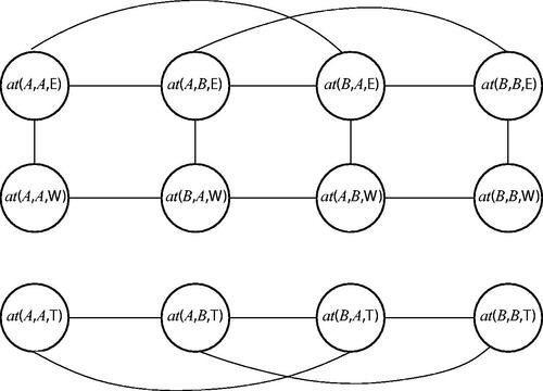
Figure 2. Example direction relations between relatum O₁ and locata O₂, F₁ and F₂.

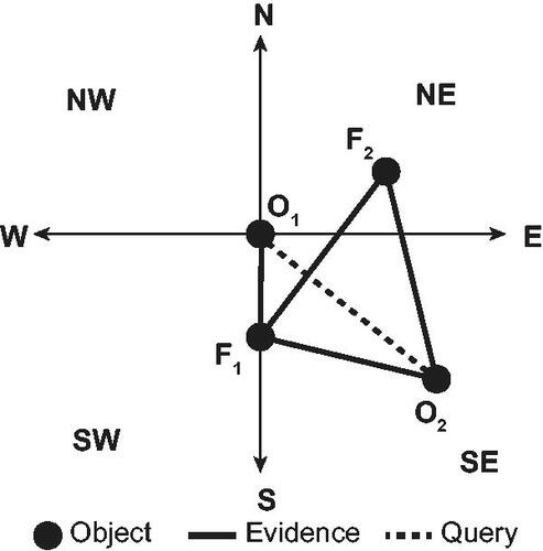
Figure 3. Results of experiment E1 with soft evidence SE1 $\mathit{dir}(O_2,O_1,\mathsf{SE})$ with scenarios S1–3 with probabilities 1, 0.9 and 0.3, respectively.

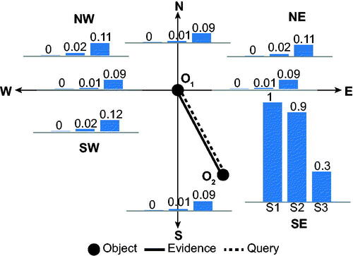
Figure 4. Results of experiment E2 with soft evidence SE2 $\mathit{dir}(F_1,O_1,\mathsf{S})$ and SE3 $\mathit{dir}(O_2,F_1,\mathsf{SE})$ $\mathit{dir}(O_2,O_1,\mathsf{SE})$ across scenarios S1–3 (Table 6).

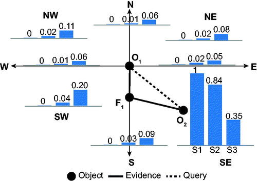
Figure 5. Results of experiment E3 with soft evidence SE2, SE4 and SE5 across scenarios S1–3 (Table 6).

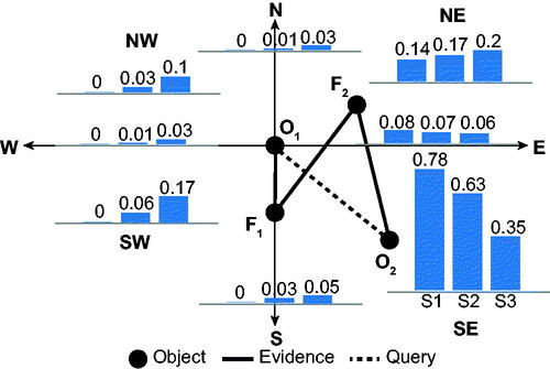
Figure 6. Examples of possible configuration of objects O₁, O₂, F₁ and F₂ consistent with evidence SE2, SE4 and SE5 in experiment E3 (Table 6).

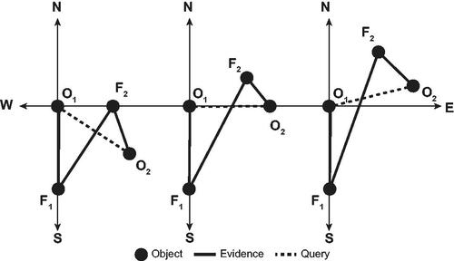
Figure 7. Results of experiment E4 with evidence SE2–5 across scenarios S1–3 (Table 6).

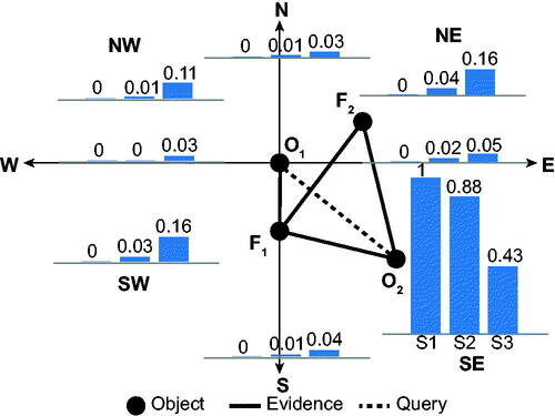
Figure 8. Examples of possible configuration of points O₁, O₂, F₁ and F₂ consistent with evidence SE3–6 in experiment E4 (Table 6).

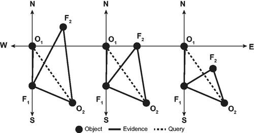
Figure 9. Results of experiment E5, extending experiment E2 with additional soft evidence for the direction relation between O₁ and F₁ (Table 7).

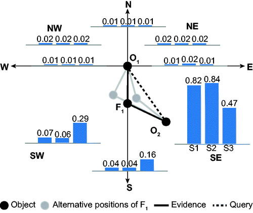
Figure 10. Three possible scenarios for inconsistent evidence where exactly one piece is neglected for each scenario (faded in graph).

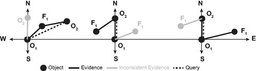
Figure 11. Results of experiment E6, extending experiment E2 with inconsistent evidence for the direction relation between O₁ and O₂, based on scenarios S1–3 in Table 8. The figure shows the spatial configuration from the left graph of Figure 10 only as an example (the configuration is strongly counter indicated by the resulting probabilities in scenario S3).

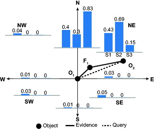
Table A1. MLN rule base for RCC-5.

Formula
$\mathit{rel}=\{DR,PO,PP,EQ,\mathit{PPI}\}$
$\mathit{rcc}(\mathit{region},\mathit{region},\mathit{rel}!)$
$\mathit{rcc}(a,b,DR)\Rightarrow \mathit{rcc}(b,a,DR).$
$\mathit{rcc}(a,b,PO)\Rightarrow \mathit{rcc}(b,a,PO).$
$\mathit{rcc}(a,b,PP)\Rightarrow \mathit{rcc}(b,a,\mathit{PPI}).$
$\mathit{rcc}(a,b,EQ)\Rightarrow \mathit{rcc}(b,a,EQ).$
$\mathit{rcc}(a,b,\mathit{PPI})\Rightarrow \mathit{rcc}(b,a,PP).$
$\mathit{rcc}(a,b,\mathit{rel})\wedge \mathit{rcc}(b,c,EQ)\Rightarrow \mathit{rcc}(a,c,\mathit{rel}).$
$\mathit{rcc}(a,b,DR)\wedge \mathit{rcc}(b,c,\mathit{PPI})\Rightarrow \mathit{rcc}(a,c,DR).$
$\mathit{rcc}(a,b,PO)\wedge \mathit{rcc}(b,c,PP)\Rightarrow \mathit{rcc}(a,c,PO)\vee \mathit{rcc}(a,c,PP).$
$\mathit{rcc}(a,b,PP)\wedge \mathit{rcc}(b,c,PP)\Rightarrow \mathit{rcc}(a,c,PP).$

Table A2. Exhaustive MLN rule base for CDC.

Formula
$\mathit{dir}(a,b,I)\Rightarrow b=a.$
$b=a\Rightarrow \mathit{dir}(a,b,I).$
$\mathit{dir}(a,b,N)\Rightarrow \mathit{dir}(b,a,S).$
$\mathit{dir}(b,a,S)\Rightarrow \mathit{dir}(a,b,N).$
$\mathit{dir}(a,b,W)\Rightarrow \mathit{dir}(b,a,E).$
$\mathit{dir}(b,a,E)\Rightarrow \mathit{dir}(a,b,W).$
$\mathit{dir}(a,b,NW)\Rightarrow \mathit{dir}(b,a,SE).$
$\mathit{dir}(b,a,SE)\Rightarrow \mathit{dir}(a,b,NW).$
$\mathit{dir}(a,b,NE)\Rightarrow \mathit{dir}(b,a,SW).$
$\mathit{dir}(b,a,SW)\Rightarrow \mathit{dir}(a,b,NE).$
$\mathit{dir}(a,b,r)\wedge \mathit{dir}(b,c,r)\Rightarrow \mathit{dir}(a,c,r).$
$\mathit{dir}(a,b,NW)\wedge \mathit{dir}(b,c,N)\Rightarrow \mathit{dir}(a,c,NW).$
$\mathit{dir}(a,b,NW)\wedge \mathit{dir}(b,c,W)\Rightarrow \mathit{dir}(a,c,NW).$
$\mathit{dir}(a,b,NW)\wedge \mathit{dir}(b,c,S)\Rightarrow \mathit{dir}(a,c,NW)\vee \mathit{dir}(a,c,W)\vee \mathit{dir}(a,c,SW).$
$\mathit{dir}(a,b,NW)\wedge \mathit{dir}(b,c,E)\Rightarrow \mathit{dir}(a,c,NW)\vee \mathit{dir}(a,c,N)\vee \mathit{dir}(a,c,NE).$
$\mathit{dir}(a,b,NW)\wedge \mathit{dir}(b,c,NE)\Rightarrow \mathit{dir}(a,c,N)\vee \mathit{dir}(a,c,NE)\vee \mathit{dir}(a,c,NW).$
$\mathit{dir}(a,b,NW)\wedge \mathit{dir}(b,c,SW)\Rightarrow \mathit{dir}(a,c,W)\vee \mathit{dir}(a,c,NW)\vee \mathit{dir}(a,c,SW).$
$\mathit{dir}(a,b,N)\wedge \mathit{dir}(b,c,E)\Rightarrow \mathit{dir}(a,c,NE).$
$\mathit{dir}(a,b,N)\wedge \mathit{dir}(b,c,W)\Rightarrow \mathit{dir}(a,c,NW).$
$\mathit{dir}(a,b,N)\wedge \mathit{dir}(b,c,S)\Rightarrow \mathit{dir}(a,c,S)\vee \mathit{dir}(a,c,N)\vee \mathit{dir}(a,c,I).$
$\mathit{dir}(a,b,N)\wedge \mathit{dir}(b,c,SE)\Rightarrow \mathit{dir}(a,c,E)\vee \mathit{dir}(a,c,SE)\vee \mathit{dir}(a,c,NE).$
$\mathit{dir}(a,b,N)\wedge \mathit{dir}(b,c,SW)\Rightarrow \mathit{dir}(a,c,W)\vee \mathit{dir}(a,c,NW)\vee \mathit{dir}(a,c,SW).$
$\mathit{dir}(a,b,N)\wedge \mathit{dir}(b,c,NE)\Rightarrow \mathit{dir}(a,c,NE).$
$\mathit{dir}(a,b,N)\wedge \mathit{dir}(b,c,NW)\Rightarrow \mathit{dir}(a,c,NW).$
$\mathit{dir}(a,b,NE)\wedge \mathit{dir}(b,c,N)\Rightarrow \mathit{dir}(a,c,NE).$
$\mathit{dir}(a,b,NE)\wedge \mathit{dir}(b,c,W)\Rightarrow \mathit{dir}(a,c,NW)\vee \mathit{dir}(a,c,N)\vee \mathit{dir}(a,c,NE).$
$\mathit{dir}(a,b,NE)\wedge \mathit{dir}(b,c,S)\Rightarrow \mathit{dir}(a,c,NE)\vee \mathit{dir}(a,c,E)\vee \mathit{dir}(a,c,SE).$
$\mathit{dir}(a,b,NE)\wedge \mathit{dir}(b,c,E)\Rightarrow \mathit{dir}(a,c,NE).$
$\mathit{dir}(a,b,NE)\wedge \mathit{dir}(b,c,NW)\Rightarrow \mathit{dir}(a,c,NW)\vee \mathit{dir}(a,c,N)\vee \mathit{dir}(a,c,NE).$
$\mathit{dir}(a,b,NE)\wedge \mathit{dir}(b,c,SE)\Rightarrow \mathit{dir}(a,c,NE)\vee \mathit{dir}(a,c,E)\vee \mathit{dir}(a,c,SE).$
$\mathit{dir}(a,b,E)\wedge \mathit{dir}(b,c,N)\Rightarrow \mathit{dir}(a,c,NE).$
$\mathit{dir}(a,b,E)\wedge \mathit{dir}(b,c,S)\Rightarrow \mathit{dir}(a,c,SE).$
$\mathit{dir}(a,b,E)\wedge \mathit{dir}(b,c,W)\Rightarrow \mathit{dir}(a,c,E)\vee \mathit{dir}(a,c,W)\vee \mathit{dir}(a,c,I).$
$\mathit{dir}(a,b,E)\wedge \mathit{dir}(b,c,NW)\Rightarrow \mathit{dir}(a,c,N)\vee \mathit{dir}(a,c,NE)\vee \mathit{dir}(a,c,NW).$
$\mathit{dir}(a,b,E)\wedge \mathit{dir}(b,c,NE)\Rightarrow \mathit{dir}(a,c,NE).$
$\mathit{dir}(a,b,E)\wedge \mathit{dir}(b,c,SW)\Rightarrow \mathit{dir}(a,c,S)\vee \mathit{dir}(a,c,SE)\vee \mathit{dir}(a,c,SW).$
$\mathit{dir}(a,b,E)\wedge \mathit{dir}(b,c,SE)\Rightarrow \mathit{dir}(a,c,SE).$
$\mathit{dir}(a,b,SE)\wedge \mathit{dir}(b,c,N)\Rightarrow \mathit{dir}(a,c,NE)\vee \mathit{dir}(a,c,E)\vee \mathit{dir}(a,c,SE).$
$\mathit{dir}(a,b,SE)\wedge \mathit{dir}(b,c,W)\Rightarrow \mathit{dir}(a,c,SW)\vee \mathit{dir}(a,c,S)\vee \mathit{dir}(a,c,SE).$
$\mathit{dir}(a,b,SE)\wedge \mathit{dir}(b,c,S)\Rightarrow \mathit{dir}(a,c,SE).$
$\mathit{dir}(a,b,SE)\wedge \mathit{dir}(b,c,E)\Rightarrow \mathit{dir}(a,c,SE).$
$\mathit{dir}(a,b,SE)\wedge \mathit{dir}(b,c,NE)\Rightarrow \mathit{dir}(a,c,NE)\vee \mathit{dir}(a,c,E)\vee \mathit{dir}(a,c,SE).$
$\mathit{dir}(a,b,SE)\wedge \mathit{dir}(b,c,SW)\Rightarrow \mathit{dir}(a,c,SE)\vee \mathit{dir}(a,c,S)\vee \mathit{dir}(a,c,SW).$
$\mathit{dir}(a,b,S)\wedge \mathit{dir}(b,c,E)\Rightarrow \mathit{dir}(a,c,SE).$
$\mathit{dir}(a,b,S)\wedge \mathit{dir}(b,c,W)\Rightarrow \mathit{dir}(a,c,SW).$
$\mathit{dir}(a,b,S)\wedge \mathit{dir}(b,c,N)\Rightarrow \mathit{dir}(a,c,S)\vee \mathit{dir}(a,c,N)\vee \mathit{dir}(a,c,I).$
$\mathit{dir}(a,b,S)\wedge \mathit{dir}(b,c,NE)\Rightarrow \mathit{dir}(a,c,E)\vee \mathit{dir}(a,c,SE)\vee \mathit{dir}(a,c,NE).$
$\mathit{dir}(a,b,S)\wedge \mathit{dir}(b,c,NW)\Rightarrow \mathit{dir}(a,c,W)\vee \mathit{dir}(a,c,NW)\vee \mathit{dir}(a,c,SW).$
$\mathit{dir}(a,b,S)\wedge \mathit{dir}(b,c,SE)\Rightarrow \mathit{dir}(a,c,SE).$
$\mathit{dir}(a,b,S)\wedge \mathit{dir}(b,c,SW)\Rightarrow \mathit{dir}(a,c,SW).$
$\mathit{dir}(a,b,SW)\wedge \mathit{dir}(b,c,S)\Rightarrow \mathit{dir}(a,c,SW).$
$\mathit{dir}(a,b,SW)\wedge \mathit{dir}(b,c,W)\Rightarrow \mathit{dir}(a,c,SW).$
$\mathit{dir}(a,b,SW)\wedge \mathit{dir}(b,c,N)\Rightarrow \mathit{dir}(a,c,NE)\vee \mathit{dir}(a,c,E)\vee \mathit{dir}(a,c,SE).$
$\mathit{dir}(a,b,SW)\wedge \mathit{dir}(b,c,E)\Rightarrow \mathit{dir}(a,c,SW)\vee \mathit{dir}(a,c,S)\vee \mathit{dir}(a,c,SE).$
$\mathit{dir}(a,b,SW)\wedge \mathit{dir}(b,c,NW)\Rightarrow \mathit{dir}(a,c,NW)\vee \mathit{dir}(a,c,W)\vee \mathit{dir}(a,c,SW).$
$\mathit{dir}(a,b,SW)\wedge \mathit{dir}(b,c,SE)\Rightarrow \mathit{dir}(a,c,SE)\vee \mathit{dir}(a,c,S)\vee \mathit{dir}(a,c,SW).$
$\mathit{dir}(a,b,E)\wedge \mathit{dir}(b,c,N)\Rightarrow \mathit{dir}(a,c,NE).$
$\mathit{dir}(a,b,E)\wedge \mathit{dir}(b,c,S)\Rightarrow \mathit{dir}(a,c,SE).$
$\mathit{dir}(a,b,E)\wedge \mathit{dir}(b,c,W)\Rightarrow \mathit{dir}(a,c,E)\vee \mathit{dir}(a,c,W)\vee \mathit{dir}(a,c,I).$
$\mathit{dir}(a,b,E)\wedge \mathit{dir}(b,c,NW)\Rightarrow \mathit{dir}(a,c,N)\vee \mathit{dir}(a,c,NE)\vee \mathit{dir}(a,c,NW).$
$\mathit{dir}(a,b,E)\wedge \mathit{dir}(b,c,NE)\Rightarrow \mathit{dir}(a,c,NE).$
$\mathit{dir}(a,b,E)\wedge \mathit{dir}(b,c,SW)\Rightarrow \mathit{dir}(a,c,S)\vee \mathit{dir}(a,c,SE)\vee \mathit{dir}(a,c,SW).$
$\mathit{dir}(a,b,E)\wedge \mathit{dir}(b,c,SE)\Rightarrow \mathit{dir}(a,c,SE).$
$\mathit{dir}(a,b,W)\wedge \mathit{dir}(b,c,N)\Rightarrow \mathit{dir}(a,c,NW).$
$\mathit{dir}(a,b,W)\wedge \mathit{dir}(b,c,S)\Rightarrow \mathit{dir}(a,c,SW).$
$\mathit{dir}(a,b,W)\wedge \mathit{dir}(b,c,E)\Rightarrow \mathit{dir}(a,c,W)\vee \mathit{dir}(a,c,E)\vee \mathit{dir}(a,c,I).$
$\mathit{dir}(a,b,W)\wedge \mathit{dir}(b,c,NE)\Rightarrow \mathit{dir}(a,c,N)\vee \mathit{dir}(a,c,NW)\vee \mathit{dir}(a,c,NE).$
$\mathit{dir}(a,b,W)\wedge \mathit{dir}(b,c,SE)\Rightarrow \mathit{dir}(a,c,S)\vee \mathit{dir}(a,c,SW)\vee \mathit{dir}(a,c,SE).$
$\mathit{dir}(a,b,W)\wedge \mathit{dir}(b,c,NW)\Rightarrow \mathit{dir}(a,c,NW).$
$\mathit{dir}(a,b,W)\wedge \mathit{dir}(b,c,SW)\Rightarrow \mathit{dir}(a,c,SW).$

Table A3. MLN rule base for Allen’s interval algebra.

Formula
$\mathit{rel}=\{\mathit{Before},\mathit{After},\mathit{Equal},\mathit{Meets},\mathit{MeetsInverse},\mathit{Overlaps},\mathit{OverlapsInverse},\mathit{During},\mathit{DuringInverse},\mathit{Starts},\mathit{StartsInverse},\mathit{Finishes},\mathit{FinishesInverse}\}$
$lr=\{L,R,I\}$
$at(\mathit{timepoint},\mathit{timepoint},lr!)$
$\mathit{aia}(\mathit{segment},\mathit{segment},\mathit{rel}!)$
$\mathit{hasStart}(\mathit{segment},\mathit{timepoint}!)$
$\mathit{hasEnd}(\mathit{segment},\mathit{timepoint}!)$
$at(a,a,I).$
$at(a,b,I)\Rightarrow at(b,a,I).$
$at(a,b,L)\Rightarrow at(b,a,R).$
$at(a,b,R)\Rightarrow at(b,a,L).$
$at(a,b,r)\wedge at(b,c,I)\Rightarrow at(a,c,r).$
$at(a,b,r)\wedge at(b,c,r)\Rightarrow at(a,c,r).$
$at(a,b,L)\wedge at(b,c,R)\Rightarrow at(a,c,R)\vee at(a,c,L)\vee at(a,c,I).$
$\mathit{hasStart}(\mathit{seg}1,s1)\wedge \mathit{hasEnd}(\mathit{seg}1,e1)\Rightarrow at(s1,e1,L).$
$\mathit{hasStart}(\mathit{seg}1,s1)\wedge \mathit{hasEnd}(\mathit{seg}1,e1)\wedge \mathit{hasStart}(\mathit{seg}2,s2)\wedge \mathit{hasEnd}(\mathit{seg}2,e2)\wedge at(e1,s2,L)\Rightarrow \mathit{aia}(\mathit{seg}1,\mathit{seg}2,\mathit{Before}).$
$\mathit{hasStart}(\mathit{seg}1,s1)\wedge \mathit{hasEnd}(\mathit{seg}1,e1)\wedge \mathit{hasStart}(\mathit{seg}2,s2)\wedge \mathit{hasEnd}(\mathit{seg}2,e2)\wedge \mathit{aia}(\mathit{seg}1,\mathit{seg}2,\mathit{Before})\Rightarrow at(e1,s2,L).$
$\mathit{hasStart}(\mathit{seg}1,s1)\wedge \mathit{hasEnd}(\mathit{seg}1,e1)\wedge \mathit{hasStart}(\mathit{seg}2,s2)\wedge \mathit{hasEnd}(\mathit{seg}2,e2)\wedge at(e2,s1,L)\Rightarrow \mathit{aia}(\mathit{seg}1,\mathit{seg}2,\mathit{After}).$
$\mathit{hasStart}(\mathit{seg}1,s1)\wedge \mathit{hasEnd}(\mathit{seg}1,e1)\wedge \mathit{hasStart}(\mathit{seg}2,s2)\wedge \mathit{hasEnd}(\mathit{seg}2,e2)\wedge \mathit{aia}(\mathit{seg}1,\mathit{seg}2,\mathit{After})\Rightarrow at(e2,s1,L).$
$\mathit{hasStart}(\mathit{seg}1,s1)\wedge \mathit{hasEnd}(\mathit{seg}1,e1)\wedge \mathit{hasStart}(\mathit{seg}2,s2)\wedge \mathit{hasEnd}(\mathit{seg}2,e2)\wedge at(s1,s2,I)\wedge at(e1,e2,I)\Rightarrow \mathit{aia}(\mathit{seg}1,\mathit{seg}2,\mathit{Equal}).$
$\mathit{hasStart}(\mathit{seg}1,s1)\wedge \mathit{hasEnd}(\mathit{seg}1,e1)\wedge \mathit{hasStart}(\mathit{seg}2,s2)\wedge \mathit{hasEnd}(\mathit{seg}2,e2)\wedge \mathit{aia}(\mathit{seg}1,\mathit{seg}2,\mathit{Equal})\Rightarrow at(s1,s2,I).$
$\mathit{hasStart}(\mathit{seg}1,s1)\wedge \mathit{hasEnd}(\mathit{seg}1,e1)\wedge \mathit{hasStart}(\mathit{seg}2,s2)\wedge \mathit{hasEnd}(\mathit{seg}2,e2)\wedge \mathit{aia}(\mathit{seg}1,\mathit{seg}2,\mathit{Equal})\Rightarrow at(e1,e2,I).$
$\mathit{hasStart}(\mathit{seg}1,s1)\wedge \mathit{hasEnd}(\mathit{seg}1,e1)\wedge \mathit{hasStart}(\mathit{seg}2,s2)\wedge \mathit{hasEnd}(\mathit{seg}2,e2)\wedge at(e1,s2,I)\Rightarrow \mathit{aia}(\mathit{seg}1,\mathit{seg}2,\mathit{Meets}).$
$\mathit{hasStart}(\mathit{seg}1,s1)\wedge \mathit{hasEnd}(\mathit{seg}1,e1)\wedge \mathit{hasStart}(\mathit{seg}2,s2)\wedge \mathit{hasEnd}(\mathit{seg}2,e2)\wedge \mathit{aia}(\mathit{seg}1,\mathit{seg}2,\mathit{Meets})\Rightarrow at(e1,s2,I).$
$\mathit{hasStart}(\mathit{seg}1,s1)\wedge \mathit{hasEnd}(\mathit{seg}1,e1)\wedge \mathit{hasStart}(\mathit{seg}2,s2)\wedge \mathit{hasEnd}(\mathit{seg}2,e2)\wedge at(e2,s1,I)\Rightarrow \mathit{aia}(\mathit{seg}1,\mathit{seg}2,\mathit{MeetsInverse}).$
$\mathit{hasStart}(\mathit{seg}1,s1)\wedge \mathit{hasEnd}(\mathit{seg}1,e1)\wedge \mathit{hasStart}(\mathit{seg}2,s2)\wedge \mathit{hasEnd}(\mathit{seg}2,e2)\wedge \mathit{aia}(\mathit{seg}1,\mathit{seg}2,\mathit{MeetsInverse})\Rightarrow at(e2,s1,I).$
$\mathit{hasStart}(\mathit{seg}1,s1)\wedge \mathit{hasEnd}(\mathit{seg}1,e1)\wedge \mathit{hasStart}(\mathit{seg}2,s2)\wedge \mathit{hasEnd}(\mathit{seg}2,e2)\wedge at(s1,e2,L)\wedge at(s2,e1,L)\wedge at(s1,s2,L)\Rightarrow \mathit{aia}(\mathit{seg}1,\mathit{seg}2,\mathit{Overlaps}).$
$\mathit{hasStart}(\mathit{seg}1,s1)\wedge \mathit{hasEnd}(\mathit{seg}1,e1)\wedge \mathit{hasStart}(\mathit{seg}2,s2)\wedge \mathit{hasEnd}(\mathit{seg}2,e2)\wedge \mathit{aia}(\mathit{seg}1,\mathit{seg}2,\mathit{Overlaps})\Rightarrow at(s1,e2,L).$
$\mathit{hasStart}(\mathit{seg}1,s1)\wedge \mathit{hasEnd}(\mathit{seg}1,e1)\wedge \mathit{hasStart}(\mathit{seg}2,s2)\wedge \mathit{hasEnd}(\mathit{seg}2,e2)\wedge \mathit{aia}(\mathit{seg}1,\mathit{seg}2,\mathit{Overlaps})\Rightarrow at(s2,e1,L).$
$\mathit{hasStart}(\mathit{seg}1,s1)\wedge \mathit{hasEnd}(\mathit{seg}1,e1)\wedge \mathit{hasStart}(\mathit{seg}2,s2)\wedge \mathit{hasEnd}(\mathit{seg}2,e2)\wedge \mathit{aia}(\mathit{seg}1,\mathit{seg}2,\mathit{Overlaps})\Rightarrow at(s1,s2,L).$
$\mathit{hasStart}(\mathit{seg}1,s1)\wedge \mathit{hasEnd}(\mathit{seg}1,e1)\wedge \mathit{hasStart}(\mathit{seg}2,s2)\wedge \mathit{hasEnd}(\mathit{seg}2,e2)\wedge at(s1,e2,L)\wedge at(s2,e1,L)\wedge at(s1,s2,R)\Rightarrow \mathit{aia}(\mathit{seg}1,\mathit{seg}2,\mathit{OverlapsInverse}).$
$\mathit{hasStart}(\mathit{seg}1,s1)\wedge \mathit{hasEnd}(\mathit{seg}1,e1)\wedge \mathit{hasStart}(\mathit{seg}2,s2)\wedge \mathit{hasEnd}(\mathit{seg}2,e2)\wedge \mathit{aia}(\mathit{seg}1,\mathit{seg}2,\mathit{OverlapsInverse})\Rightarrow at(s1,e2,L).$
$\mathit{hasStart}(\mathit{seg}1,s1)\wedge \mathit{hasEnd}(\mathit{seg}1,e1)\wedge \mathit{hasStart}(\mathit{seg}2,s2)\wedge \mathit{hasEnd}(\mathit{seg}2,e2)\wedge \mathit{aia}(\mathit{seg}1,\mathit{seg}2,\mathit{OverlapsInverse})\Rightarrow at(s2,e1,L).$
$\mathit{hasStart}(\mathit{seg}1,s1)\wedge \mathit{hasEnd}(\mathit{seg}1,e1)\wedge \mathit{hasStart}(\mathit{seg}2,s2)\wedge \mathit{hasEnd}(\mathit{seg}2,e2)\wedge \mathit{aia}(\mathit{seg}1,\mathit{seg}2,\mathit{OverlapsInverse})\Rightarrow at(s1,s2,R).$
$\mathit{hasStart}(\mathit{seg}1,s1)\wedge \mathit{hasEnd}(\mathit{seg}1,e1)\wedge \mathit{hasStart}(\mathit{seg}2,s2)\wedge \mathit{hasEnd}(\mathit{seg}2,e2)\wedge at(s1,s2,R)\wedge at(e1,e2,L)\Rightarrow \mathit{aia}(\mathit{seg}1,\mathit{seg}2,\mathit{During}).$
$\mathit{hasStart}(\mathit{seg}1,s1)\wedge \mathit{hasEnd}(\mathit{seg}1,e1)\wedge \mathit{hasStart}(\mathit{seg}2,s2)\wedge \mathit{hasEnd}(\mathit{seg}2,e2)\wedge \mathit{aia}(\mathit{seg}1,\mathit{seg}2,\mathit{During})\Rightarrow at(s1,s2,R).$
$\mathit{hasStart}(\mathit{seg}1,s1)\wedge \mathit{hasEnd}(\mathit{seg}1,e1)\wedge \mathit{hasStart}(\mathit{seg}2,s2)\wedge \mathit{hasEnd}(\mathit{seg}2,e2)\wedge \mathit{aia}(\mathit{seg}1,\mathit{seg}2,\mathit{During})\Rightarrow at(e1,e2,L).$
$\mathit{hasStart}(\mathit{seg}1,s1)\wedge \mathit{hasEnd}(\mathit{seg}1,e1)\wedge \mathit{hasStart}(\mathit{seg}2,s2)\wedge \mathit{hasEnd}(\mathit{seg}2,e2)\wedge at(s1,s2,L)\wedge at(e1,e2,R)\Rightarrow \mathit{aia}(\mathit{seg}1,\mathit{seg}2,\mathit{DuringInverse}).$
$\mathit{hasStart}(\mathit{seg}1,s1)\wedge \mathit{hasEnd}(\mathit{seg}1,e1)\wedge \mathit{hasStart}(\mathit{seg}2,s2)\wedge \mathit{hasEnd}(\mathit{seg}2,e2)\wedge \mathit{aia}(\mathit{seg}1,\mathit{seg}2,\mathit{DuringInverse})\Rightarrow at(e1,e2,R).$
$\mathit{hasStart}(\mathit{seg}1,s1)\wedge \mathit{hasEnd}(\mathit{seg}1,e1)\wedge \mathit{hasStart}(\mathit{seg}2,s2)\wedge \mathit{hasEnd}(\mathit{seg}2,e2)\wedge \mathit{aia}(\mathit{seg}1,\mathit{seg}2,\mathit{DuringInverse})\Rightarrow at(s1,s2,L).$
$\mathit{hasStart}(\mathit{seg}1,s1)\wedge \mathit{hasEnd}(\mathit{seg}1,e1)\wedge \mathit{hasStart}(\mathit{seg}2,s2)\wedge \mathit{hasEnd}(\mathit{seg}2,e2)\wedge at(s1,s2,I)\wedge at(e1,e2,L)\Rightarrow \mathit{aia}(\mathit{seg}1,\mathit{seg}2,\mathit{Starts}).$
$\mathit{hasStart}(\mathit{seg}1,s1)\wedge \mathit{hasEnd}(\mathit{seg}1,e1)\wedge \mathit{hasStart}(\mathit{seg}2,s2)\wedge \mathit{hasEnd}(\mathit{seg}2,e2)\wedge \mathit{aia}(\mathit{seg}1,\mathit{seg}2,\mathit{Starts})\Rightarrow at(s1,s2,I).$
$\mathit{hasStart}(\mathit{seg}1,s1)\wedge \mathit{hasEnd}(\mathit{seg}1,e1)\wedge \mathit{hasStart}(\mathit{seg}2,s2)\wedge \mathit{hasEnd}(\mathit{seg}2,e2)\wedge \mathit{aia}(\mathit{seg}1,\mathit{seg}2,\mathit{Starts})\Rightarrow at(e1,e2,L).$
$\mathit{hasStart}(\mathit{seg}1,s1)\wedge \mathit{hasEnd}(\mathit{seg}1,e1)\wedge \mathit{hasStart}(\mathit{seg}2,s2)\wedge \mathit{hasEnd}(\mathit{seg}2,e2)\wedge at(s1,s2,I)\wedge at(e1,e2,R)\Rightarrow \mathit{aia}(\mathit{seg}1,\mathit{seg}2,\mathit{StartsInverse}).$
$\mathit{hasStart}(\mathit{seg}1,s1)\wedge \mathit{hasEnd}(\mathit{seg}1,e1)\wedge \mathit{hasStart}(\mathit{seg}2,s2)\wedge \mathit{hasEnd}(\mathit{seg}2,e2)\wedge \mathit{aia}(\mathit{seg}1,\mathit{seg}2,\mathit{StartsInverse})\Rightarrow at(s1,s2,I).$
$\mathit{hasStart}(\mathit{seg}1,s1)\wedge \mathit{hasEnd}(\mathit{seg}1,e1)\wedge \mathit{hasStart}(\mathit{seg}2,s2)\wedge \mathit{hasEnd}(\mathit{seg}2,e2)\wedge \mathit{aia}(\mathit{seg}1,\mathit{seg}2,\mathit{StartsInverse})\Rightarrow at(e1,e2,R).$
$\mathit{hasStart}(\mathit{seg}1,s1)\wedge \mathit{hasEnd}(\mathit{seg}1,e1)\wedge \mathit{hasStart}(\mathit{seg}2,s2)\wedge \mathit{hasEnd}(\mathit{seg}2,e2)\wedge at(s1,s2,R)\wedge at(e1,e2,I)\Rightarrow \mathit{aia}(\mathit{seg}1,\mathit{seg}2,\mathit{Finishes}).$
$\mathit{hasStart}(\mathit{seg}1,s1)\wedge \mathit{hasEnd}(\mathit{seg}1,e1)\wedge \mathit{hasStart}(\mathit{seg}2,s2)\wedge \mathit{hasEnd}(\mathit{seg}2,e2)\wedge \mathit{aia}(\mathit{seg}1,\mathit{seg}2,\mathit{Finishes})\Rightarrow at(s1,s2,R).$
$\mathit{hasStart}(\mathit{seg}1,s1)\wedge \mathit{hasEnd}(\mathit{seg}1,e1)\wedge \mathit{hasStart}(\mathit{seg}2,s2)\wedge \mathit{hasEnd}(\mathit{seg}2,e2)\wedge \mathit{aia}(\mathit{seg}1,\mathit{seg}2,\mathit{Finishes})\Rightarrow at(e1,e2,I).$
$\mathit{hasStart}(\mathit{seg}1,s1)\wedge \mathit{hasEnd}(\mathit{seg}1,e1)\wedge \mathit{hasStart}(\mathit{seg}2,s2)\wedge \mathit{hasEnd}(\mathit{seg}2,e2)\wedge at(s1,s2,L)\wedge at(e1,e2,I)\Rightarrow \mathit{aia}(\mathit{seg}1,\mathit{seg}2,\mathit{FinishesInverse}).$
$\mathit{hasStart}(\mathit{seg}1,s1)\wedge \mathit{hasEnd}(\mathit{seg}1,e1)\wedge \mathit{hasStart}(\mathit{seg}2,s2)\wedge \mathit{hasEnd}(\mathit{seg}2,e2)\wedge \mathit{aia}(\mathit{seg}1,\mathit{seg}2,\mathit{FinishesInverse})\Rightarrow at(s1,s2,L).$
$\mathit{hasStart}(\mathit{seg}1,s1)\wedge \mathit{hasEnd}(\mathit{seg}1,e1)\wedge \mathit{hasStart}(\mathit{seg}2,s2)\wedge \mathit{hasEnd}(\mathit{seg}2,e2)\wedge \mathit{aia}(\mathit{seg}1,\mathit{seg}2,\mathit{FinishesInverse})\Rightarrow at(e1,e2,I).$

Table 1. Illustration of RCC relations.

RCC-8	DC	EC	PO	TPP	NTPP	EQ	TPPi	NTPPi
RCC-5	DR		PO	PP		EQ	PPi

Table 2. MLN rule-base for east–west calculus.

ID	Formula
F1	$at(b,a,\mathsf{E})\iff at(a,b,\mathsf{W})$
F2	$at(b,a,\mathsf{T})\iff at(a,b,\mathsf{T})$
F3	$at(b,a,r)\wedge at(c,b,r)\Rightarrow at(c,a,r)$

Table 3. Truth values for predicates in possible worlds W_a, W_b and W_c.

Ground predicate	Wa	Wb	Wc
$at(A,A,\mathsf{E})$	0	0	0
$at(A,A,\mathsf{W})$	0	0	0
$at(A,A,\mathsf{T})$	1	1	1
$at(A,B,\mathsf{E})$	1	0	1
$at(A,B,\mathsf{W})$	0	1	0
$at(A,B,\mathsf{T})$	0	0	0
$at(B,A,\mathsf{E})$	0	1	1
$at(B,A,\mathsf{W})$	1	0	0
$at(B,A,\mathsf{T})$	0	0	0
$at(B,B,\mathsf{E})$	0	0	0
$at(B,B,\mathsf{W})$	0	0	0
$at(B,B,\mathsf{T})$	1	1	1

Table 4. Truth values for groundings of formula F₁ in the world W_a, W_b and W_c.

Grounding	Wa	Wb	Wc
$at(A,A,\mathsf{E})\iff at(A,A,\mathsf{W})$	1	1	1
$at(A,B,\mathsf{E})\iff at(B,A,\mathsf{W})$	1	1	0
$at(B,A,\mathsf{E})\iff at(A,B,\mathsf{W})$	1	1	0
$at(B,B,\mathsf{E})\iff at(B,B,\mathsf{W})$	1	1	1

Table 5. MLN rule base for point-based CDC relation.

ID	Formula
C1	$\mathit{dir}(b,a,\mathsf{I})\iff b=a$
C2	$\mathit{dir}(b,a,\mathsf{N})\iff \mathit{dir}(a,b,\mathsf{S})$
C3	$\mathit{dir}(b,a,\mathsf{W})\iff \mathit{dir}(a,b,\mathsf{E})$
C4	$\mathit{dir}(b,a,\mathsf{NW})\iff \mathit{dir}(a,b,\mathsf{SE})$
C5	$\mathit{dir}(b,a,\mathsf{NE})\iff \mathit{dir}(a,b,\mathsf{SW})$
C6	$\mathit{dir}(b,a,\mathsf{N})\wedge \mathit{dir}(c,b,\mathsf{N})\Rightarrow \mathit{dir}(c,a,\mathsf{N})$
C7	$\mathit{dir}(b,a,\mathsf{NW})\wedge \mathit{dir}(c,b,\mathsf{NW})\Rightarrow \mathit{dir}(c,a,\mathsf{NW})$
C8	$\mathit{dir}(b,a,\mathsf{NE})\wedge \mathit{dir}(c,b,\mathsf{NE})\Rightarrow \mathit{dir}(c,a,\mathsf{NE})$
C9	$\mathit{dir}(b,a,\mathsf{NW})\wedge \mathit{dir}(c,b,\mathsf{N})\Rightarrow \mathit{dir}(c,a,\mathsf{NW})$
C10	$\mathit{dir}(b,a,\mathsf{NW})\wedge \mathit{dir}(c,b,\mathsf{W})\Rightarrow \mathit{dir}(c,a,\mathsf{NW})$
C11	$\mathit{dir}(b,a,\mathsf{SW})\wedge \mathit{dir}(c,b,\mathsf{S})\Rightarrow \mathit{dir}(c,a,\mathsf{SW})$
C12	$\mathit{dir}(b,a,\mathsf{SW})\wedge \mathit{dir}(c,b,\mathsf{W})\Rightarrow \mathit{dir}(c,a,\mathsf{SW})$
C13	$\mathit{dir}(b,a,\mathsf{N})\wedge \mathit{dir}(c,b,\mathsf{E})\Rightarrow \mathit{dir}(c,a,\mathsf{NE})$
C14	$\mathit{dir}(b,a,\mathsf{S})\wedge \mathit{dir}(c,b,\mathsf{E})\Rightarrow \mathit{dir}(c,a,\mathsf{SE})$
C15	$\mathit{dir}(b,a,\mathsf{N})\wedge \mathit{dir}(c,b,\mathsf{S})\Rightarrow \mathit{dir}(c,a,\mathsf{S})\vee \mathit{dir}(c,a,\mathsf{N})\vee \mathit{dir}(c,a,\mathsf{I})$
C16	$\mathit{dir}(b,a,\mathsf{W})\wedge \mathit{dir}(c,b,\mathsf{E})\Rightarrow \mathit{dir}(c,a,\mathsf{W})\vee \mathit{dir}(c,a,\mathsf{E})\vee \mathit{dir}(c,a,\mathsf{I})$
C17	$\mathit{dir}(b,a,\mathsf{NW})\wedge \mathit{dir}(c,b,\mathsf{NE})\Rightarrow \mathit{dir}(c,a,\mathsf{N})\vee \mathit{dir}(c,a,\mathsf{NE})\vee \mathit{dir}(c,a,\mathsf{NW})$
C18	$\mathit{dir}(b,a,\mathsf{NW})\wedge \mathit{dir}(c,b,\mathsf{SW})\Rightarrow \mathit{dir}(c,a,\mathsf{W})\vee \mathit{dir}(c,a,\mathsf{NW})\vee \mathit{dir}(c,a,\mathsf{SW})$
C19	$\mathit{dir}(b,a,\mathsf{N})\wedge \mathit{dir}(c,b,\mathsf{SE})\Rightarrow \mathit{dir}(c,a,\mathsf{E})\vee \mathit{dir}(c,a,\mathsf{SE})\vee \mathit{dir}(c,a,\mathsf{NE})$
C20	$\mathit{dir}(b,a,\mathsf{N})\wedge \mathit{dir}(c,b,\mathsf{SW})\Rightarrow \mathit{dir}(c,a,\mathsf{W})\vee \mathit{dir}(c,a,\mathsf{NW})\vee \mathit{dir}(c,a,\mathsf{SW})$
C21	$\mathit{dir}(b,a,\mathsf{S})\wedge \mathit{dir}(c,b,\mathsf{NE})\Rightarrow \mathit{dir}(c,a,\mathsf{E})\vee \mathit{dir}(c,a,\mathsf{SE})\vee \mathit{dir}(c,a,\mathsf{NE})$
C22	$\mathit{dir}(b,a,\mathsf{S})\wedge \mathit{dir}(c,b,\mathsf{NW})\Rightarrow \mathit{dir}(c,a,\mathsf{W})\vee \mathit{dir}(c,a,\mathsf{NW})\vee \mathit{dir}(c,a,\mathsf{SW})$
C23	$\mathit{dir}(b,a,\mathsf{E})\wedge \mathit{dir}(c,b,\mathsf{NW})\Rightarrow \mathit{dir}(c,a,\mathsf{N})\vee \mathit{dir}(c,a,\mathsf{NE})\vee \mathit{dir}(c,a,\mathsf{NW})$
C24	$\mathit{dir}(b,a,\mathsf{E})\wedge \mathit{dir}(c,b,\mathsf{SW})\Rightarrow \mathit{dir}(c,a,\mathsf{S})\vee \mathit{dir}(c,a,\mathsf{SE})\vee \mathit{dir}(c,a,\mathsf{SW})$
C25	$\mathit{dir}(b,a,\mathsf{W})\wedge \mathit{dir}(c,b,\mathsf{NE})\Rightarrow \mathit{dir}(c,a,\mathsf{N})\vee \mathit{dir}(c,a,\mathsf{NE})\vee \mathit{dir}(c,a,\mathsf{NW})$
C26	$\mathit{dir}(b,a,\mathsf{W})\wedge \mathit{dir}(c,b,\mathsf{SE})\Rightarrow \mathit{dir}(c,a,\mathsf{S})\vee \mathit{dir}(c,a,\mathsf{SE})\vee \mathit{dir}(c,a,\mathsf{SW})$

Table 6. Experimental setup for experiments E1–4 with evidential statements SE1–5 and associated probability scenarios S1–3.

Exp. #	Ev. #	Predicate	Probability
			S1	S2	S3
E1	SE1	$\mathit{dir}(O_2,O_1,\mathsf{SE})$	1	0.9	0.3
E2	SE2	$\mathit{dir}(F_1,O_1,\mathsf{S})$	1	0.9	0.9
	SE3	$\mathit{dir}(O_2,F_1,\mathsf{SE})$	1	0.9	0.3
E3	SE2	$\mathit{dir}(F_1,O_1,\mathsf{S})$	1	0.9	0.9
	SE4	$\mathit{dir}(F_2,F_1,\mathsf{NE})$	1	0.9	0.9
	SE5	$\mathit{dir}(O_2,F_2,\mathsf{SE})$	1	0.9	0.3
E4	SE2	$\mathit{dir}(F_1,O_1,\mathsf{S})$	1	0.9	0.9
	SE3	$\mathit{dir}(O_2,F_1,\mathsf{SE})$	1	0.9	0.3
	SE4	$\mathit{dir}(F_2,F_1,\mathsf{NE})$	1	0.9	0.9
	SE5	$\mathit{dir}(O_2,F_2,\mathsf{SE})$	1	0.9	0.3

Table 7. Experimental setup for experiment E5, extending experiment E2 with additional soft evidence SE2a and SE2b and associated probability scenarios S1–3.

Exp. #	Ev. #	Predicate	Probability
			S1	S2	S3
E5	SE3	$\mathit{dir}(O_2,F_1,\mathsf{SE})$	0.9	0.9	0.9
	SE2	$\mathit{dir}(F_1,O_1,\mathsf{S})$	0.8	0.2	0.2
	SE2a	$\mathit{dir}(F_1,O_1,\mathsf{SE})$	0.1	0.7	0.1
	SE2b	$\mathit{dir}(F_1,O_1,\mathsf{SW})$	0.1	0.1	0.7

Table 8. Experimental setup for experiment E6 with soft evidence SE6–8 and associated probability scenarios S1–3.

Exp. #	Ev. #	Predicate	Probability
			S1	S2	S3
E6	SE6	$\mathit{dir}(F_1,O_2,\mathsf{SW})$	0.4	0.9	0.4
	SE7	$\mathit{dir}(O_1,F_1,\mathsf{SW})$	0.9	0.9	0.9
	SE8	$\mathit{dir}(O_1,O_2,\mathsf{S})$	0.4	0.4	0.9

References

- Alevizos, E. and Artikis, A., 2018. A prototype for maritime event forecasting. In: Maritime Big Data workshop, Spezia, Italy, 19–24.
- Allen, J.F., 1983. Maintaining knowledge about temporal intervals. Communications of the ACM, 26 (11), 832–843.
- Balbiani, P., Condotta, J.-F., and Fariñas del Cerro, L., 1999. A new tractable subclass of the rectangle algebra. In: Proceedings of the 16th international joint conference on artificial intelligence (IJCAI), 442–447.
- Banerjee, P., Ranu, S., and Raghavan, S., 2014. Inferring uncertain trajectories from partial observations. In: Proceedings of the IEEE international conference on data mining. IEEE, 30–39.
- Bennett, B., 1994. Spatial reasoning with propositional logics. In: Principles of knowledge representation and reasoning. New York: Elsevier, 51–62.
- Brouard, C., et al., 2013. Learning a Markov logic network for supervised gene regulatory network inference. BMC Bioinformatics, 14 (1), 273.
- Bruns, H.T. and Egenhofer, M., 1996. Similarity of spatial scenes. In: Proceedings of the 7th international symposium on spatial data handling (SDH), 31–42.
- Chrisman, N.R., 1991. The error component in spatial data. Geographical Information Systems, 1 (12), 165–174.
- Cohn, A. and Gotts, M., 1996a. The ‘egg-yolk’ representation of regions with indeterminate boundaries. In: P.A. Burrough and A. Frank, eds. Geographic objects with indeterminate boundaries, vol. 2. Boca Raton, FL: CRC Press, 171–188.
- Cohn, A. and Gotts, N., 1996b. Representing spatial vagueness: a mereological approach. In: Proceedings of the fifth international conference on principles of knowledge representation and reasoning (KR96). Morgan Kaufmann.
- Cohn, A. and Hazarika, S., 2001. Qualitative spatial representation and reasoning: an overview. Fundamenta Informaticae, 46, 2–32.
- Cohn, A.G. and Renz, J., 2008. Qualitative spatial representation and reasoning. Foundations of Artificial Intelligence, 3, 551–596.
- Cohn, A.G., et al., 1997. Qualitative spatial representation and reasoning with the region connection calculus. Geoinformatica, 1 (3), 275–316.
- Cohn, A.G., et al., 2014. Reasoning about topological and cardinal direction relations between 2-dimensional spatial objects. Journal of Artificial Intelligence Research, 51, 493–532.
- Domingos, P., et al., 2008. Markov logic. In: L. De Raedt, et al., eds. Probabilistic inductive logic programming: theory and applications. Berlin: Springer, 92–117.
- Domingos, P. and Lowd, D., 2009. Markov logic: an interface layer for artificial intelligence. In: Number 1 in synthesis lectures on artificial intelligence and machine learning. Berlin: Morgan & Claypool Publishers.
- Duckham, M., 2008. Qualitative monitoring of dynamic spatial fields in geosensor networks. In: S. Shekhar and H. Xiong, eds. Encyclopedia of GIS. Berlin: Springer, 376–379.
- Duckham, M. and Worboys, M., 2001. Computational structure in three-valued nearness relations. In: International conference on spatial information theory (COSIT). Springer, 76–91.
- Dylla, F., et al., 2006. SparQ: a toolbox for qualitative spatial representation and reasoning. In: Qualitative constraint calculi: application and integration, workshop at KI, 79–90.
- Dylla, F., et al., 2018. A survey of qualitative spatial and temporal calculi: algebraic and computational properties. ACM Computing Surveys, 50 (1), 1–39.
- Emrich, T., et al., 2012. Querying uncertain spatio-temporal data. In: Proceedings of the 28th IEEE international conference on data engineering. IEEE, 354–365.
- Fisher, P.F., 1999. Chapter 13: models of uncertainty in spatial data. In: P. Longley, et al., eds., Geographical information systems. 2nd ed. New York: John Wiley & Sons.
- Frank, A.U., 1992. Qualitative spatial reasoning about distances and directions in geographic space. Journal of Visual Languages & Computing, 3 (4), 343–371.
- Freksa, C., 1991. Qualitative spatial reasoning. In: D.M. Mark, A.U. Frank, eds. Cognitive and linguistic aspects of geographic space. Berlin: Springer, 361–372.
- Freksa, C., 1992. Temporal reasoning based on semi-intervals. Artificial Intelligence, 54 (1–2), 199–227.
- Freksa, C., 2005. Using orientation information for qualitative spatial reasoning. In: Theories and methods of spatio-temporal reasoning in geographic space: international conference GIS—from space to territory. Springer, 162–178.
- Freksa, C. and Zimmermann, K., 1992. On the utilization of spatial structures for cognitively plausible and efficient reasoning. In: Proceedings of the IEEE international conference on systems, man, and cybernetics. IEEE, 261–266.
- Galton, A., 2000. Qualitative spatial change. Oxford, UK: Oxford University Press.
- Gatsoulis, Y., et al., 2016. Qsrlib: a software library for online acquisition of qualitative spatial relations from video. In: Workshop on Qualitative Reasoning (QR16) at IJCAI-16.
- Girlea, C.L. and Amir, E., 2015. Probabilistic region connection calculus. In: Proceedings of the AAAI spring symposium series, 66–70.
- Goyal, R. and Egenhofer, M., 2001. Similarity of cardinal directions. In: C. Jensen, et al., eds., Proceedings of the international symposium on advances in spatial and temporal databases (SSTD). Springer, 36–58.
- Guptill, S.C. and Morrison, J.L., eds., 1995. Elements of spatial data quality. New York: Elsevier.
- Hammersley, J.M. and Clifford, P.E., 1971. Markov random fields on finite graphs and lattices. Available from: http://www.statslab.cam.ac.uk/grg/books/hammfest/hamm-cliff.pdf. Unpublished manuscript.
- Isli, A. and Cohn, A.G., 1998. An algebra for cyclic ordering of 2D orientations. In: AAAI/IAAI, 643–649.
- Jain, D. and Beetz, M., 2010. Soft evidential update via Markov chain Monte Carlo inference. In: R. Dillmann, et al., eds., Proceedings of the 33rd annual German conference on AI (KI), volume 6359 of lecture notes in computer science. Springer, 280–290.
- Kautz, H., Selman, B., and Jiang, Y., 1997. A general stochastic approach to solving problems with hard and soft constraints. In: D. Du, J. Gu, and P.M. Pardalos, eds., Satisfiability problem: theory and applications, volume 35 of DIMACS series in discrete mathematics and theoretical computer science. Rhode Island: AMS Books, 573–585.
- Keefe, R. and Smith, P., 1996. Vagueness: a reader. Cambridge, MA: MIT Press.
- Khot, T., et al., 2011. Learning Markov logic networks via functional gradient boosting. In: Proceedings of the 11th IEEE international conference on data mining. IEEE, 320–329.
- Li, S., Liu, W., and Wang, S., 2013. Qualitative constraint satisfaction problems: an extended framework with landmarks. Artificial Intelligence, 201, 32–58.
- Li, S. and Ying, M., 2003. Region connection calculus: its models and composition table. Artificial Intelligence, 145 (1–2), 121–146.
- Ligozat, G., 2013. Qualitative spatial and temporal reasoning. San Francisco, CA: John Wiley & Sons.
- Loerch, U. and Guesgen, H.W., 1997. Qualitative spatial reasoning under uncertainty in geographical information systems. In: Proceedings of the IEEE international conference on systems, man, and cybernetics. IEEE, 2169–2174.
- Lowd, D. and Domingos, P., 2007. Efficient weight learning for Markov logic networks. In: Proceedings of the conference on knowledge discovery in databases (PKDD). Springer, 200–211.
- Moratz, R., 2017. Qualitative spatial reasoning. In: S. Shekhar, et al., eds. Encyclopedia of GIS. Berlin: Springer, 1700–1707.
- Mossakowski, T. and Moratz, R., 2012. Qualitative reasoning about relative direction of oriented points. Artificial Intelligence, 180–181, 34–45.
- Mossakowski, T. and Moratz, R., 2015. Relations between spatial calculi about directions and orientations. Journal of Artificial Intelligence Research, 54, 277–308.
- Nguyen, V., 2019. On combining probabilistic and semantic similarity-based methods toward off-domain reasoning for situational awareness. In: Proceedings of the 22nd international conference on information fusion, Ottawa, ON, Canada.
- Nguyen, V. and Mellor, L., 2020. Fuzzy MLNs and QSTAGs for activity recognition and modelling with RUSH. In: Proceedings of the 23rd international conference on information fusion (FUSION). IEEE, 1–8.
- Niu, F., et al., 2011. Tuffy: scaling up statistical inference in Markov logic networks using an RDBMS. arXiv preprint, abs/1104.3216.
- Petry, F.E., Robinson, V.B., and Cobb, M.A., 2005. Fuzzy modeling with spatial information for geographic problems. Berlin: Springer.
- Poon, H. and Domingos, P., 2006. Sound and efficient inference with probabilistic and deterministic dependencies. In: Proceedings of the National Conference on Artificial Intelligence, 458–463.
- Ragni, M., et al., 2016. Uncertain relational reasoning in the parietal cortex. Brain and Cognition, 104, 72–81.
- Randell, D.A., Cui, Z., and Cohn, A.G., 1992. A spatial logic based on regions and connection. In: B. Nebel, C. Rich, and W. Swartout, eds., Proceedings of the international conference principles of knowledge representation and reasoning (KR). San Mateo, CA: Morgan Kaufmann, 165–176.
- Renz, J. and Ligozat, G., 2005. Weak composition for qualitative spatial and temporal reasoning. In: Proceedings of the 11th international conference on principles and practice of constraint programming (CP). Springer, 534–548.
- Renz, J. and Nebel, B., 2001. Efficient methods for qualitative spatial reasoning. Journal of Artificial Intelligence Research, 15, 289–318.
- Richardson, M. and Domingos, P., 2006. Markov logic networks. Machine Learning, 62 (1–2), 107–136.
- Richardson, S., Domingos, P., and Poon, M.S.H., 2007. The Alchemy system for statistical relational AI: user manual (washington.edu). http://alchemy.cs.washington.edu/user-manual/manual.html
- Sabek, I., 2019. Adopting Markov logic networks for big spatial data and applications. In: Proceedings of the 45th international conference on very large data bases (VLDB) PhD workshop, Los Angeles, CA, 1–4.
- Sabek, I., Musleh, M., and Mokbel, M.F., 2019. Flash in action: scalable spatial data analysis using Markov logic networks. Proceedings of the VLDB Endowment, 12 (12), 1834–1837.
- Sakhanenko, N.A. and Galas, D.J., 2010. Markov logic networks in the analysis of genetic data. Journal of Computational Biology, 17 (11), 1491–1508.
- Sarkhel, S., et al., 2014. Lifted MAP inference for Markov logic networks. In: Artificial intelligence and statistics. PMLR, 859–867.
- Schlieder, C., 1995. Reasoning about ordering. In: International conference on spatial information theory (COSIT), volume 988 of lecture notes in computer science, 341–349.
- Schockaert, S., De Cock, M., and Kerre, E.E., 2009. Spatial reasoning in a fuzzy region connection calculus. Artificial Intelligence, 173 (2), 258–298.
- Schultz, C., Bhatt, M., and Suchan, J., 2016. Probabilistic spatial reasoning in constraint logic programming. In: S. Schockaert and P. Senellart, eds., Proceedings of the 10th international conference on scalable uncertainty management (SUM). Springer, 289–302.
- Scivos, A. and Nebel, B., 2001. Double-crossing: decidability and computational complexity of a qualitative calculus for navigation. In: International conference on spatial information theory (COSIT). Springer, 431–446.
- Sioutis, M. and Wolter, D., 2021. Qualitative spatial and temporal reasoning: current status and future challenges. In: Proceedings of the international joint conference on artificial intelligence (IJCAI), 4594–4601.
- Skiadopoulos, S. and Koubarakis, M., 2004. Composing cardinal direction relations. Artificial Intelligence, 152 (2), 143–171.
- Snidaro, L., Visentini, I., and Bryan, K., 2015. Fusing uncertain knowledge and evidence for maritime situational awareness via Markov logic networks. Information Fusion, 21, 159–172.
- Sun, Z., et al., 2017. Scalable learning and inference in Markov logic networks. International Journal of Approximate Reasoning, 82, 39–55.
- Tarski, A., 1941. On the calculus of relations. Journal of Symbolic Logic, 6 (3), 73–89.
- Tenorth, M., Jain, D., and Beetz, M., 2010. Knowledge representation for cognitive robots. KI – Künstliche Intelligenz, 24 (3), 233–240.
- Van de Weghe, N., et al., 2005. Representing moving objects in computer-based expert systems: the overtake event example. Expert Systems with Applications, 29 (4), 977–983.
- Van de Weghe, N., et al., 2006. A qualitative trajectory calculus as a basis for representing moving objects in geographical information systems. Control and Cybernetics, 35, 97–119.
- Varzi, A.C., 2001. Vagueness in geography. Philosophy & Geography, 4 (1), 49–65.
- Wallgrün, J.O., et al., 2006. Qualitative spatial representation and reasoning in the SparQ-toolbox. In: International conference on spatial cognition. Springer, 39–58.
- Wick, M., McCallum, A., and Miklau, G., 2010. Scalable probabilistic databases with factor graphs and MCMC. arXiv preprint, arXiv:1005.1934.
- Wolter, D. and Wallgrün, J.O., 2013. Qualitative spatial reasoning for applications: new challenges and the SparQ toolbox. In: Geographic information systems: concepts, methodologies, tools, and applications. IGI Global, 1639–1664.
- Worboys, M.F., 2001. Nearness relations in environmental space. International Journal of Geographical Information Science, 15 (7), 633–651.
- Worboys, M.F. and Clementini, E., 2001. Integration of imperfect spatial information. Journal of Visual Languages & Computing, 12 (1), 61–80.
- Zhu, R., et al., 2022. Reasoning over higher-order qualitative spatial relations via spatially explicit neural networks. International Journal of Geographical Information Science, 36 (11), 2194–2225.