What drives the geography of jobs in the US? Unpacking relatedness

ABSTRACT

There is ample evidence of regions diversifying in new occupations that are related to pre-existing activities in the region. However, it is still poorly understood through which mechanisms related diversification operates. To unpack relatedness, we distinguish between three mechanisms: complementarity (interdependent tasks), similarity (sharing similar skills) and local synergy (based on pure co-location). We propose a measure for each of these relatedness dimensions and assess their impact on the evolution of the occupational structure of 389 US Metropolitan Statistical Areas (MSA) for the period 2005–2016. Our findings show that new jobs appearing in MSA’s are related to existing ones, while those more likely to disappear are more unrelated to a city’s jobs’ portfolio. We found that all three relatedness dimensions matter, but local synergy shows the largest impact on entry and exit of jobs in US cities, thus being the strongest force of diversification.

KEYWORDS:

• Evolutionary economic geography
• regional capabilities
• jobs
• relatedness
• US cities

JEL:

• J24
• O18
• R10

1. Introduction

The 2008 crisis has led to unprecedented job losses and the destruction of human capital in many regions worldwide. Notwithstanding, projections are that it can get much worse. Technological change, automation, and offshoring of jobs are leaving their marks in the local workforce, and we can expect in the near future a massive and generalised decrease in labour demand due to skill mismatching (Autor 2010; Rodriguez and Jayadev 2010; Moretti 2012; Mehta 2014). Simultaneously, we can observe a sharp increase of the job classes whose skills are highly requested in the labour market. This creates an urgent pressure in the workforce to renew itself. Therefore, a shift of the human capital composition is likely to occur in the labour market, though regional economies will be affected in varying degrees (Shutters et al. 2015). These changes have recently attracted the interest of scholars to study systematically the evolution of occupational structures in regions over time.

Table A3. Alternative dependent variable – Entry and exit models (scaled) with expanded period for post-change in specialisation (t to t + 2).

	Dependent variable (2006–2014):
	Entry (= 1)	Exit (= 1)
	(1)	(2)
Complementarity Density (sc)	0.023***	−0.056***
	(0.0003)	(0.001)
Similarity Density (sc)	0.022***	−0.059***
	(0.0004)	(0.001)
Local Synergies Density (sc)	0.107***	−0.250***
	(0.001)	(0.002)
City Total Emp. (ln)	0.0003	−0.067***
	(0.003)	(0.012)
Job Total Emp. (ln)	0.001	−0.045***
	(0.001)	(0.003)
City Emp. Growth	0.015***	0.041***
	(0.004)	(0.014)
Job Emp. Growth	−0.0004	−0.0001
	(0.0003)	(0.004)
City Diversification	−0.002***	0.005***
	(0.00002)	(0.0001)
Job Complexity	0.002***	−0.004***
	(0.00003)	(0.0002)
Complem. Density (sc) * Similarity Density (sc)	0.001***	0.009***
	(0.0002)	(0.0004)
City fixed effects	Yes	Yes
Job fixed effects	Yes	Yes
Year fixed effects	Yes	Yes
Observations	1,942,613	623,620
R^2	0.052	0.067
Adjusted R^2	0.051	0.065

entry = 1 if LQ < 1 in t-1 and LQ > 1 in t, t + 1, t + 2

exit = 1 if LQ > 1 in t-1 and LQ < 1 in t, t + 1, t + 2

The dependent variable entry (exit) equals one if a city c gains (loses) a new relative occupational advantage in a given job class j in year t, given that it continues existent (inexistent) in t + 1 and in t + 2, and equals zero otherwise. All the independent variables are mean-centred and lagged by one year. Additionally, relatedness density variables are scaled by their SD, for comparison purposes (scaled variables denoted by ‘sc’). Period under analysis ranges from 2005 to 2016 (t-1 = [2005–2013]). Coefficients are statistically significant at the ´p < 0.1, * p < 0.05, ** p < 0.01, *** p < 0.001 level. Standard errors in parentheses.

Table A4. Alternative dependent variable – Entry and exit models (scaled) with stricter LQ interval for change in specialisation.

	Dependent variable (2006–2016):
	Entry (= 1)	Exit (= 1)
	(1)	(2)
Complementarity Density (sc)	0.031***	−0.038***
	(0.0003)	(0.001)
Similarity Density (sc)	0.029***	−0.036***
	(0.0004)	(0.001)
Local Synergies Density (sc)	0.133***	−0.211***
	(0.001)	(0.002)
City Total Emp. (ln)	0.008***	−0.095***
	(0.003)	(0.006)
Job Total Emp. (ln)	0.005***	−0.107***
	(0.001)	(0.003)
City Emp. Growth	0.068***	−0.172***
	(0.003)	(0.007)
Job Emp. Growth	0.001***	−0.116***
	(0.0003)	(0.003)
City Diversification	−0.002***	0.003***
	(0.00002)	(0.00004)
Job Complexity	0.002***	−0.004***
	(0.00003)	(0.0001)
Complem. Density (sc) * Similarity Density (sc)	0.002***	0.008***
	(0.0002)	(0.0003)
City fixed effects	Yes	Yes
Job fixed effects	Yes	Yes
Year fixed effects	Yes	Yes
Observations	1,920,815	763,179
R^2	0.069	0.157
Adjusted R^2	0.069	0.156

entry = 1 if LQ > 1 in t and LQ < 0.5 in t-1

exit = 1 if LQ < 0.5 in t and LQ > 1 in t-1

The dependent variable entry (exit) equals one if a city c gains (loses) a new relative occupational advantage in a given job class j in year t, and equals zero otherwise. To gain (lose) such relative occupational advantage, its respective Location Quotient must have changed from <0.5 in t-1 to >1 in t (from >1 in t-1 to <0.5 in t). All the independent variables are mean-centred and lagged by one year. Additionally, relatedness density variables are scaled by their SD, for comparison purposes (scaled variables denoted by ‘sc’). Period under analysis ranges from 2005 to 2016 (t-1 = [2005–2015]). Coefficients are statistically significant at the ´p < 0.1, * p < 0.05, ** p < 0.01, *** p < 0.001 level. Standard errors in parentheses.

Muneepeerakul et al. (2013) was the first study assessing how relatedness affects entry and exit of occupations in US metropolitan regions (see also Brachert 2016; Shutters, Muneepeerakul, and Lobo 2016). These studies follow a recent body of literature on regional diversification that shows that regions tend to diversify into new industries (e.g. Neffke, Henning, and Boschma 2011; Boschma, Minondo, and Navarro 2013; Essleztbichler 2015; He, Guo, and Rigby 2015) or new technologies (Kogler, Rigby, and Tucker 2013; Rigby 2015) that are closely related to their pre-existing capabilities. What these studies on regional diversification have not unravelled so far are the mechanisms through which industries, technologies or occupations may be related. In fact, there is still little understanding of the sources of relatedness that impact on regional diversification (Tanner 2014; Boschma 2017).

The main objective of this paper is to unpack the mechanisms through which the entry and exit of job classes in cities take place. While previous papers looked at the effect of geographical density only, we argue that co-location of job classes tells little about the forces that make them co-occur in the same city: new local jobs may be related to local jobs because they share similar skills, provide complementary tasks, or both, or because they highly benefit from each other’s co-location while not necessarily requiring it. We make a distinction between three mechanisms: (1) job classes can be related because they incorporate a similar set of skills of high relevance for each job; (2) job classes may be complementary in the process of producing a good or service; and (3) job classes may jointly benefit from synergies in cities. There is no study yet that has investigated the importance of each of these three mechanisms in the evolution of the geography of jobs.

We use a network approach to unpack the relatedness concept into three dimensions and develop a measure for each of them. We test the impact of each relatedness dimension on the dynamics of the occupational structure of 389 Metropolitan Statistical Areas in the US from 2005 to 2016, more specifically, on the probability of job classes entering and exiting the employment structure of cities. Our paper confirms the results found in other studies that cities enter new jobs related to ones already existing in the city, and exit jobs unrelated to their jobs portfolio. We also found that all three relatedness dimensions have a significant effect, but they seem to prevent exit of jobs in cities more than promoting entry of jobs in cities. Local synergy density shows the largest effect on both entry and exit of jobs in cities.

The structure of the paper is as follows: In Section 2, we present the concept of relatedness as developed in Evolutionary Economic Geography, and we explain how we unpack relatedness into three dimensions. Section 3 presents the data, our measures for each relatedness dimension, and the network representation of the occupational structure. Section 4 presents the study on how job relatedness, in its different dimensions, has influenced the entry and exit of occupational specialisations in US cities. Section 5 discusses the results and concludes.

2. Regional diversification in jobs: three mechanisms

In Evolutionary Economic Geography, history is key to understand the economic evolution of regions (Boschma and Frenken 2006; Martin and Sunley 2006). Past structures set opportunities but also boundaries to future development. A large body of empirical studies shows that diversification occurs in regions mainly by making use of and recombining pre-existing regional capabilities: in other words, it is subject to path-dependency (Boschma 2017). Beaudry, Green, and Sand (2012), Delgado, Porter, and Stern (2015), Moretti (2011), Gagliardi, Iammarino, and Rodríguez-Pose (2015), among others, found that the pre-existing set of capabilities (industry mix, employment structure, clustering levels, etc.), conditions the regions’ economy, in terms of employment levels, wages, local prices, and workers’ welfare. Moreover, regions localised in the dense parts of the ‘product space’ (i.e. having many products related to each other) have also more diversification options and higher economic growth rates (Frenken, Oort, and Verburg 2007; Hidalgo, Klinger, and Barabasi 2007; Hausmann and Hidalgo 2009).

These studies tend to look at diversification in terms of new products (Hidalgo, Klinger, and Barabasi 2007), new industries (Neffke, Henning, and Boschma 2011) or new technologies (e.g. Kogler, Rigby, and Tucker 2013; Rigby 2015; Petralia, Balland, and Morrison 2017; Balland et al. 2018). However, industry, product, and technology classifications capture some but not all capabilities in regions (Markusen 2004; Moretti and Kline 2013). This point was made by Thompson and Thompson (1985, 1987) who made a strong claim in favour of an occupational functional approach to understand the changing spatial division of labour in which advanced regions focus on high value-added activities and jobs (design, marketing, R&D) while off-shoring labour-intensive (and low-skilled) jobs to places where labour costs are comparatively low (Gagliardi, Iammarino, and Rodríguez-Pose 2015; Gereffi and Korzeniewicz 1994; Markusen et al. 2001; Markusen and Schrock 2006; Barbour and Markusen 2007; Renski, Koo, and Feser 2007). This growing separation of functions within the same industry implies that regions with similar industrial specialisations can reflect very different underlying capabilities in terms of knowledge and skills (Markusen et al. 2008). Technology classifications do not cover all capabilities in regions either because they tend to capture scientific and technical skills. Shifting away from industries and technologies to jobs reveal what regions do with their skills, as opposed to what regions make as the outcome of their activity (Thompson and Thompson 1985; Feser 2003). This change of perspective is important as growth opportunities in knowledge-based economies are considered to depend on the accumulation of human rather than physical capital (Moretti 2012). And last but not least, an occupational approach can cover better service industries than the industry/technology approach.

Muneepeerakul et al. (2013), Brachert (2016) and Shutters, Muneepeerakul, and Lobo (2016) were the first to acknowledge the relevance of the occupational structure to analyse regional evolution. These studies provide a network representation of the structure of interdependent job classes in US cities, called occupational space. They show that co-located occupational specialisations can interact positively or negatively with each other; and that the balance between these interactions determines productivity, wealth, and possible development paths of urban economies. Hasan, Ferguson, and Koning (2015) found that interdependencies between jobs (either as task overlap or task coordination) tend to protect jobs. On the other hand, regarding the whole job structure, they found that interdependence (ties between jobs) makes a job vulnerable to the exit of other jobs in that job’s cluster, decreasing its survival chance.

However, these studies on job diversification in cities have not looked at the types of mechanisms through which related diversification unfolds. This means we have to unpack the broad notion of relatedness, as advocated by some scholars (Breschi, Lissoni, and Malerba 2003; Tanner 2014; Boschma 2017). Inspired by Duranton and Puga (2003), we distinguish between three mechanisms or channels through which agglomeration externalities may be exploited, and we make an explicit connection to job dynamics.

The first mechanism refers to similarity of skills between jobs. This applies when a certain set of skills can be used to perform more than one type of task or job activity: job classes that have those skills are similar (but not identical) and substitutable to a considerable degree. This has a close resemblance with the notion of skill-relatedness introduced by Neffke and Henning (2013). The second mechanism refers to complementarity of skills between jobs. Here, skills in different job classes are required to produce a certain good or service within a value chain, like a doctor and a nurse in a hospital provide complementary skills to cure illnesses. In modern societies, as products/services complexity increases, the amount of interdependent tasks increases within each value chain. We will capture this skill complementarity by looking at the co-occurrence of job classes in economic activities. The third mechanism is associated with local synergy effects between different jobs, when two jobs benefit from the co-location of each other in the same place (e.g. a businessman and a taxi driver, or an engineer in the aeronautics industry and a hearing health specialist). These benefits are however generated by physical proximity and independent of the similarity or complementary in skills. In other words, in this local synergy dimension of relatedness, two jobs can have productivity gains from co-location but do not need each-others to be performed. A broad set of local services, including transportation, cleaning or food, represent sorts of public good for local economies, irrespective of the prevailing skill content These local synergies may arise due to common natural endowments, demand-driven interdependencies due to specific work context/performance needs of jobs or amenities (Florida 2002; Moretti 2012). This latter dimension also covers local multipliers in which high-skilled jobs provide benefits for low-skilled jobs (Moretti 2013; Moretti and Kline 2013). We will capture local synergy by identifying the geographical co-occurrence of job classes, after having it filtered from the other two dimensions.

By unpacking these dimensions of relatedness, we can also analyse how they overlap or do not overlap for each pair of job classes and in overall cities’ employment structures. It forms a basis to study how a city’s pre-existing industry structure, or industry mix, guides employment structure, at a more granular lens of analysis – job classes and cities’ composition of human capital. There is no study yet that has investigated the importance of each of these three mechanisms in the evolution of the geography of jobs. We examine which of the mechanisms can explain best the entry of new jobs and the exit of existing jobs in 389 US cities from 2005 to 2016.

3. Occupational data and network analysis

3.1. Occupational data

The main source is employment data provided by the Bureau of Labor Statistics of the US Department of Labor (BLS)^1,2 It contains several workers statistics, such as total employment and mean hourly wage by job class (approximately 800 categories at the six-digit level) by industry (NAICS) and by US Metropolitan Statistical Areas (MSA). The Standard Occupational Classification (SOC) System groups similar jobs into job classes (OCC) based on the work performed, skills, education, training, and credentials required to carry out specific work tasks. Some OCC are found in just one or two industries, others in a large number of industries. NAICS is a production-oriented classification that groups establishments into industries based on their prime activity. MSAs represent unified labour markets (Muneepeerakul et al. 2013). Each MSA contains a core urban area of at least 50.000 population in one or more core counties, including adjacent counties with a high degree of social and economic integration with the urban core. MSAs account for nearly 85% of US population and 90% of US economic output (US Census Bureau 2015).

To account for classification schemes revisions and assure a comparable multi-year analysis, we use data from 2005 to 2016 and exclude from our analysis the MSAs (eight MSA and five NECTA) and the OCCs that came into existence after 2005, and the ‘All Other’ type of OCC which is not available in the O*NET data.³ After cleaning data, we end up with statistics on number of people employed in each year-OCC-MSA (12 years, 733 OCC, and 389 MSA).

After that, we cross the BLS employment data with occupational content classification from the Occupational Information Network (O*NET). O*NET provides a detailed classification of occupational contents – occupational requirements and worker attributes for each job class.⁴ O*NET attributes to each job class the correspondent workers’ capabilities, according to the O*NET classification schemes. After testing their typology and employment data distributions, we chose the Intermediate Work Activities (IWA)⁵ classification scheme, which represents all detailed tasks needed to perform each job class, translating its underlying required skills,⁶ and is, therefore, better suited to compute our measure of job similarity. The result is a dataset with job requirement weight for each OCC-Skills (same 733 OCC, 332 Work Activities).

Because many unified product value chains bring together different NAICS classifications, we cross the BLS employment data with an industry classification defined and made available by BLS, the Industry Sectoring Plan.⁷ This industry classification groups together the narrowly defined US industry codes (NAICS) that are related in terms of inter-industry linkages (input-output measures) into industry sectors, or more simply referred as clusters. In other words, we aggregate the BLS employment-OCC-NAICS data into an employment-OCC-cluster dataset for the last year of the period under consideration (same 733 OCC, 179 industry clusters, for the year 2016).⁸ The result is an industry cluster’s labour demand dataset, from which we compute our job complementarity measure.

After cleaning and merging data, we compute the geographical measure of relatedness (co-location-based measure), and our measures for complementarity and similarity dimensions of relatedness. We obtain a bipartite data frame with three variables of relatedness for each possible pair of job classes in each year. We use this data in the network analysis and further transform it into a new dataset to be used in the regression analysis. For ease of interpretation, we will use the terms ‘job class’, ‘city’, ‘industry’, and ‘skills’ when referring to OCC, MSAs, Industry Sectoring Plan categories, and Work Activities, respectively.

3.2. Unpacking relatedness

In line with the network-based framework of Hidalgo, Klinger, and Barabasi (2007) and Muneepeerakul et al. (2013), we build a network of job classes and relatedness between them – the Job Space – to represent the US labour market structure. The Job Space will have three types of links based on three measures of relatedness: a geographical, a complementarity and a similarity measure. From those three measures of relatedness, we will deduce the fourth one for the local synergies dimension of relatedness – the pairs of job classes that are poorly complementary, poorly similar, but most frequently co-located, due to local synergies.

3.2.1. Geographical relatedness of jobs

First, we identify job classes in which US cities specialise in. We use the location quotient (LQ) of job class j in city c, based on the number of employees (x) engaged in job class j, in city c, in relation with the total number of employees engaged in job class j in the country:

$L{Q}_{c,j}=\frac{\left(\frac{x_{c,j}}{{\sum }_j{x}_{c,j}}\right)}{\frac{{\sum }_c{x}_{c,j}}{{\sum }_c{\sum }_j{x}_{c,j}}}$

A LQ higher than one means that the proportion of the labour force engaged in that job class is ‘overrepresented’ in that city. As a result, we get a binary jobs-cities matrix (N × M matrix). Then, we compute the geographical measure of relatedness between each pair of job classes, based on their co-occurrences as specialisations in cities, for each year during the 2005–2016 period. More concretely, we use a conditional-probability-based measure developed by Van Eck and Waltman (2009) and reformulated by Steijn (Steijn 2018). This results in a symmetric N × N job classes matrix, in which each cell (i, j) contains the geographical measure of relatedness (GeoRel) between job class i and job class j, i.e. the probability of a city c being specialised in job class i given that it is also specialised in job class j, as follows:

$GeoRel(Cij,Si,Sj,T)=Cij/(m\ast ((Si/T)\ast Sj/(T-Si)+(Sj/T)\ast (Si/(T-Sj)))$

where Cij, Si, and Sj are, respectively, the number of co-occurrences of i and j, the number of occurrences of job class i and the number of occurrences of job class j, as occupational specialisations in cities. T is the sum of all cities occupational specialisations, and m is the total number of co-occurrences. The geographical measure of relatedness indicates the probability of two job classes being together in the same city. GeoRel is lower bounded by zero (job classes i and j are never together as specialisations in same city) but not upper bounded. A GeoRel higher than 1 means that two job classes co-locate in the same city more often than by chance.

Figure 1 is a network graph that illustrates the geographical relatedness between all American job classes. We use the Minimum spanning tree network representation algorithm to provide a clear visualisation of the main links connecting all job classes in the American employment structure. The Legend provides description of the nodes’ colours, which represents its major groups of professions (two-dig occupational classification). This network built upon geographical colocation of occupational specialisations shows high level of clustering, with each cluster being very diversified among broader classifications of professions.

Figure 1. Geographical relatedness.

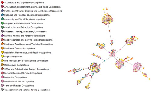
Although commonly used as an outcome-based measure of relatedness, co-location of job classes does not inform us about the type(s) of relatedness between two jobs. In order to empirically unpack the dimensions of relatedness for each pair of job classes, we create other two measures of relatedness: jobs similarity and jobs complementarity.

3.2.2. Jobs similarity

Based on BLS job classes and O*NET’s Work Activities classification scheme, we compute jobs similarity as the frequency of co-occurrences of jobs classes in work activities classes. More specifically, in line with Hasan, Ferguson, and Koning (2015), we first construct a 1 × W vector for each job class, with W being the number of O*NET IWA categories, and then join them to form a binary jobs-IWA matrix (N × W matrix). Then, we apply conditional probabilities for computing jobs similarity measure of relatedness (equivalent to the GeoRel equation, the jobs co-location measure, but based on the jobs-IWA matrix instead). In result, we get a symmetric N × N job classes matrix in which each cell (i, j) contains the skills similarity between job classes i and j. In other words, skills similarity represents, therefore, job classes’ co-occurrences in IWA as the main occupational destination of such skills (e.g. Work Activity w is a highly required skill, more than average in regional labour markets, for both job class a and b).

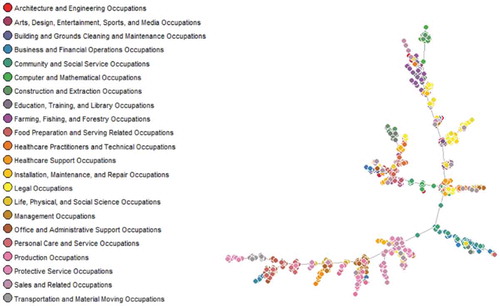
In Figure 2, we present the network graph that illustrates the Similarity dimension of relatedness between all American job classes. As above, we use the Minimum spanning tree network representation algorithm (to show the ‘back bone’ of the network). This network shows a more linear/hierarchical structure than the geographical colocation-based network. Also, as expected, we observe very homogenous agglomerations of job classes (i.e. well-distributed colours – job classes within the same major group of professions).

Figure 2. Similarity dimension of relatedness.

3.2.3. Jobs complementarity

Based on industry clusters’ labour demand, we compute complementarity by looking at which pairs of job classes are jointly required in the same value chain(s). We determine how often two job classes co-occur in the same industry cluster. We first compute each industry cluster’s LQ in each job class, i.e. each cluster employment shares in each job class, compared to the average employment shares of all clusters (same LQ equation we used for jobs co-location measure, but based on the jobs-cluster matrix). Then, we apply conditional probabilities for measuring jobs complementarity (equivalent to GeoRel equation but based on the jobs-cluster matrix). So, we construct a symmetric N × N job classes matrix in which each cell (i, j) contains the jobs complementarity index between job classes i and j.

Finally, in Figure 3, we show the network graph for the Complementarity dimension of relatedness between all American job classes (using Minimum spanning tree algorithm).

Figure 3. Complementarity dimension of relatedness.

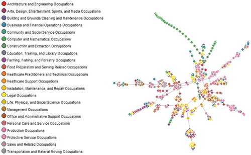
Interestingly, the network built with professional complementarities shows some considerable structural heterogeneity. We can see in this network some level of mixed clustering, i.e. mixed agglomerations in terms of major professional groups (nodes’ colours). Also, a quite linear substructure in the network formed by job classes within the ‘Computer and Mathematical Occupations’. These job classes appear together also in the similarity network. So, they seem to be simultaneously similar in skills and complementary in tasks. Finally, the structure for complementarity also shows some circularity, or ring form.

As we can see already, the three layers for these three measures of relatedness seem to differ substantially in their structure, from more clustered and heterogeneous (i.e. geographically co-located jobs), to more hierarchical and homogeneous (i.e. similar jobs), or to mixed configurations of clustering with hierarchical, centralised with ring form. In other words, the American employment structure seems to show indeed different ‘back bones’ and basis of analysis, depending on the dimension of relatedness we consider in the analysis.

3.2.4. Jobs local synergies

From the three measures of geographical relatedness, complementarity and similarity, we can derive the local synergies dimension of relatedness. Pure geographical relatedness confounds the different forces that make jobs co-occur in the same city. Indeed, jobs may co-locate for reasons of complementarity or similarity, so we cannot tell for sure if local synergies do operate or not. However, local synergies are notoriously difficult to identify. They refer to strong agglomerative forces, but not of the complementarity and the similarity kind. Because some pairs of complementary and/or similar job classes may also have a tendency to co-locate, we need to control for that. We argue that if two job classes have high geographical relatedness but low skills similarity and low industry complementarity, we assume these two job classes show local synergies. So, we deduce the presence of local synergies by identifying pairs of job classes that are most probable to co-locate in cities but do neither show a high degree of jobs complementary nor high jobs similarity.

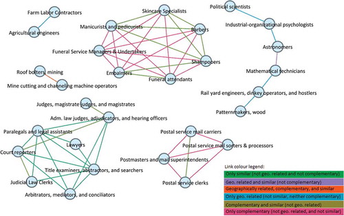
Figure 4 presents the top 50 pairs of related job classes, that is, the 50 highest links of relatedness between occupational specialisations in US cities. Some pairs of jobs, such as ‘roof bolters mining’ and ‘mine cutting and channelling machine operators’, show to be highly related simultaneously due to similarity, complementarity, and they co-locate most often. Other pairs of jobs are highly related mainly due to sharing similar skills, as is the case of ‘lawyers’ and ‘paralegals and legal assistants’, while pairs of jobs like ‘political scientists’ and ‘industrial-organisational psychologists’ are most probably related due to local synergies, as they show to be geographically related and yet, they do not show particularly high similarity or complementarity dimension of relatedness (i.e. they seem to be related in terms of local synergies, and unrelated in complementarities and similarities).

Figure 4. Top 50 pairs of related job classes.

3.3. The job space – a descriptive analysis

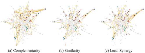
We use the three relatedness measures of geographical relatedness, complementarity, and similarity across jobs to build the Job Space. It is a network-based representation of the US occupational structure (or in other words, of the US national structure of human capital/workforce). Each node of the Job Space stands for a job class, and the links between nodes represent jobs’ relatedness. The Job Space has three different types of links (multiplex network), one for each dimension of relatedness – Complementarity, Similarity, and Local Synergy. And thus, three distinct layers, one for each type of links. For comparison purposes, we show these three layers always with the same nodes in the same position.⁹

Figure 5 shows the US Job Space in 2016. In the first layer, the links show complementarities between job classes. The second layer shows similarities between job classes. And the third layer, local synergies between job classes. We use the Minimum spanning tree network representation algorithm to offer a visualisation in which all job classes are included and connected with the minimum links possible, i.e. N-1 links.

Figure 5. The Job Space in three layers.

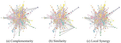
Notice how the configuration of the network varies according to the type of relatedness alone. For instance, Complementarity, and especially Similarity, seem to be somehow expanded in the network, whereas Local Synergy shows much higher concentration in the core of the network, around the nodes with higher degree in the network.

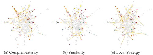
Finally, the three-dimensional Job Space also varies across US cities (MSA), as each city has their specific set of occupational specialisations. In result, for each city, the Job Space shows not only a unique combination of nodes, among their specific set of occupational specialisations, but also a unique combination of links between the existing nodes, and across the three dimensions of relatedness.

For example, Napa (CA) is an MSA with low level of occupational diversification, and mostly concentrated around agriculture and wine industry. Accordingly, as shown in Figure 6, Napa has few occupational specialisations (only 232 nodes), mostly distributed in the periphery of the Job Space, and low level of network density for each relatedness dimension.

Figure 6. The three-dimensional Job Space for Napa, CA.

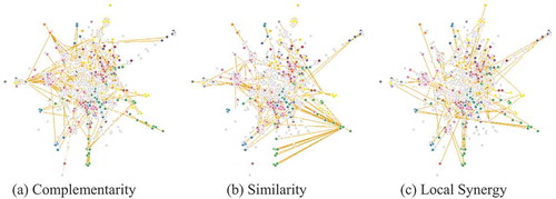
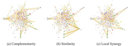
A counter-example is Pittsburgh (PA), which is an MSA with much higher level of economic complexity, highly specialised in manufacturing – especially in the steel industry – but also in software engineering, robotics, energy and environmental design. This is why the Job Space for Pittsburgh (Figure 7) shows a much higher level of diversification (588 occupational specialisations), a higher network density than Napa, and also higher concentration of occupational specialisations in the core of the network.

Figure 7. The three-dimensional Job Space for Pittsburgh, PA.

We also observe that cities with identical levels of diversity might differ in the composition of the three dimensions of relatedness. See for instance Figures 8 and 9 that show the Job Space for the MSAs of Detroit-Dearborn-Livonia and San Jose-Sunnyvale-Santa Clara (which includes Silicon Valley) respectively. They have similar levels of diversity (respectively, 487 and 497 occupational specialisations), but show very different specialisations and also very different combinations of complementarities, similarities, and local synergies. This might indicate that if we analyse related diversification in a city, one should not only look at what new specialisations are added in a city, but also through which dimensions of relatedness this diversification process took place.

Figure 8. The three-dimensional Job Space for Detroit-Dearborn-Livonia, MI.

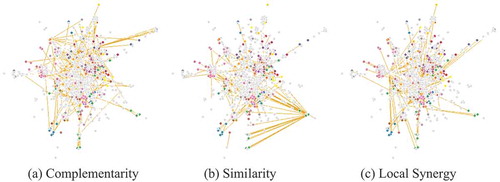
Figure 9. San Jose-Sunnyvale-Santa Clara, CA.

As illustrated in the previous examples of Figures 6 and 7, cities with higher occupational diversification will tend to show higher network density in all dimensions of relatedness. But only cities with especially high levels of diversification in more complex jobs will show especially high density in Local Synergies, as this dimension of relatedness tends to be more concentrated in the core of the network. In Figure 10, we show the Job Space for New York (more precisely, the MSA of New York – Jersey City – White Plains, NY-NJ Metropolitan Division), a more complex and diversified economy, that accordingly shows more central nodes and much higher density of Local Synergies around the core.

Figure 10. The three-dimensional Job Space for New York, NY-NJ.

4. Relatedness dimensions and the renewal of the job-space

Once the job-space is built, we use econometric tools in order to analyse how jobs relatedness affects the renewal of the employment structure of US cities and, in particular, how different dimensions of jobs relatedness (similarity, complementarity, or local synergies) may differently affect that evolution. Starting from 2005, we track yearly changes in the employment structure of each city until 2016, in terms of entry and exit of cities’ occupational specialisations (in other words, entry or exit of a city’s specialisation in a specific strain of human capital), and apply linear probability models to estimate how jobs relatedness affects the entry and exit of job classes in US cities.

So, as we will see in the next sub-session, the entry (exit) of a job class as a new (extinct) occupational specialisation of the city means that the net amount of jobs within that job class increased (decreased), relative to the country’s cities specialisation structure in the previous year, to the point of making it a new (extinct) occupational specialisation in that city.

4.1. Variables and descriptives

We first construct two dummy variables, Entry and Exit. Entry is conventionally computed as equal to one if a job class did not belong to the occupational specialisation portfolio of city c in time t-1, and enters in time t. And Exit is equal to one if a job class did belong to the occupational specialisation portfolio of city c in time t-1, but exits in time t:

$Entr{y}_{c,i,t}=1,\mathrm{i}\mathrm{f}L{Q}_{c,i,t}>1andL{Q}_{c,i,t-1}\le 1$

$Exi{t}_{c,i,t}=1,\mathrm{i}\mathrm{f}L{Q}_{c,i,t}\le 1andL{Q}_{c,i,t-1}>1$

LQ ranks cities level of specialisation in relation to the average level of specialisation of all regions in a year. This means that the position in the ranking of a city may vary from one year to another, not due to changes in that city’s level of specialisation but to changes in other cities’ level of specialisation that affect the average level of specialisation of an economy. So, a job class could change from being a city specialisation t-1 but not any more in t, just because the ranking of specialisation of that job class increased overall in the average economy, not because the share of employees in that city decreased. To exclude such ‘false’ changes in computing Entry and Exit, we made a slight adjustment to the LQ in t .¹⁰ We track the evolution of an occupational specialisation in the city in relation to the pre-existing structure of the city, from t-1 to t, independent of the evolution of the economy’s average specialisation level, which we fix at t-1 when computing LQ in t, as follows:

$Entr{y}_{c,i,t}=1,\mathrm{i}\mathrm{f}L{Q}_{c,i,t,t-1}>1andL{Q}_{c,i,t-1,t-1}\le 1$

$Exi{t}_{c,i,t}=1,\mathrm{i}\mathrm{f}L{Q}_{c,i,t,t-1}\le 1andL{Q}_{c,i,t-1,t-1}>1$

which translates into:

$Entr{y}_{c,i,t}=1,\mathrm{i}\mathrm{f}\frac{\left(\frac{x_{c,i}}{{\sum }_i{x}_{c,i}}\right)t}{\left(\frac{{\sum }_c{x}_{c,i}}{{\sum }_c{\sum }_i{x}_{c,i}}\right)t-1}>1and\frac{\left(\frac{x_{c,i}}{{\sum }_i{x}_{c,i}}\right)t-1}{\left(\frac{{\sum }_c{x}_{c,i}}{{\sum }_c{\sum }_i{x}_{c,i}}\right)t-1}\le 1$

$Exi{t}_{c,i,t}=1,\mathrm{i}\mathrm{f}\frac{\left(\frac{x_{c,i}}{{\sum }_i{x}_{c,i}}\right)t}{\left(\frac{{\sum }_c{x}_{c,i}}{{\sum }_c{\sum }_i{x}_{c,i}}\right)t-1}\le 1and\frac{\left(\frac{x_{c,i}}{{\sum }_i{x}_{c,i}}\right)t-1}{\left(\frac{{\sum }_c{x}_{c,i}}{{\sum }_c{\sum }_i{x}_{c,i}}\right)t-1}>1$

We must account for other variables that may influence Entry and Exit of cities’ occupational specialisations. In our econometric analysis, we use three-way-fixed effects models, with fixed effects for job classes (${\theta }_j$), cities (${\delta }_c$), and years (${\alpha }_t$), accounting for unobservable and invariant specific economic context. In addition, we use six control variables.

Because a bigger and/or more diversified city is more prone to attract new jobs, we compute, for each city in each year, the log of its total employment (City total employment), and the city’s number of occupational specialisations (City diversity). To account for short-term (un)employment growth (especially for years during the crisis), we compute yearly employment growth for cities (City employment growth). Moreover, given global employment trends – like jobs involving more tacit or complex skills having higher and increasing labour demand (Moretti 2012) – we account for labour demand trends by computing the employment growth of each job class (Job employment growth). As a measure of how common/systemic each job class is, we compute the total employment for each job class (Job total employment).

Finally, it is also crucial to control for the specialisation level of a job class. Traditionally, the level of complexity of a job class has somewhat been captured by broad classifications of tasks and skills within job classes (and too broad classifications of job classes), such as the dichotomic degree of routine versus non-routine tasks, or the classification of manual, cognitive, interpersonal, and analytic skills. Such categorisation does not allow to account for the fact that each job class is actually a mix of all those categories. Moreover, for each job class, the specific combination of tasks evolves over time and differs in space, according to its technological context. Also, the more tacit/non-standardised level of a skill, the more difficult to objectively identify it and properly classify it. And therefore, the fewer categories we use to describe the nature of a given job class, the further away we are from capture its specificities.

In order to capture these different dimensions and dynamics, we built a measure of complexity. In particular inspired by the work of Hausmann and Hidalgo (2009) and implemented at the city level by Balland and Rigby (2017), we computed Job Complexity measure using the eigenvector reformulation of the method of reflection. This indicator is based on City diversity (number of occupations a city is specialised in) and Job ubiquity (number of cities that are specialised in a given occupation). Complex jobs are the ones that tend to be found in very few cities (low Job ubiquity) and that are often found in cities that are very diverse (high City diversity).

Following Hidalgo, Klinger, and Barabasi (2007) and Boschma, Balland, and Kogler (2015), we compute geographical relatedness density (GeoRelatedness Density) for each job class j in city c in time t, which represents the relatedness of a new job class specialisation to the set of job classes the city is already specialised in, in a given year. This density measure is derived from the relatedness of job class j to all other job classes i in which the city is specialised in, divided by the sum of relatedness of job class j to all other job classes i in country at time t:

$GeoRelatednessDensit{y}_{j,c,t}=\frac{{\sum }_{i\in c,i\ne j}GeoRe{l}_{j,i}}{{\sum }_{i\ne j}GeoRe{l}_{j,i}}\ast 100$

Likewise, we compute density measures for similarity and for complementarity for each job class j in city c.¹¹ Similarity Density represents the relatedness of a new job class specialisation to the set of job classes the city is already specialised in, in terms of having similar skills. Complementarity Density represents the relatedness of a new job class specialisation to the set of job classes the city is already specialised in, in terms of having complementary skills within the same industry cluster(s).

As explained before, we consider two jobs (city occupational specialisations) to be related in terms of local synergies (i.e. in terms of creating specialised synergies to each other by being close to each other) when they frequently co-locate but show low complementary and low similarity. To calculate Local Synergies Density, we first regress GeoRelatedness Density on Similarity Density and Complementarity Density, using a three-way fixed effects model,¹² as follows:

$GeoRelatednessDensit{y}_{j,c,t-1}=={\beta }_{1}SimilarityDensit{y}_{j,c,t-1}+{\beta }_{2}ComplementarityDensit{y}_{j,c,t-1}+{\theta }_j+{\delta }_c+{\alpha }_t+{\epsilon }_{j,c,t}$

We then save the residuals of the regression, ${\epsilon }_{j,c,t}$, for computing our Local Synergies Density measure. It represents the relatedness of a new occupational specialisation to the set of job classes the city is already specialised in, not in terms of having similar skills or complementary skills with existing job classes, but in terms of sharing the same location.

The panel data includes 11 years (from 2006 to 2016) and 733 job classes in 389 MSA. All our independent variables are lagged by one period (t-1 = [2005 to 2015]), to reduce potential endogeneity.¹³ All our relatedness density variables are centred around the mean for purposes of coefficients’ interpretation. Table 1 shows some descriptive statistics. In Table A1 in the Appendix, we provide descriptives regarding entry and exit for each year for the period 2006–2016.

Table 1. Descriptive statistics.

Statistic	N	Mean	St. Dev.	Min	Max
Entry	2,373,328	0.1	0.2	0.0	1.0
Exit	763,179	0.2	0.4	0.0	1.0
Geo-Relatedness Density	3,136,507	22.6	9.7	1.0	100.0
Complementarity Density	3,136,507	24.4	12.2	0.0	99.8
Similarity Density	3,136,507	24.3	9.7	0.0	93.3
Local Synergies Density	3,136,507	0.0	2.2	−26.2	80.4
City total employment	3,136,507	271,105.4	508,783.7	6,900	6,367,200
Job total employment	3,136,507	143,874.5	339,269.6	30	4,041,050
City employment growth	3,136,507	0.01	0.1	−0.5	2.3
Job employment growth	3,136,507	0.04	0.4	−1.0	25.0
City diversification	3,136,507	178.4	61.5	43.0	385.0
Job Complexity	3,136,507	32.50	19.9	0.0	100

*Number of observations = 733 OCC * 389 MSA * 11 years (from 2006 to 2016) = 3,136,507

Table 2 presents the correlations between all continues variables used in our main analysis, including our four measures of relatedness density and the interaction term between complementarity density and similarity density, that we will use as well in our analysis.

Table 2. Correlation matrix.

	Geo. Relatedness Density	Complementarity Density	Similarity Density	Complementarity Density * Similarity Density	Local Synergies Density	City Total Emp. (ln)	Job Total Emp. (ln)	City Emp. Growth	Job Emp. Growth	City Diversification	Job Complexity
Geo. Relatedness Density	1	0.72	0.83	0.36	0.18	0.65	0.18	−0.04	−0.03	0.81	−0.36
Complementarity Density	0.72	1	0.76	0.43	0.00	0.48	0.11	−0.03	−0.02	0.61	−0.16
Similarity Density	0.83	0.76	1	0.44	−0.00	0.61	0.06	−0.04	−0.01	0.79	−0.07
Complementarity Density * Similarity Density	0.36	0.43	0.44	1	−0.01	0.47	−0.02	−0.01	0.01	0.38	0.05
Local Synergies Density	0.18	0.00	−0.00	−0.01	1	−0.00	0.00	−0.00	0	−0.00	−0.00
City Total Emp. (ln)	0.65	0.48	0.61	0.47	−0.00	1	0.00	−0.01	−0.00	0.64	−0.00
Job Total Emp. (ln)	0.18	0.11	0.06	−0.02	0.00	0.00	1	−0.00	−0.03	0.00	−0.37
City Emp. Growth	−0.04	−0.03	−0.04	−0.01	−0.00	−0.02	−0.00	1	0.03	−0.04	−0.01
Job Emp. Growth	−0.03	−0.02	−0.01	0.02	0.00	−0.00	−0.03	0.03	1	−0.00	0.09
City Diversification	0.81	0.61	0.79	0.38	−0.00	0.64	0.00	−0.04	−0.00	1	0.00
Job Complexity	−0.36	−0.16	−0.07	0.05	−0.00	−0.00	−0.37	−0.01	0.09	0.00	1

4.2. Entry and exit models – only geographical relatedness measure

In the first econometric model, we simply regress Entry of a new occupational specialisation in a city, and Exit of an existing occupational specialisation in a city, on geographical relatedness density (plus controls and fixed effects), as follows:

$Y_{j,c,t}=[Entr{y}_{j,c,t},Exi{t}_{j,c,t}]$

$Y_{j,c,t}={\beta }_{1}GeoRelatednessDensit{y}_{j,c,t-1}+$

$+{\beta }_{2}ln{\left(CityTotalEmp.\right)}_{c,t-1}+{\beta }_{3}ln{\left(JobTotalEmp.\right)}_{j,t-1}+$

$+{\beta }_{4}CityEmp.Growt{h}_{c,t-1}+{\beta }_{5}JobEmp.Growt{h}_{j,t-1}+$

$+{\beta }_{6}CityDiversificatio{n}_{c,t-1}+{\beta }_{7}JobComplexit{y}_{j,t-1}+$

$+{\theta }_j+{\delta }_c+{\alpha }_t+{\epsilon }_{j,c,t}$

with, $\theta$, $\delta$, and $\alpha$being fixed effects, respectively for job classes, cities, and years ($\epsilon$ is the error term).

The results presented in Table 3 show a statistically and economically significant impact of geographical relatedness density on both Entry and Exit. It shows a positive coefficient of 0.021 in the entry model, meaning that when GeoRelatednes Density increases by 10 percentage points, the probability of entry of a new job specialisation in the city increases by 21%. Regarding Exit, the results show a negative impact of relatedness on the probability of a job class exiting a city’s portfolio of occupational specialisations. When GeoRelatednes Density increases by 10 percentage points, the probability of exit of a job class in the city decreases by 33%. All our control variables show to be statistically significant in our Entry models and/or in Exit models. In particular, our variable for Job Complexity seem to foster Entry and prevent Exit of a job class, although with small regression coefficients, and therefore economically not very significant.

Table 3. Entry and exit models – Only geographical measure of relatedness.

	Dependent variable (2006–2016):
	Entry (= 1)	Exit (= 1)
	(1)	(2)
Geo. Relatedness Density	0.021***	−0.033***
	(0.0001)	(0.0003)
City Total Emp. (ln)	0.011***	−0.104***
	(0.003)	(0.009)
Job Total Emp. (ln)	0.005***	−0.078***
	(0.001)	(0.004)
City Emp. Growth	0.036***	−0.020**
	(0.003)	(0.009)
Job Emp. Growth	−0.001	−0.015***
	(0.0004)	(0.005)
City Diversification	−0.003***	0.005***
	(0.00002)	(0.0001)
Job Complexity	0.003***	−0.005***
	(0.00004)	(0.0002)
City fixed effects	Yes	Yes
Job class fixed effects	Yes	Yes
Year fixed effects	Yes	Yes
Observations	2,373,328	763,179
R^2	0.074	0.069
Adjusted R^2	0.074	0.068

The dependent variable entry (exit) equals one if a city c gains (loses) a relative occupational advantage in a given job class j in year t, and equals zero otherwise. All the independent variables are mean-centred and lagged by one year. Period under analysis ranges from 2005 to 2016 (t-1 = [2005–2015]). Coefficients are statistically significant at the ´p < 0.1, * p < 0.05, ** p < 0.01, *** p < 0.001 level. Standard errors in parentheses.

The results so far are in line with the recent literature showing that relatedness seems to play a role in the renewal of the employment structure of US cities, at least when referring to geographical relatedness alone. But given the different reasons for job classes to co-occur, or put differently, we still lack understanding of which dimensions influence the evolution of the employment structure in cities. To test this, instead of geographical relatedness density, next we include in the models our density measures for similarity, complementarity and local synergies.

4.3. Entry and exit models – all dimensions of relatedness

We start by regressing Entry and Exit on each of the three dimensions of relatedness density one at a time. Then, we include them all together, plus an interaction term between Similarity Density and Complementarity Density, to account for pairs of jobs that are simultaneously similar and complementary. The complete models for Entry and Exit are as follows:

$Y_{j,c,t}=[Entr{y}_{j,c,t},Exi{t}_{j,c,t}]$

$\begin{array}{rl}& Y_{j,c,t}={\beta }_{1}ComplementarityDensit{y}_{j,c,t-1}+{\beta }_{2}SimilarityDensit{y}_{j,c,t-1}\\ & +{\beta }_{3}LocalSynergiesDensit{y}_{j,c,t-1}\\ & +{\beta }_{4}SimilarityDensity\ast ComplementarityDensit{y}_{j,c,t-1}\\ & +{\beta }_{5}ln{\left(CityTotalEmp.\right)}_{c,t-1}+{\beta }_{6}ln{\left(JobTotalEmp.\right)}_{j,t-1}\\ & +{\beta }_{7}CityEmp.Growt{h}_{c,t-1}+{\beta }_{8}JobEmp.Growt{h}_{j,t-1}\\ & +{\beta }_{9}CityDiversificatio{n}_{c,t-1}+{\beta }_{10}JobComplexit{y}_{j,t-1}\\ & +{\theta }_j+{\delta }_c+{\alpha }_t+{\epsilon }_{j,c,t}\end{array}$

The results in Tables 4 and 5 show that each dimension of relatedness density, either alone or jointly, has a significant effect on the probability that a city specialises in a new job class or loses an existing job class. The stronger effect on Entry comes from Local Synergies Density, where an increase of 10 percentage points (say, from 25% to 35%) is associated with an 18% increase in the probability of entry (say, from the average of 10% to 11.8% probability of entry). Its effect seems to be even stronger for Exit, with a decrease of 29% on exit probability when Local Synergies Density increases by 10% (say, from the average of 20% to 14.2% probability of exit).

Table 4. Entry models – All dimensions of relatedness density.

		Dependent variable:
		Entry (= 1) | 2006–2016
		(1)	(2)	(3)	(4)
Complementarity Density		0.003***			0.003***
		(0.00002)			(0.00003)
Similarity Density			0.004***		0.004***
			(0.00004)		(0.00005)
Local Synergies Density				0.014***	0.018***
				(0.0001)	(0.0001)
City Total Emp. (ln)		0.018***	0.017***	0.013***	0.012***
		(0.003)	(0.003)	(0.003)	(0.003)
Job Total Emp. (ln)		0.007***	0.007***	0.007***	0.005***
		(0.001)	(0.001)	(0.001)	(0.001)
City Emp. Growth		0.035***	0.034***	0.036***	0.036***
		(0.003)	(0.003)	(0.003)	(0.003)
Job Emp. Growth		0.004***	0.004***	0.001**	−0.0003
		(0.0004)	(0.0004)	(0.0004)	(0.0004)
City Diversification		−0.001***	−0.001***	−0.002***	−0.003***
		(0.00002)	(0.00002)	(0.00002)	(0.00002)
Job Complexity		0.0001*	0.0001**	0.002***	0.003***
		(0.00004)	(0.00004)	(0.00004)	(0.00004)
					0.003***
Complementarity Density * Similarity Density					−0.00001***
					(0.00000)
City fixed effects	Yes		Yes	Yes	Yes
Job class fixed effects	Yes		Yes	Yes	Yes
Year fixed effects	Yes		Yes	Yes	Yes
Observations	2,373,328		2,373,328	2,373,328	2,373,328
R^2	0.063		0.060	0.064	0.077
Adjusted R^2	0.063		0.060	0.064	0.077

The dependent variable entry equals one if a city c gains a new relative occupational advantage in a given job class j in year t, and equals zero otherwise. All the independent variables are mean-centred and lagged by one year. Period under analysis ranges from 2005 to 2016 (t-1 = [2005–2015]). Coefficients are statistically significant at the ´p < 0.1, * p < 0.05, ** p < 0.01, *** p < 0.001 level. Standard errors in parentheses.

Table 5. Exit models – All dimensions of relatedness density.

	Dependent variable:
	Exit (= 1) | 2006–2016
	(1)		(2)	(3)	(4)
Complementarity Density	−0.005***				−0.006***
	(0.0001)				(0.0001)
Similarity Density			−0.007***		−0.007***
			(0.0001)		(0.0001)
Local Synergies Density				−0.018***	−0.029***
				(0.0003)	(0.0003)
City Total Emp. (ln)	−0.106***		−0.110***	−0.104***	−0.102***
	(0.009)		(0.009)	(0.009)	(0.009)
Job Total Emp. (ln)	−0.065***		−0.067***	−0.078***	−0.072***
	(0.004)		(0.004)	(0.004)	(0.004)
City Emp. Growth	−0.027***		−0.027***	−0.021**	−0.024***
	(0.009)		(0.009)	(0.009)	(0.009)
Job Emp. Growth	−0.042***		−0.042***	−0.027***	−0.019***
	(0.005)		(0.005)	(0.005)	(0.005)
City Diversification	0.001***		0.001***	0.002***	0.005***
	(0.0001)		(0.0001)	(0.0001)	(0.0001)
Job Complexity	−0.0002		−0.0003	−0.003***	−0.004***
	(0.0002)		(0.0002)	(0.0002)	(0.0002)
Complementarity Density * Similarity Density					0.0001***
					(0.00000)
City fixed effects		Yes	Yes	Yes	Yes
Job class fixed effects		Yes	Yes	Yes	Yes
Year fixed effects		Yes	Yes	Yes	Yes
Observations		763,179	763,179	763,179	763,179
R^2		0.061	0.056	0.056	0.075
Adjusted R^2		0.059	0.055	0.055	0.074

The dependent variable exit equals one if a city c loses a relative occupational advantage in a given job class j in year t, and equals zero otherwise. All the independent variables are mean-centred and lagged by one year. Period under analysis ranges from 2005 to 2016 (t-1 = [2005–2015]). Coefficients are statistically significant at the ´p < 0.1, * p < 0.05, ** p < 0.01, *** p < 0.001 level. Standard errors in parentheses.

Finally, in Table 6, we repeat the complete models but with standardised variables of relatedness density instead (scaled versions of our previous relatedness density variables), in order to jointly test their explanatory power on Entry and Exit and compare coefficients. We find that an increase of one standard deviation in Local Synergies Density increases the probability of entry of a new job class in the city’s portfolio of job specialisations by 17.8%, and decreases the probability of exit by 27.9%. An increase of one standard deviation in Complementarity Density increases the probability of entry of a new job specialisation by 3.8%, and decreases the probability of exit by 7%. And when Similarity Density increases one standard deviation, the probability of entry increases by 3.6% and exit probability decreases by 6.8%. The only finding not in line with expectation is the effect of the combination of complementarity and similarity: it shows a negative effect on entry and a positive effect on exit, although the effects are not sizable.

Table 6. Entry and exit models – All dimensions of relatedness density (scaled).

	Dependent variable (2006–2016):
	Entry (= 1)	Exit (= 1)
	(1)	(2)
Complementarity Density (sc)	0.038***	−0.070***
	(0.0003)	(0.001)
Similarity Density (sc)	0.036***	−0.068***
	(0.0005)	(0.001)
Local Synergies Density (sc)	0.178***	−0.279***
	(0.001)	(0.003)
City Total Emp. (ln)	0.012***	−0.102***
	(0.003)	(0.009)
Job Total Emp. (ln)	0.005***	−0.072***
	(0.001)	(0.004)
City Emp. Growth	0.036***	−0.024***
	(0.003)	(0.009)
Job Emp. Growth	−0.0003	−0.019***
	(0.0004)	(0.005)
City Diversification	−0.003***	0.005***
	(0.00002)	(0.0001)
Job Complexity	0.003***	−0.004***
	(0.00004)	(0.0002)
Complementary Density (sc) * Similarity Density (sc)	−0.001***	0.009***
	(0.0002)	(0.0005)
City fixed effects	Yes	Yes
Job fixed effects	Yes	Yes
Year fixed effects	Yes	Yes
Observations	2,373,328	763,179
R^2	0.077	0.075
Adjusted R^2	0.077	0.074

The dependent variable entry (exit) equals one if a city c gains (loses) a new relative occupational advantage in a given job class j in year t, and equals zero otherwise. All the independent variables are mean-centred and lagged by one year. Additionally, relatedness density variables are scaled by their SD, for comparison purposes (scaled variables denoted by ‘sc’). Period under analysis ranges from 2005 to 2016 (t-1 = [2005–2015]). Coefficients are statistically significant at the ´p < 0.1, * p < 0.05, ** p < 0.01, *** p < 0.001 level. Standard errors in parentheses.

4.4. Robustness analysis

The novelty of the concepts, overall framework, and methodology introduced in this paper required a vast robustness analysis and dialogue with previous research work and colleague scholars. This paper is also product of such collective learning process. In result, we hereby present some exercises for the robustness of our results.

4.4.1. Control for population density

Despite of controlling for city total employment, cities might still have different levels of population density, related to the distribution of amenities and size effect. To test the robustness of our results, and specially, of the impact of the Local Synergies dimension of relatedness on US cities diversification, we include a measure of population density in addition to city total employment. We use data from the US Census 2010, and therefore we now restrict the analysis to the period of 2005 to 2011 (with t-1 = [2005 to 2010]).

The Table 7 below shows the results for the same models presented in the previous analysis (all Dimensions of Relatedness Density, scaled), now including as well Population Density. These results are very much in line with our previous ones, in terms of coefficients’ signs and values. As such, we chose to keep a larger period of analysis and drop this variable in the main results.

4.4.2. Testing for heterogeneity of impacts in regional diversification

It might be also relevant to test how the role of these different dimensions of relatedness in regional diversification might be heterogeneous according to the task content of each job class. In other words, here we aim to show our variables for each dimension of relatedness might vary according jobs’ level of labour specialisation.

First, we create dummy variable High Preparation Job = 1, if the job class requires high level of preparation for the job (= 0, otherwise), based on O*NET Job Zone (a variable that captures the level of preparation required to perform a certain job class¹⁴). As expected, High Preparation Job seems to be related to our previous variable Job Complexity (see Figure 11), as both aim to capture the complexity of skills and tasks embedded in each job class. High Preparation Job is a direct classification according to workers academic degree, training, and experience. And Job Complexity targets the characteristics of such complex skills/tasks, that show to be rare among cities and concentrated in more diversified cities.

Figure 11. Boxplot of job complexity by level high preparation job.

Accordingly, we then run our models for Entry and Exit (scaled variables of relatedness density), but without Job Complexity, first for High Preparation Job = 1, and second for High Preparation Job = 0. The respective results are shown below in Table 7, Table 8 and in Table 9. Again, our main results seem to be robust to this alternative analysis as well.

Table 7. Entry and exit models (scaled) – controlling for population density – 2006–2011.

	Dependent variable (2006–2011):
	Entry (= 1)	Exit (= 1)
	(1)	(2)
Complementarity Density (sc)	0.035***	−0.066***
	(0.001)	(0.001)
Similarity Density (sc)	0.021***	−0.042***
	(0.001)	(0.002)
Local Synergies Density (sc)	0.102***	−0.163***
	(0.001)	(0.004)
City Total Emp. (ln)	−0.019***	−0.118***
	(0.007)	(0.023)
Job Total Emp. (ln)	−0.005***	−0.060***
	(0.001)	(0.007)
City Emp. Growth	0.024***	0.002
	(0.007)	(0.023)
Job Emp. Growth	−0.003***	−0.030***
	(0.001)	(0.008)
City Diversification	−0.0001***	0.0002***
	(0.00001)	(0.00002)
Job Complexity	0.0002***	−0.0001
	(0.00002)	(0.0001)
Population Density	−0.0002***	0.0004***
	(0.00004)	(0.0001)
Complementary Density (sc) *
Similarity Density (sc)	−0.00004	0.009***
	(0.0002)	(0.0005)
City fixed effects	Yes	Yes
Job fixed effects	Yes	Yes
Year fixed effects	Yes	Yes
Observations	1,092,501	332,451
R^2	0.077	0.073
Adjusted R^2	0.076	0.070

The dependent variable entry (exit) equals one if a city c gains (loses) a new relative occupational advantage in a given job class j in year t, and equals zero otherwise. All the independent variables are mean-centred and lagged by one year. Additionally, relatedness density variables are scaled by their SD, for comparison purposes (scaled variables denoted by ‘sc’). Period under analysis ranges from 2005 to 2011 (t-1 = [2005–2010]). Coefficients are statistically significant at the ´p < 0.1, * p < 0.05, ** p < 0.01, *** p < 0.001 level. Standard errors in parentheses.

Table 8. Entry and exit models (scaled) – Filtering for high preparation required jobs.

	Dependent variable (2006–2016):
	Entry (= 1)	Exit (= 1)
	(1)	(2)
Complementarity Density (sc)	0.039***	−0.065***
	(0.001)	(0.001)
Similarity Density (sc)	0.031***	−0.066***
	(0.001)	(0.003)
Local Synergies Density (sc)	0.136***	−0.250***
	(0.002)	(0.005)
City Total Emp. (ln)	0.007*	−0.106***
	(0.004)	(0.016)
Job Total Emp. (ln)	−0.007***	−0.036***
	(0.001)	(0.007)
City Emp. Growth	0.038***	−0.032*
	(0.004)	(0.017)
Job Emp. Growth	0.0003	−0.016*
	(0.001)	(0.010)
City Diversification	−0.003***	0.005***
	(0.00004)	(0.0001)
Complem. Density (sc) * Similarity Density (sc)	0.001***	0.005***
	(0.0003)	(0.001)
City fixed effects	Yes	Yes
Job fixed effects	Yes	Yes
Year fixed effects	Yes	Yes
Observations	881,066	240,032
R^2	0.074	0.070
Adjusted R^2	0.073	0.068

The dependent variable entry (exit) equals one if a city c gains (loses) a new relative occupational advantage in a given job class j in year t, and equals zero otherwise. All the independent variables are mean-centred and lagged by one year. Additionally, relatedness density variables are scaled by their SD, for comparison purposes (scaled variables denoted by ‘sc’). Period under analysis ranges from 2005 to 2016 (t-1 = [2005–2015]). Coefficients are statistically significant at the ´p < 0.1, * p < 0.05, ** p < 0.01, *** p < 0.001 level. Standard errors in parentheses.

Table 9. Entry and exit models (scaled) – Filtering for low preparation required jobs.

	Dependent variable (2006–2016):
	Entry (= 1)	Exit (= 1)
	(1)	(2)
Complementarity Density (sc)	0.037***	−0.071***
	(0.0004)	(0.001)
Similarity Density (sc)	0.033***	−0.064***
	(0.001)	(0.002)
Local Synergies Density (sc)	0.150***	−0.281***
	(0.001)	(0.003)
City Total Emp. (ln)	0.016***	−0.101***
	(0.004)	(0.011)
Job Total Emp. (ln)	−0.006***	−0.046***
	(0.001)	(0.004)
City Emp. Growth	0.034***	−0.021*
	(0.004)	(0.011)
Job Emp. Growth	−0.005***	−0.013**
	(0.0004)	(0.005)
City Diversification	−0.003***	0.005***
	(0.00003)	(0.0001)
Complem. Density (sc) * Similarity Density (sc)	−0.002***	0.010***
	(0.0003)	(0.001)
City fixed effects	Yes	Yes
Job fixed effects	Yes	Yes
Year fixed effects	Yes	Yes
Observations	1,492,262	523,147
R^2	0.075	0.079
Adjusted R^2	0.075	0.077

The dependent variable entry (exit) equals one if a city c gains (loses) a new relative occupational advantage in a given job class j in year t, and equals zero otherwise. All the independent variables are mean-centred and lagged by one year. Additionally, relatedness density variables are scaled by their SD, for comparison purposes (scaled variables denoted by ‘sc’). Period under analysis ranges from 2005 to 2016 (t-1 = [2005–2015]). Coefficients are statistically significant at the ´p < 0.1, * p < 0.05, ** p < 0.01, *** p < 0.001 level. Standard errors in parentheses.

One could expect, however, the impact of Local Synergies Density to be stronger in fostering Entry and in preventing Exit of a new job class. But Local Synergies Density is a residual measure, i.e. it only reflects relatedness that is not of the similarity neither the complementarity type.¹⁵ So, we would need a direct measure of local synergies to compare its impact on job entry and exit, between high and low level of job complexity.

4.4.3. Alternative model specification: two-way fixed effects for city-year and job-year

Finally, we also tested for alternative model specifications. Here, for instance, we present an alternative specification of the fixed effects considered in our regression. For such, we now run the same exact models as in the main analysis, but with alternative fixed effects. Instead of City, Job, and Year, we use City-Year and Job-Year fixed effects.

The idea is to test whether our variable for the Local Synergies dimension of relatedness might be mainly and merely driven by local effects affecting Entry and Exit of job classes from a city job space. If so, Local Synergies Density should display homogeneous effects across jobs. According to our robustness results (for which we took out the control variables that are now invariant in the data, due to the fixed effects considered here), presented below in Table 10, that does not seem to be the case. The coefficients signs and values seem to maintain its explanatory power on Entry and Exit, and therefore, the dimension of local synergies seems to address indeed more than local effects.

Table 10. Entry and exit models (scaled) – two-way fixed effects: city year and job year.

	Dependent variable (2006–2011):
	Entry (= 1)	Exit (= 1)
	(1)	(2)
Complementarity Density (sc)	0.037***	−0.071***
	(0.0003)	(0.001)
Similarity Density (sc)	0.026***	−0.054***
	(0.0005)	(0.001)
Local Synergies Density (sc)	0.200***	−0.318***
	(0.001)	(0.003)
Complem. Density (sc) * Similarity Density (sc)	−0.0005***	0.010***
	(0.0002)	(0.0005)
City fixed effects	No	No
Job fixed effects	No	No
Year fixed effects	No	No
City-Year fixed effects	Yes	Yes
Job-Year fixed effects	Yes	Yes
Observations	2,373,328	763,179
R^2	0.086	0.095
Adjusted R^2	0.081	0.080

The dependent variable entry (exit) equals one if a city c gains (loses) a new relative occupational advantage in a given job class j in year t, and equals zero otherwise. All the independent variables are mean-centred and lagged by one year. Additionally, relatedness density variables are scaled by their SD, for comparison purposes (scaled variables denoted by ‘sc’). Period under analysis ranges from 2005 to 2016 (t-1 = [2005–2015])). Coefficients are statistically significant at the ´p < 0.1, * p < 0.05, ** p < 0.01, *** p < 0.001 level. Standard errors in parentheses.

We also tested the robustness of our results regarding the construction of the dependent variable, in line with alternative dependent variables in, for example, Bahar, Hausmann, and Hidalgo (2014), Bahar and Rapoport (2018), and Hidalgo, Klinger, and Barabasi (2007). More concretely, we repeated our analysis for:

1. entry = 1 if $L{Q}_t>1$ & $L{Q}_{t-1}\le 1$ & $L{Q}_{t-2}\le 1$ & $L{Q}_{t-3}\le 1$; exit = 1 if $L{Q}_t\le 1$ & $L{Q}_{t-1}>1$ & $L{Q}_{t-2}>1$ & $L{Q}_{t-3}>1$

2. entry = 1 if $L{Q}_{t-1}\le 1$ & $L{Q}_t>1$ & $L{Q}_{t+1}>1$ & $L{Q}_{t+2}>1$; exit = 1 if $L{Q}_{t-1}>1$ & $L{Q}_t\le 1$ & $L{Q}_{t+1}\le 1$ & $L{Q}_{t+2}\le 1$

3. entry = 1 if $L{Q}_t>1$ & $L{Q}_{t-1}\le 0.5$; exit = 1 if $L{Q}_t\le 0.5$ & $L{Q}_{t-1}>1$

4. Location Quotient in t as continuous variable

5. Location Quotient’s absolute growth from t-1 to t as continuous variable.

All these five tests are presented in Tables A2-A5 in the Appendix. They confirm and strengthen the results of our main analysis.

The conduction of this paper generated a panoply of interesting and very pertinent discussions around its key concepts, framework of unpacking relatedness, and implications for policy design. There is of course space for improvement and further investigation of the structural mechanisms driving the geography of jobs in the US. For instance, we choose to only lag our longitudinal variables in one year, i.e. when computing our Relatedness Density variables (for Geographical Relatedness, and Local Synergies, Similarity, and Complementarity dimensions of relatedness) we make them all time-varying (2005–2016), and we lagged them only one year (t-1 = [2005 to 2015]). Partly to maximise the number of years of analysis (classification schemes change more substantially in some years, and for instance, the job class reclassification of 2005 onwards does not allow proper comparison with previous years). But also, in order to intentionally capture the churning of occupational specialisations with changes in relatedness density variables more in the short term. In other words, we account for the relatedness of a new/exiting occupational specialisation to the existing set of occupational specialisations in the city, immediately before that entry/exit occurred (in order to see how much dependent it is on the city existing occupational structure, i.e. in terms of their more or less intricate network of complementarities, similarities, and local synergies).¹⁶

5. Concluding remarks

While many studies have looked at regional diversification into new products (Hidalgo, Klinger, and Barabasi 2007), new industries (Neffke, Henning, and Boschma 2011) or new technologies (Kogler, Rigby, and Tucker 2013; Rigby 2015), this paper has taken an occupational-network approach examining the evolution of job portfolio’s in US cities. The paper replicates the result found in other studies on the evolution of occupational structures in cities (Muneepeerakul et al. 2013; Brachert 2016; Shutters, Muneepeerakul, and Lobo 2016) that cities enter new occupational specialisations that are related to existing ones in the city, and exit existing jobs unrelated to their job portfolio’s. What is new about this paper is that we have unpacked three mechanisms through which the entry and exit of jobs in cities takes place. While previous papers looked at the effect of geographical relatedness only, we unravel three mechanisms through which the effect of geographical relatedness might work because co-location of jobs does not tell us much about the forces that make jobs co-occur in the same city: new local jobs may be related to existing local jobs because they share similar skills or provide complementary tasks, or both, or because they benefit from being co-located.

First, we constructed a job space that represents a network of interdependent job classes that includes the three dimensions through which jobs may be related to each other. In doing so, we can unravel links between pairs of jobs in terms of being similar, being complementary, being both similar and complementary, or in terms of sharing local synergies. Second, we investigated the importance of each of these three job relatedness dimensions for the evolution of jobs in 389 US cities for the period 2005–2016. For this purpose, we introduced a new methodological approach to distinguish between the three relatedness effects.

The main finding is that all three relatedness dimensions (similarity, complementarity and local synergies) increase the chances of entry of a new job in a city on the one hand, and decrease the probability of disappearance of an existing job in a city on the other hand. Moreover, we found the negative effect of relatedness on exits of jobs to be stronger than the positive effect of relatedness on entry of jobs: all three relatedness dimensions seem to prevent exit of jobs in cities more than promoting entry of jobs in cities.

The local synergy density effect shows the largest effect on both entry and exit: this outcome suggests that the stronger local synergies across job classes are, the greater the effect on diversification and the harder to dislocate existing job classes.

The complementarity density effect reflects the tendency of an increasing division of labour in cities which brings higher levels of interdependence between job specialisations (Shutters et al. 2018) where each worker’s productivity depends on whether or not she has access to co-workers with specialised skills and know-how that complement her own (Neffke 2017). The similarity density effect found is in line with the tendency of firms and people to cluster geographically to benefit from a pool of labour with related skills (Neffke and Henning 2013). Similarity seems to prevent exit and promote entry of jobs in cities, but not in combination with complementarity. Although this paper provides an important step to unpack relatedness, it is still far from comprehensive (Boschma 2017). First, while we have started to unravel the geographical density effect (controlling for similarity and complementarity), there is a need to investigate what the local synergies dimension consists of. Second, we need more studies in other countries to shed more systematic light on the importance of the different relatedness dimensions. With longer periods of analysis, one could compute larger lag for the variables, and compare our results with more structural changes in the workforce across time. Third, the three dimensions of relatedness density might play different roles depending on the level of knowledge complexity of activities (Balland and Rigby 2017) and should be employed and tested in studies on regional diversification into new products, industries or technologies, besides new jobs. Fourth, we have to make an effort to include institutions in this framework, because regional diversification might also be affected by institutional requirements that different jobs, industries or technologies have in common (Boschma and Capone 2015). And finally, despite some efforts to minimise issues with endogeneity in our models,¹⁷ we acknowledge we cannot rule out the fact that workers/firms/regions’ demographics might affect the degree of relatedness between them.

Disclosure statement

No potential conflict of interest was reported by the authors.

Notes

¹ publicly available at http://www.bls.gov/oes.

² In our robustness analysis, session 4.4, we further include the variable for population density per city, from the US Census 2010..

³ ‘All Other’ titles represent job classes with a wide range of characteristics, which do not fit into one of the detailed O*NET-SOC occupations.

⁴ publicly available at https://www.onetonline.org.

⁵ O*NET provides classification schemes for Work Activities at three levels of aggregation (41 Generalized Work Activities; 332 Intermediate Work Activities; and finally, 2070 Detailed Work Activities). Intermediate Work Activities is the level of aggregation that provides us better network analysis conditions (enough categories, and that are not too common and not too rare across job classes).

⁶ Here we refer to skills in its broad sense, equivalent to the concept of regional capabilities, commonly used in the evolutionary economic geography literature. It corresponds not to O*NET classification schemes for skills (which refers to a much stricter sense of skills), but to O*NET definition of workers’ competencies (it includes classification schemes for skills in the stricter sense, and also for types of knowledge, abilities, experience and training, etc.).

⁷ BLS aggregates NAICS (four-digit level) into the industry sectors, further used in BLS’s employment projections (https://www.bls.gov/emp/ep_data_input_output_matrix.htm).

⁸ Due to classifications correspondence constrains, we exclude the ‘Private households’ sector (not available in BLS employment data) and further pull together a few industry sectors, ending up with 179 sectors instead of 186. More specifically, we aggregate into one the ‘Crop production’, ‘Animal production and aquaculture’, ‘Forestry’ (including ‘Support Activities for Forestry’), and ‘Fishing, hunting and trapping’. We also aggregate into one the governmental sectors (which corresponds to the 2digits NAICS 92 – Public Administration).

⁹ We keep the coordinates of the nodes and only make the type of links vary from layer to layer. For such, we first scale and aggregate the links of the ‘backbones’ of each dimension of relatedness, i.e. the most representative links of each dimension of relatedness. Then, apply a forced network algorithm to re-arrange the nodes according to their relative proximities. Finally, we save the coordinates of the nodes in this network and use it in the visualisation of the Job Space.

¹⁰ For robustness purposes, we also computed Entry and Exit in its traditional form and run the same models in our analysis. The econometric results are very similar, with coefficients changing only slightly and keeping its statistical and economic significance.

¹¹ Regarding variability of our variables across time: (i) Geographical Relatedness is time-varying, from 2005 to 2016, (ii) the similarity and dimension of relatedness is time invariant by construction (based on IWA classification of ONET’s Content model, last revision, 2014), (iii) we built the complementarity dimension of relatedness as time invariant, in order to reduce endogeneity in the model, because despite of controlling for fixed effects of City and Job in our models, we do not control for Industry classes (a time-variant measure of complementarity dimension would be affected by employment flows between industries over time). Finally, (iv) when computing the respective variables of relatedness density, by construction (because the existing set of occupational specialisations of cities varies along time), they are time-varying, from 2005 to 2016.

¹² R software felm package (https://www.rdocumentation.org/packages/lfe/versions/2.6-2291/topics/felm).

¹³ The variables addressed in this paper are inherently dynamic, co-evolving through time. Identifying causality relationships between relatedness and employment structure renewal is beyond the scope of this study. Our ultimate goal is rather to provide a correlation analysis on the mechanisms of relatedness affecting employment structure renewal.

¹⁴ The O*NET Job Zone variable classifies job classes according to academic degree, related experience, on-the-job training, and certifications, into five categories. We aggregate categories 4 and 5 into ‘high preparation required’ (High Preparation Job = 1), and the other categories into ‘low preparation required’ (High Preparation Job = 0).

¹⁵ as mentioned before, there might be overlapped between dimensions of relatedness for each pair of job classes, for instance, a materials engineer and an aeronautics engineer are similar and also complementary in skills required/tasks performed.

¹⁶ To account for possible endogeneity issues from this option, we compute Entry/Exit in t in relation to the city and country occupational structure in t-1, as discussed in Section 4.1 (i.e. we do not consider Entry and Exit of an occupational specialisation in a city if it is only due to structural changes occurred in other cities, as they affect the national occupational specialisation structure).

¹⁷ Along with lagging relatedness density and our control variables for t-1, we build our dependent variables for t mainly based on the pre-existing set of capabilities of the city (MSA) in relation to the pre-existing set of capabilities of the country, and how it evolved from there, from that initial pre-existing job mix of the country. In other words, we assure that a positive and relevant transformation of a revealed comparative advantage of the city in a certain job (Entry/Exit) in t is relative to the national job mix in t-1, not to the national job mix in t. This assures we are capturing an absolute positive and significant change in the city, and not only by posterior structural changes in other cities in t. So, in our dependent variable, we are specifically capturing the structural changes of city’s job mix that occurred after the ‘screenshot’ of the city job mix in t-1 (relative to the national job mix in t-1). Moreover, we control for employment growth in the city and in the job class previous to Entry/Exit, in the same year as relatedness (t-1). And relatedness in t-1 is actually a ‘product’ of the initial job mix of the city relative to the country in t-1.

Appendices

Table A1. Descriptives of entry and exit for all years 2006–2016 in our main analysis.

Statistic	2006	2007	2008	2009	2010	2011	2012	2013	2014	2015	2016
Entry = 1	15,244	17,217	14,368	14,000	14,279	13,846	13,844	13,795	13,247	13,639	13,209
Entry = 0	201,864	200,372	201,518	201,786	201,079	201,355	201,434	201,401	201,964	201,682	202,185
Entry%	8%	9%	7%	7%	7%	7%	7%	7%	7%	7%	7%
Exit = 1	15,725	15,514	14,268	13,572	14,122	13,923	13,762	13,810	13,357	13,712	13,551
Exit = 0	52,304	52,034	54,983	55,779	55,657	56,013	56,097	56,131	56,569	56,104	56,192
Exit%	30%	30%	26%	24%	25%	25%	25%	25%	24%	24%	24%

Table A2. Alternative dependent variable – Entry and exit models (scaled) with expanded period for pre-change in specialisation (t-3 to t-1).

	Dependent variable (2008–2016):
	Entry (= 1)	Exit (= 1)
	(1)	(2)
Complementarity Density (sc)	0.025***	−0.058***
	(0.0003)	(0.001)
Similarity Density (sc)	0.022***	−0.059***
	(0.0004)	(0.002)
Local Synergies Density (sc)	0.119***	−0.252***
	(0.001)	(0.003)
City Total Emp. (ln)	0.011***	−0.083***
	(0.003)	(0.012)
Job Total Emp. (ln)	0.005***	−0.056***
	(0.001)	(0.005)
City Emp. Growth	0.030***	−0.046***
	(0.003)	(0.011)
Job Emp. Growth	−0.0005	−0.048***
	(0.0004)	(0.008)
City Diversification	−0.002***	0.005***
	(0.00002)	(0.0001)
Job Complexity	0.002***	−0.003***
	(0.00004)	(0.0003)
Complem. Density (sc) * Similarity Density (sc)	−0.0004*	0.006***
	(0.0002)	(0.001)
City fixed effects	Yes	Yes
Job fixed effects	Yes	Yes
Year fixed effects	Yes	Yes
Observations	1,719,967	412,861
R^2	0.055	0.066
Adjusted R^2	0.054	0.063

entry = 1 if LQ > 1 in t and LQ < 1 in t-1, t-2 and t-3

exit = 1 if LQ<1 in t and LQ>1 in t-1, t-2 and t-3

The dependent variable entry (exit) equals one if a city c gains (loses) a new relative occupational advantage in a given job class j in year t, given that it was inexistent (existent) in t-1, in t-2, and in t-3, and equals zero otherwise. All the independent variables are mean-centred and lagged by one year. Additionally, relatedness density variables are scaled by their SD, for comparison purposes (scaled variables denoted by ‘sc’). Period under analysis ranges from 2005 to 2016 (t-3 = [2005–2013]). Coefficients are statistically significant at the ´p < 0.1, * p < 0.05, ** p < 0.01, *** p < 0.001 level. Standard errors in parentheses.

Table A5. Alternative dependent variable – Location quotient levels and location quotient growth models (scaled).

	Dependent variable (2006–2016):
	Location Quotient Levels	Location Quotient Growth
	(1)	(2)
Complementarity Density (sc)	0.655***	0.085***
	(0.005)	(0.007)
Similarity Density (sc)	0.523***	0.030***
	(0.008)	(0.010)
Local Synergies Density (sc)	3.395***	1.011***
	(0.014)	(0.019)
City Total Emp. (ln)	0.036	0.522***
	(0.051)	(0.071)
Job Total Emp. (ln)	−0.116***	1.194***
	(0.013)	(0.028)
City Emp. Growth	0.256***	0.006
	(0.050)	(0.074)
Job Emp. Growth	−0.077***	−4.326***
	(0.007)	(0.043)
City Diversification	−0.048***	−0.012***
	(0.0004)	(0.0005)
Job Complexity	0.051***	0.073***
	(0.001)	(0.001)
Complem. Density (sc) * Similarity Density (sc)	−0.118***	−0.022***
	(0.003)	(0.004)
City fixed effects	Yes	Yes
Job fixed effects	Yes	Yes
Year fixed effects	Yes	Yes
Observations	3,136,507	1,337,115
R^2	0.036	0.138
Adjusted R^2	0.035	0.138

Location Quotient in t as continuous variable

Location Quotient’s absolute growth from t-1 to t as continuous variable

The dependent variable in model (1) is the Location Quotient of city c, in job class j, in year t. The dependent variable in model (2) is the growth of the Location Quotient of city c in job class j, from t-1 to t. All the independent variables are mean-centred and lagged by one year. Additionally, relatedness density variables are scaled by their SD, for comparison purposes (scaled variables denoted by ‘sc’). Period under analysis ranges from 2005 to 2016 (t-1 = [2005–2015]). Coefficients are statistically significant at the ´p < 0.1, * p < 0.05, ** p < 0.01, *** p < 0.001 level. Standard errors in parentheses.

References

- Autor, D. 2010. “The Polarization of Job Opportunities in the U.S. Labor Market: Implications for Employment and Earnings.” Center for American Progress and the Hamilton Project.
- Bahar, D., and H. Rapoport. 2018. “Migration, Knowledge Diffusion and the Comparative Advantage of Nations.” Economic Journal 128 (612): 273–305. doi:10.1111/ecoj.12450.
- Bahar, D., R. Hausmann, and C. A. Hidalgo. 2014. “Neighbors and the Evolution of the Comparative Advantage of Nations: Evidence of International Knowledge Diffusion?” Journal of International Economics 92 (1): 1 111–123. doi:10.1016/j.jinteco.2013.11.001.
- Balland, P. A., and D. Rigby. 2017. “The Geography of Complex Knowledge.” Economic Geography 93 (1): 1–23. doi:10.1080/00130095.2016.1205947.
- Balland, P. A., R. Boschma, J. Crespo, and D. Rigby. 2018. “Smart Specialization Policy in the EU: Relatedness, Knowledge Complexity and Regional Diversification.” Regional Studies, forthcoming. doi:10.1080/00343404.2018.1437900.
- Barbour, E., and A. Markusen. 2007. “Regional Occupational and Industrial Structure: Does the One Imply the Other?” International Regional Science Review 29 (1): 1–19.
- Beaudry, P., D. A. Green, and B. Sand. 2012. “Does Industrial Composition Matter for Wages? a Test of Search and Bargaining Theory.” Econometrica 80 (3): 1063–1104. doi:10.3982/ECTA8659.
- Boschma, R. 2017. “Relatedness as Driver behind Regional Diversification: A Research Agenda.” Regional Studies 51 (3): 351–364. doi:10.1080/00343404.2016.1254767.
- Boschma, R., A. Minondo, and M. Navarro. 2013. “The Emergence of New Industries at the Regional Level in Spain. A Proximity Approach Based on Product-Relatedness.” Economic Geography 89 (1): 29–51. doi:10.1111/j.1944-8287.2012.01170.x.
- Boschma, R., and G. Capone. 2015. “Institutions and Diversification: Related versus Unrelated Diversification in a Varieties of Capitalism Framework.” Research Policy 44: 1902–1914. doi:10.1016/j.respol.2015.06.013.
- Boschma, R., P. A. Balland, and D. Kogler. 2015. “Relatedness and Technological Change in Cities: The Rise and Fall of Technological Knowledge in U.S. Metropolitan Areas from 1981 to 2010.” Industrial and Corporate Change 24: 223–250. doi:10.1093/icc/dtu012.
- Boschma, R. A., and K. Frenken. 2006. “Why Is Economic Geography Not an Evolutionary Science? Towards an Evolutionary Economic Geography.” Journal of Economic Geography 6 (3): 273–302. doi:10.1093/jeg/lbi022.
- Brachert, M. 2016. “The Rise and Fall of Occupational Specializations in German Regions from 1992 to 2010.” Relatedness as driving force of human capital dynamics, working paper.
- Breschi, S., F. Lissoni, and F. Malerba. 2003. “Knowledge-Relatedness in Firm Technological Diversification.” Research Policy 32 (1): 69–87. doi:10.1016/S0048-7333(02)00004-5.
- Delgado, M., M. E. Porter, and S. Stern. 2015. “Clusters and the Great Recession.” draft paper presented at DRUID15, 15-17.
- Duranton, J., and D. Puga. 2003. “Micro-Foundation of Urban Agglomeration Economies.” In Handbook of Regional and Urban Economics Vol. 4 Cities and Geography, edited by V. J. Henderson and J. F. Thisse, 1–21. Amsterdam: Elsevier.
- Eck, N. J. V., and L. Waltman. 2009. “How to Normalize Cooccurrence Data? an Analysis of Some Well‐Known Similarity Measures.” Journal of the American Society for Information Science and Technology 60 (8): 1635–1651. doi:10.1002/asi.21075.
- Essleztbichler, J. 2015. “Relatedness, Industrial Branching and Technological Cohesion in US Metropolitan Areas.” Regional Studies 49 (5): 752–766. doi:10.1080/00343404.2013.806793.
- Feser, E. 2003. “What Regions Do Rather than Make: A Proposed Set of Knowledge-Based Occupation Clusters.” Urban Studies 40 (10): 1937–1958. doi:10.1080/0042098032000116059.
- Florida, R. 2002. “The Economic Geography of Talent.” Annals of the Association of American Geographers 92 (4): 743–755. doi:10.1111/1467-8306.00314.
- Frenken, K., F. Oort, and T. Verburg. 2007. “Related Variety, Unrelated Variety and Regional Economic Growth.” Regional Studies 41 (5): 685–697. doi:10.1080/00343400601120296.
- Gagliardi, L., S. Iammarino, and A. Rodríguez-Pose. 2015. “Offshoring and the Geography of Jobs in Great Britain.” Working paper. CEPR DP10855.
- Gereffi, G., and M. Korzeniewicz, eds. 1994. Commodity Chains and Global Capitalism. Westport, CT: Praeger.
- Hasan, S., J. P. Ferguson, and R. Koning. 2015. “The Lives and Deaths of Jobs: Technical Interdependence and Survival in a Job Structure.” Organization Science, Articles in Advance. Catonsville: Informs. doi:10.1287/orsc.2015.1014.
- Hausmann, R., and C. Hidalgo. 2009. “The Building Blocks of Economic Complexity.” Proceedings of the National Academy of Sciences 106: 10570–10575
- He, C., Q. Guo, and D. Rigby. 2015. “Industry Relatedness, Agglomeration Externalities and Firm Survival in China.” Papers in Evolutionary Economic Geography (PEEG), Utrecht University, Department of Human Geography and Spatial Planning, Group Economic Geography. https://EconPapers.repec.org/RePEc:egu:wpaper:1528
- Hidalgo, C., B. Klinger, and A. Barabasi. 2007. “The Product Space Conditions the Development of Nations.” Science 317 (5837): 482–487. doi:10.1126/science.1144581.
- Kogler, D. F., D. L. Rigby, and I. Tucker. 2013. “Mapping Knowledge Space and Technological Relatedness in U.S. Cities.” European Planning Studies 21 (9): 1374–1391. doi:10.1080/09654313.2012.755832.
- Markusen, A. 2004. “Targeting Occupations in Regional and Community Economic Development.” Journal of the American Planning Association 70 (3): 253–268. doi:10.1080/01944360408976377.
- Markusen, A., and G. Schrock. 2006. “The Distinctive City: Divergent Patterns in Growth, Hierarchy and Specialization.” Urban Studies 43 (8): 1301–1323. doi:10.1080/00420980600776392.
- Markusen, A., G. H. Wassall, D. DeNatale, and R. Cohen. 2008. “Defining the Creative Economy: Industry and Occupational Approaches.” Economic Development Quarterly 22 (1): 24–45. doi:10.1177/0891242407311862.
- Markusen, A., K. Chapple, G. Schrock, D. Yamamoto, and P. Yu. 2001. High-Tech and I-Tech: How Metros Rank and Specialize. Minneapolis, MN: Hubert H. Humphrey Institute of Public Affairs.
- Martin, R., and P. Sunley. 2006. “Path Dependence and Regional Economic Evolution.” Papers in Evolutionary Economic Geography (PEEG) 0606, Utrecht University, Department of Human Geography and Spatial Planning, Group Economic Geography.
- Mehta, A. 2014. “5 Ways to Lessen Inequality as Demand for Labor Decreases Worldwide.” http://www.huffingtonpost.com/aashish-mehta/5-ways-lesson-inequality_b_6215708.html
- Moretti, E. 2012. The New Geography of Jobs. New York: Houghton Miffin Harcourt.
- Moretti, E. 2013. “Real Wage Inequality.” American Economic Journal: Applied Economics 5 (1): 65–103.
- Moretti, E., and P. Kline. 2013. “Local Economic Development, Agglomeration Economies and the Big Push: 100 Years of Evidence from the Tennessee Valley Authority.” Quarterly Journal of Economics 129 (1): 275–331.
- Moretti, M. 2011. “Local Labor Markets.” In Handbook of Labor Economics, Vol. 4, 1237–1313. Boston: Houghton Mifflin Harcourt.
- Muneepeerakul, R., J. Lobo, S. Shutters, A. Gomez-Lievano, and M. Qubbaj. 2013. “Urban Economies and Occupation Space: Can They Get “There” from “Here”?” PLoS ONE 8 (9): e73676. doi:10.1371/journal.pone.0073676.
- Neffke, F. 2017. “Coworker Complementarity”. SWPS 2017-05. Available at SSRN: https://ssrn.com/abstract=2929339or http://dx.doi.org/10.2139/ssrn.2929339.
- Neffke, F., and M. Henning. 2013. “Skill Relatedness and Firm Diversification.” Strategic Management Journal 34 (3): 297–316. doi:10.1002/smj.2013.34.issue-3.
- Neffke, F., M. Henning, and R. Boschma. 2011. “How Do Regions Diversify over Time? Industry Relatedness and the Development of New Growth Paths in Regions.” Economic Geography 87: 237–265. doi:10.1111/ecge.2011.87.issue-3.
- Petralia, S., P. A. Balland, and A. Morrison. 2017. “Climbing the Ladder of Technological Development.” Research Policy 46 (5): 956–969. doi:10.1016/j.respol.2017.03.012.
- Renski, H., J. Koo, and E. Feser. 2007. “Differences in Labor versus Value Chain Industry Clusters: An Empirical Investigation.” Growth and Change 38 (3): 364–395. doi:10.1111/grow.2007.38.issue-3.
- Rigby, D. 2015. “Technological Relatedness and Knowledge Space: Entry and Exit of U.S. Cities from Patent Classes.” Regional Studies 49 (11): 1922–1937. doi:10.1080/00343404.2013.854878.
- Rodriguez, F., and A. Jayadev. 2010. “The Declining Labor Share of Income.” Human Development Reports Research Paper, no. 2010/36.
- Shutters, S., J. Lobo, R. Muneepeerakul, D. Strumsky, C. Mellander, M. Brachert, T. Farinha-Fernandes, and L. Bettencourt. 2018. “Urban Occupational Structures as Information Networks: Scaling of Network Density with Number of Occupations.” working paper.
- Shutters, S., R. Muneepeerakul, and J. Lobo. 2015. “Quantifying Urban Economic Resilience through Labour Force Interdependence.” Palgrave Communications 1: 15010. doi:10.1057/palcomms.2015.10.
- Shutters, S., R. Muneepeerakul, and J. Lobo. 2016. “Constrained Pathways to a Creative Urban Economy.” Urban Studies 53 (16): 3439–3454. doi:10.1177/0042098015616892.
- Steijn, M. P. A. 2018. “Improvement on the Association Strength: Implementing a Probabilistic Measure Based on Combinations without Repetition.” Utrecht Working Paper 1–15. (forthcoming).
- Tanner, A. N. 2014. “Regional Branching Reconsidered: Emergence of the Fuel Cell Industry in European Regions.” Economic Geography 90: 403–427. doi:10.1111/ecge.12055.
- Thompson, W. R., and P. R. Thompson. 1987. “Alternative Paths to the Revival of Industrial Cities.” In The Future of Winter Cities, edited by G. Gappert. Newbury Park, 387–412. CA: Sage.
- Thompson, W. R., and P. R. Thompson. 1985. “From Industries to Occupations: Rethinking Local Economic Development.” Economic Development Commentary 9(3): 12–18.
- US Census Bureau. 2015. “Metropolitan and Micropolitan Statistical Areas”. www.census.gov/population/metro/