Machine learning demand forecasting and supply chain performance

ABSTRACT

In many supply chains, firms staged in upstream of the chain suffer from variance amplification emanating from demand information distortion in a multi-stage supply chain and, consequently, their operation inefficiency. Prior research suggest that employing advanced demand forecasting, such as machine learning, could mitigate the effect and improve the performance; however, it is less known what is the extent and magnitude of savings as tangible supply chain performance outcomes. In this research, hybrid demand forecasting methods grounded on machine learning i.e. ARIMAX and Neural Network is developed. Both time series and explanatory factors are feed into the developed method. The method was applied and evaluated in the context of functional product and a steel manufacturer. The statistically significant supply chain performance improvement differences were found across traditional and ML-based demand forecasting methods. The implications for the theory and practice are also presented.

KEYWORDS:

• Demand forecasting
• machine-learning
• supply chain efficiency

1. Introduction

Forecasting the demand for the products generally hinges on the product characteristics and industry's properties (Kolassa and Siemsen 2016). Functional products characterised by long life cycles, less product variety, stable/predictable demand, low-profit margins, and low inventory risk (Fisher 1997; Lee 2002). Thus, the interaction between the product and industry characteristics determines the nuances of a time series for forecasting the demand. That is, forecasting the demand for a functional product downstream of a supply chain and close to the consumer is possibly less challenging than a functional product's demand forecasting located in upstream of a chain (Syntetos et al. 2016, 2). Steel products can be classified as ‘functional' products (Fisher 1997) with relatively predictable demand if sold towards the end of the chain and close to the consumer. However, due to the location of the demand and the propagation of demand information from the downstream to upstream, the steel-producing firms might experience volatility on their demand and market (Lee, Padmanabhan, and Whang 1997). Apart from four identified sources of demand information distortion as one goes from downstream to upstream (Lee, Padmanabhan, and Whang 1997), the demand forecasting updating is one of the main drivers of supply-demand mismatch and inefficiency. That is, each member of the supply chain observes demand from its downstream customer and uses it as a signal to update its future demand forecast and transmit this distorted demand information to its supplier (Gaur 2013). More sophisticated demand forecasting methods could mitigate the bullwhip effect and improve the supply chain efficiency (Wan and Evers 2011).

To further explore the claim that a more advanced demand forecasting method is expected to improve efficiency, in this research, we develop a hybrid method combining time-series data with leading indicators based on machine-learning algorithms. Subsequently, we examined the magnitude and direction of the effect of the newly developed method as compared to the traditional method. It must be noted that the aim of this research is not to identify the optimum forecasting methods (Makridakis and Hibon 2000; Makridakis, Hyndman, and Petropolous 2020) but to explore the effect magnitude of a hybrid and machine-learning-based method on the firm's performance.

Compared with the traditional demand forecasting methods, the Machine Learning (ML)-based forecasting empowered by predictive analytics has helped the firms to enhance customer engagement, and create more accurate demand forecasts as they expand to new markets or channels (Bohanec, Borštnar, and Robnik-Šilkonja 2017; Chase 2017). ML approaches could better predict the demand since they can handle complex interdependencies between so many causal factors with non-linear relation patterns affecting the demand (Ampazis 2015; Tanaka 2010) and, as a result improving the supply chain performance (Minis and Ampazis 2006).

There exist inconclusive findings on the performance implication of ML methods demand forecasting (Bohanec, Borštnar, and Robnik-Šilkonja 2017; Faraway and Chatfield 1998). For instance, some scholars concluded that traditional or statistical methods like exponential smoothing and Winters exponential smoothing yielded comparable or sometimes better forecast accuracy than Artificial Neural Networks (ANNs) (e.g. Foster, Collopy, and Ungar 1992). In any forecasting effort there are three sources of uncertainty, including model uncertainty, parameter uncertainty and data uncertainty (Petropoulos, Hyndman, and Bergmeir 2018). A possible factor accounting for inconsistency is inability of pure and non-combined approaches to demand forecasting resulting to lack of ability to handle all sources of uncertainties. This inability of forecasting approaches invoked more research by blending various ML techniques and statistical models to establish the hybrid techniques such as Autoregressive Integrated Moving Average (ARIMA) combined with ANNs (Aburto and Weber 2007; Armstrong 1986; Jain and Nag 1997; Kourentzes, Barrow, and Petropoulos 2019). Repeatedly, the evidences were found on superiority of combined forecasting methods in particular blending traditional time series with machine learning approaches (Makridakis, Hyndman, and Petropolous 2020, 21)

In recent years, enormous attention has been paid to using artificial intelligence (AI) and ML to predict the demand (e.g. Aburto and Weber 2007; Carbonneau, Laframboise, and Vahidov 2008; Chase 2017). However, there is scant research evidence on the effectiveness of these methods on improving supply chain performance and accounting for the inconsistency of the effectiveness of ML-based forecasting methods (Makridakis, Hyndman, and Petropolous 2020). Specifically, applying the ML-based method yielded mixed results across homogeneous and heterogenous datasets (Makridakis, Hyndman, and Petropolous 2020, 21). For instance, Carbonneau, Laframboise, and Vahidov (2008) reported superior performance for ML-based methods against traditional ones in a homogenous data context while Makridakis, Spiliotis, and Assimakopoulos (2018) concluded the opposite across heterogenous datasets. For instance, Wen et al. (2017), applying ML methods on extensive homogenous product’s sales data in Amazon, found promising results for ML methods (Ferreira, Lee, and Simchi-Levi 2016). Other cases are in chocolate manufacturing and foundry in which the time series are also homogenous (Carbonneau, Vahidov, and Laframboise 2007, 2008). Another issue peculiar to ML methods is the complexity of the method hindering its adoption (Bohanec, Borštnar, and Robnik-Šilkonja 2017). Apart from the inherent intricacy of these methods, it is unclear how much economic value can be gained by adopting them. More research is needed to moderate initial hype surrounding ML methods and their actual value for the organisations.

For innovative products in which there is limited past historical data and short time for supply chain to react (for instance in fashion products) the application of ML methods was found very useful (Choi et al. 2014; Ferreira, Lee, and Simchi-Levi 2016). There is another contextual condition for using ML methods which is homogeneity/heterogeneity of time series. The strong empirical results were found for effectiveness of ML methods in homogenous datasets (Makridakis, Hyndman, and Petropolous 2020). In present study, the primary intent is to first strengthen previous findings of ML usefulness for homogenous datasets and second provide empirical evidence of effect magnitude of these methods on supply chain performance. In this research, A hybrid ML-based demand forecasting method is developed to address this shortcoming in extant understanding using a homogeneous dataset. By using observational data gathered from a steel manufacturing company, we analyze the effect of the new method on forecast accuracy, inventory turns, and cash-conversion cycle and their interactions as the supply chain performance metrics. The primary research question is the following: ‘ What is the direction and magnitude of the effect of the ML-enabled demand forecasting methods on supply chain performance such as forecast accuracy, inventory turns and cash-conversion cycle?'

Some noteworthy contribution is made in this research: first, a hybrid ML-based method using both time series and leading exogenous indicators is developed. This new method development advances the extant research in using Artificial Intelligence for predicting the product's demand. Second, this research provides substantial empirical evidence on the improvement magnitude in adopting ML-based demand forecasting models. These are significant findings to induce both supply chain scholars and practitioners alike researching and employing ML-methods.

2. Research background

Generally, the ability to understand the demand behaviour and devising an effective method to predict it is noted as a critical organisational capability (Armstrong 1988; Cox 1987, 1989; Fildes and Hastings 1994; Mentzer and Gomes 1994; Wheelwright and Makridakis 1977). A well-developed demand forecasting process yields significant performance benefits. Oliva and Watson (2009) report that doubling inventory turn and 50% reduction in on-hand inventory resulted from improving the demand forecasting process. Similarly, Clarke (2006) documented a 25% reduction in days of inventory for Coca-Cola Inc.

In the last few decades, due to globalisation and the outsourcing/offshoring trend, firms have started to source the products from distant markets across the world, primarily to gain production cost-saving (Christopher and Holweg 2017). This has resulted in a significant increase in the lead times of production/procurement of products. As lead times get long, the demand forecast accuracy tends to be lower, and to mitigate the effects; it has become even crucial for firms to accurately forecast the demands (McCarthy et al. 2006; Moon, Mentzer, and Smith 2003). There are other factors such as time-based competition (Golicic and McCarthy 2002) and product proliferation (Bayus and Putsis Jr 1999; Parker 2002) that contribute to the importance of a more accurate demand forecast.

There exist three underlying principles in demand forecasting (Armstrong 1986; Simchi-Levi and Zhao 2005): 1) forecasting is always wrong, 2) the longer the horizon, the lower the accuracy and 3) the more aggregate the demand, the more accurate the forecast (McCarthy et al. 2006). The ultimate goal of managing the supply chains is to ensure the supply matches the demand (Fisher and Chandra 1994; Sasser 1976). This mismatch occurrence varies contingent upon the type of products in a supply chain, the length of supply chains, and the effectiveness of the forecasting/planning process. In recent years, having access to vast amounts of data and the development of a sophisticated method to exploit the big data have extensively helped to mitigate the risks of mismatches (Armstrong 1986; Boone et al. 2019; Ferreira, Lee, and Simchi-Levi 2016; Sanders and Manrodt 1994). The complexity and multitude of the data and developed engines to process them has enabled the supply chain planners to expand the level of analysis to more granular levels and enhanced the ability to improve the forecasting process outcomes for high frequent as well as low frequent (i.e. intermittent) demand time series (Kolassa and Siemsen 2016). The research and practice evidences have concluded that human judgment and statistical models should be combined and complement each other to improve the forecasting process outcomes (Gaur et al. 2007).

Research on forecasting post-1990s (see, for example, DeRoeck 1991; Mahmoud et al. 1992) explicitly recognised the need to focus on new and emerging trends like e-business, the proliferation of products, and advances in information technology. For example, intending to improve forecasting, companies have increasingly invested in point-of-sale (POS) data collection to get access to the real-time data of demand for each stock keeping unit (SKU) segregated by the location they are observed (Moon, Mentzer, and Smith 2003). Besides collecting a more granular level of data, the methods have also evolved (Mentzer and Kent 1999). The traditional practice of using a single forecasting technique has given way to a combination of techniques with several alternatives being considered simultaneously (Mentzer and Kahn 1997; Mentzer and Schroeter 1993, 1994).

2.1. Demand forecasting for functional products vs. innovative products

According to Fisher (1997) products can be classified into two broad categories: (1) short life cycle, unpredictable demand, higher inventory risk, higher obsolescence cost, and resembling a single replenishment inventory model (i.e. innovative products) and (2) long life span, predictable demand, lower inventory risk, lower obsolescence cost, and resembling a multiple replenishment inventory model (i.e. functional products). Generally, demand forecasting for the innovative product at the SKU level is less dependent on the historical performance of the products (Fisher and Chandra 1994; Moe and Fader 2002), whereas functional products demand forecasting is heavily reliant upon historical demand time series. Because of sensitivity to the time or technology and consequently short life span of innovative products, limited information is available on their demand behaviour, and usually, the forecast should be conducted in a limited amount of time and data in a short-selling season (Choi et al. 2014; Fisher 1997). As a result, demand forecasting, especially at individual SKU level, is very much anchored to qualitative and judgmental forecasting approaches (Gaur et al. 2007; Sanders and Manrodt 2003) or more systematic Delphi methods (Dalkey and Helmer 1963).

Recently, scholars began to develop predictive models addressing the time constrain and limited data in innovative products’ demand (Choi et al. 2014; Ferreira, Lee, and Simchi-Levi 2016; Loureiro, Migués, and da Silva 2018; Sun et al. 2008). For example, Choi et al. (2014) developed a hybrid forecasting model to address the time constrains using extreme machine learning (EML) and high-speed neural network (HSNN); and grey method (GM) to tackle the limitation of historical data points. In a similar vein, for developing demand prediction models in an online fashion retailer, Ferreira, Lee, and Simchi-Levi (2016) used machine learning techniques (i.e. regression trees) to first estimate the lost sales from stock-outs and second, predicting demand for items lacking historical data. The regression tree is also handy in predicting new products’ demand (Ferreira, Lee, and Simchi-Levi 2016; Hastie, Tibshirani, and Friedman 2009).

On the other hand, to predict the demand for ‘functional products’ quantitative models are heavily utilised by firms and little expert's judgment is needed to forecast the product demand (Fisher 1997), however generally judgmental adjustment of all demand forecast is widely used by firms using quantitative methods regardless of product types (Fildes et al. 2009; Moritz, Siemsen, and Kremer 2014). The consumer preference for any product may change over time. Such changes may cause a massive deviation from an observed pattern in the past. Therefore when knowledge of certain events leads one to believe that future demand might not track historical trends, some judgment may be warranted to make adjustments in the models (Meeran et al. 2017). In such cases, a heavy reliance on past data with adjustments based on expert judgment should perform more effectively (Sanders and Manrodt 2003).

Various methods have been used to forecast the demand for steel products as an exemplar of functional products based on the level of demand aggregation and the forecast time horizon. The steel products are positioned all the way upstream of many supply chains, and the demand pattern exhibits an intermittent and or even sometimes lumpy behaviour, i.e. infrequent large aggregated orders (Carbonneau, Laframboise, and Vahidov 2008; Kolassa and Siemsen 2016). Prior research has utilised a combination of time series and exogenous (i.e. leading indicators) factors, particularly environmental sustainability-related indicators. Some of them include macro-economic indicators (e.g. GDP per capita) (Linda 2014; Gao and Wang 2010; Xuan and Yue 2016); Intensity of use which is based on the correlation between the number of materials used to produce goods and services and economic performance; Material Flow Analysis (MFA) and cradle-to-cradle model based on steel life span and incorporating available stock of steel, the production rate of new steel, and disposal, scrap and renewal of used steel (Hu et al. 2010; Muller et al. 2006; Wang and Lin 2015); and steel demand as a function of population, purchasing power and technology (Xuan and Yue 2016). As these streams of research indicate, using the leading indicators along with time series is very common in the steel product's demand forecast. Although the ability to predict those exogenous factors in the intended time horizon forecast and continuation of their relationship with time series in the intended forecast time span remains the biggest hurdles (Makridakis, Hyndman, and Petropolous 2020).

2.2. Supply chain efficiency performance

Environmental uncertainty is one of the main drivers of organisational design and performance (Galbraith 1973). A significant component of environmental uncertainty is demand uncertainty augmenting supply-demand mismatch risk. According to Milgrom and Roberts (1988), there exist two ways of accommodating with demand uncertainty in a production system: (1) inventory buffering (i.e. Make-to-Stock production process) and (2) obtaining customer information and better communication (i.e. Make-to-Order production process and substituting inventory by information). These two mechanisms are substitutes, and the companies by designing/redesigning the production process could determine the differentiation point. They could specify which portion of the production/distribution process should run using inventory and which portion by obtaining information from and communicating with customers (Lee 1996). Other than mechanisms in the supply side to accommodate demand uncertainty, firms could improve their demand forecasting capability to mitigate supply-demand mismatch and improve supply chain efficiency.

Assessing the performance consequences of a capable demand forecast process has been under scrutiny in past research (e.g. Oliva and Watson 2009; Clarke 2006). The performance consequences reflect on the firm's supply chain level of analysis (e.g. Gaur 2013; Lambert 2006; Mackelprang et al. 2014). For example, Gunasekaran and Kobu (2007) suggested various performance metrics for different phases of supply chains, viz. plan, source, make, and deliver. Some of these metrics, which are more reflective of efficiency in the supply chain performance, entail forecasting accuracy, labour efficiency, inventory turns, fill rate, and capacity utilisation (Gaur 2013; McCarthy et al. 2006; Mentzer and Kahn 1995). In addition to these non-financial metrics, some of the financial performance indicators such as production and logistics cost per unit, return on investment, cash conversion cycle is also related to the accuracy of demand's forecast (Gaur 2013; Gunasekaran, Patel, and McGaughey 2004).

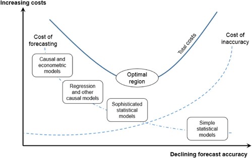
The lack of an effective demand forecast process is very likely to lead to miscoordination across various functions in a firm (Oliva and Watson 2011) and consequently lowering its efficiency. However, the firms must be very cautious of overemphasizing on forecast accuracy. Chambers, Mullick, and Smith (1971) highlight the risk of gold plating (i.e. an attempt to gain more precision than is possibly necessary or possible by using methods such as overfitting the models or adding unnecessary complexity) by the forecasters that offer potentially greater accuracy but may include information that is either non-existent or costly to acquire. The selection of an appropriate forecasting method is critical in a forecasting process and dependents on a variety of factors, i.e. the context of the forecast, the relevance and availability of historical data, the degree of accuracy desirable, the period to be forecast, the cost/ benefit (or value) of the forecast to the company, and the time available for making the analysis.

Figure 1 shows the trade-off between the level of sophistication and cost of accuracy. It can be seen that more complex models deliver higher value (in terms of accuracy) to start with. However, with increasing complexity, the cost also increases and makes the methodology unviable. Evaluating the forecastability of a time series provides useful information on how much effort should be put to enhance the sophistication of forecasting models (Kolassa and Siemsen 2016). There exists an optimal region that is a balance between accuracy achieved by more complexity, viz-a-viz the cost of adding complexity (Fildes and Hastings 1994; Mahmoud et al. 1992). Nowadays, this trade-off between complexity and precision is relaxed to a significant extent due to the advancement of information technology that resulted in less costly access to a considerable amount of data and lowering the cost of developing sophisticated analytical methods (Chase 2017).

Figure 1. Trade-off between inaccuracies in demand forecasting versus the forecasting costs. Adopted from Chambers, Mullick, and Smith (1971).

Inaccurate demand forecast due to long lead times, proliferated offerings, demand information distortion in various industries leads to a detrimental effect in the supply chain dubbed as bullwhip effect (Forrester 1961; Lee, Padmanabhan, and Whang 1997; Wan and Evers 2011). This phenomenon is more prevalent in industries with less seasonal demand, such as the steel industry (Cachon, Randall, and Schmidt 2007), in which there is less motivation for attenuating the demand variability and smoothing the production. In fact, in these industries, due to fixed ordering/set up costs and positively correlated demand, the firms tend to amplify demand variability.

2.3. Artificial intelligence (AI) in demand forecasting

Emulating human brain functionality in computer programs and innovative methods such as deep learning/artificial neural networks has lately gained vast attention in organisational modelling (Chang et al. 2019). Initially there was exaggeration and hype around predictive ability of AI but over time the hype has been moderated by examining the conditions that AI could provide reliable predictive ability (Makridakis, Hyndman, and Petropolous 2020, 20). One of the primary areas of modelling is product demand pattern and forecast inspired by a wide range of various AI models (Bohanec, Borštnar, and Robnik-Šilkonja 2017; Chen and Ou 2011; Choi et al. 2014; Dellino et al. 2018). Traditional demand forecasting approaches can accommodate only a handful of factors that affect the demand to develop a forecast such as trends, seasonality, cyclicality, etc. On the other hand, ML-based forecasting approaches can combine learning algorithms with big data to analyze and account for the sheer number of causal factors with non-linear relation simultaneously (Chase 2017). ML approaches can offer useful tools for both modelling and managing operations in an uncertain environment of the supply chain, especially since the associated techniques are capable of handling complex interdependencies. ML approaches have the ability to learn from the data, make decisions based on the environmental parameters, and then continue to learn from these decisions taken in the past (Goodfellow, Bengio, and Courville 2017).

ML methods have been used in various disciplines, including macro-economics (Franses and Draisma 1997), finance and marketing (Krycha and Wagner 1999; Liu, Singh, and Srinivasan 2016; Qi 1996; Qi and Maddala 1999). Specifically, ML methods have been employed for a wide range of areas in the supply chain, including transportation management, resource allocation and sourcing (Minis and Ampazis 2006), demand forecasting (Aburto and Weber 2007; Carbonneau, Laframboise, and Vahidov 2008; Puchalsky et al. 2018). A few more advanced and hybrid ML techniques have been used to examine the effect of demand forecast inaccuracy on bullwhip effect (Carbonneau, Laframboise, and Vahidov 2008; Gargano and Timmermann 2014; Odonnell et al. 2006).

Incorporating a higher number of explanatory variables such as discounts, promotions, macro-economic factors, price, etc. became possible by advancement in the methods to combine causal regression with time-series models under ANN. For example, Rabelo, Helal, and Lertpattarapong (2004) have used 17 endogenous and exogenous independent variables as an input to the neural network to forecast demand in the short and long term horizons. As another example, Bennett, Stewart, and Lu (2014) have used autoregressive time series models along with other causal factors affecting the demand (i.e. ARIMAX) and neural networks (NN) to predict the energy usage in residential locations.

Lolli et al. (2017) compared the feedforward neural networks with a backpropagation learning scheme with a more straightforward and more efficient learning method called extreme learning machines to predict intermittent demand patterns. Another handy feature of the machine learning algorithm is the property in which they are not required underlying probability distribution. Huber et al. (2019) exploited this property. They used machine learning to provide a reliable solution for retailer's perishable items, in which their ordering decision is based on newsvendor, typically with the assumption of normal distribution.

There exist inconclusive results in utilising ML methods for demand forecasting. For instance, some scholars found that traditional methods like exponential smoothing and Winters exponential smoothing yielded comparable or sometimes better forecast accuracy than ANNs (Dugan, Shriver, and Silhan 1994; Foster, Collopy, and Ungar 1992). Extensive prior research supports the idea of combining several forecasting methods to improve forecast accuracy (Armstrong 2001). This inconsistent evidences invoked more research by blending various ML and statistical techniques to establish hybrid methods such as Autoregressive Integrated Moving Average (ARIMA) combined with ANNs (Aburto and Weber 2007). This hybrid approach of developing the forecasting methods enables the forecaster to account for three types of forecasting model uncertainties i.e. model, parameter and data (Petropoulos, Hyndman, and Bergmeir 2018). This eventually could yield reliable predictions.

2.4. Hypothesis development

According to the forecastability measure computed in Section 3.2 for the company's time-series data, we expect to utilise a more sophisticated forecasting method to improve the forecast accuracy. The ML-based methods developed in this research are indeed more advanced than existing methods at the time the company was using. The extant research on AI and machine-learning demand forecasting models suggest that incorporating non-linear relationships among the variables and allowing the algorithm to learn from the past is expected to improve the predictive ability (Carbonneau, Laframboise, and Vahidov 2008; Wen et al. 2017). Leading indicators are expected to yield better demand forecast accuracy (Makridakis, Hyndman, and Petropolous 2020). A more accurate demand forecast should be translated into improved performance outcomes. Therefore, we posit the following hypothesis:

Hypothesis: Compared with traditional time-series based forecasting approaches, ML-based forecasting approaches could lead to significant improvement in the efficiency of the supply chain.

3. Method

The company's sales and supply chain's performance data is obtained from a multinational steel manufacturing firm. In the past, the company focussed on the ‘building and construction market' segment, which encompasses customised construction steel products. In this segment, the company was able to improve its forecasting and production planning by substituting the inventory with information through communication with the customers (i.e. make-to-order). The manufacturing orders are received in advance, but the challenge lies in meeting quoted lead times to the customers. The availability of raw materials and production capacity when the order is received becomes essential (i.e. a queuing system).

The company expanded its product portfolio into the retail market segment, which is characterised by standardised products. This market segment is the fastest-growing market segment within the company globally, growing at a rate of over 5% by volume year-on-year. It is characterised by many product types that are representative of the entire company product portfolio. As it is common for standard products, the firm uses finished goods inventory buffer to respond to demand changes (i.e. make-to-stock operation) in this market segment. The critical decision for this system is to speculate the demand and produce the steels based on demand forecast. This decision is made in the short-term planning horizon (i.e. 1–3-month period), and demand forecasting has to be reliable at both product family and individual SKU levels. This study is primarily focussed on this market segment. The research design entails two phases: 1) developing hybrid ML-based demand forecasting methods, 2) applying statistical analysis to test the effect of the new methods on performance (Table 1).

Table 1. List of exogenous macro-economic variables.

#	Variable	#	Variable
1	Exports Merchandise	7	Terms of Trade
2	Foreign Reserves,	8	Total Reserves
3	Imports Merchandise,	9	Unemployment Rate
4	Industrial Production,	10	Core CPI,
5	Exchange Rate	11	CPI Price,
6	Stock Markets,

3.1. Observational data

The steel manufacturing company operates in four different market segments, viz. retail, project, manufacturing, and home appliances. The data is collected for one of the business units in all four segments. Figure 2 plots the variation of demand across four market segments at the given business unit. The company currently uses traditional time-series based forecasting techniques. The two traditional forecasting approaches are Holt-Winter and Damped trend methods. The monthly forecast accuracy is monitored, which is equal to {1 – absolute percent error}. Figure 3 shows the forecast accuracy of the two forecasting approaches over five years for the retail market segment. The forecasts are initially generated at the start of every calendar year for a 12-month horizon and updated every month based on the observed demand. Table 2 depicts the uncertainty reflected as the coefficient of variation (CV) of the demand in each market segment and the performance of the existing forecast methods.

Figure 2. Sales volume by market segment in 2012–2017 time span.

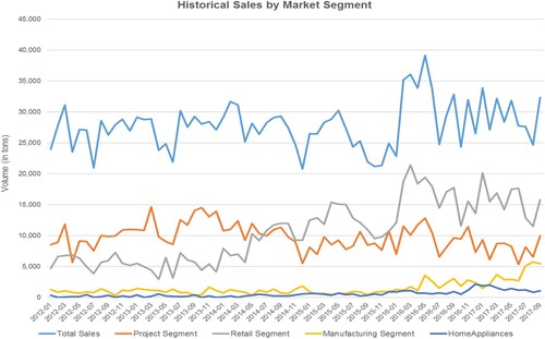
Figure 3. The forecast accuracies for traditional approaches.

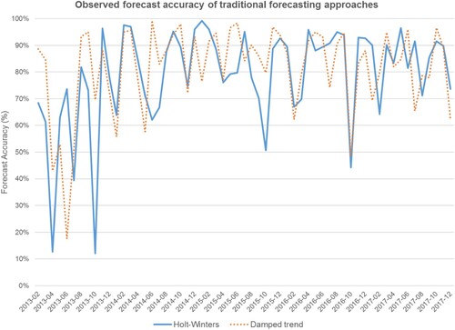
Table 2. Demand uncertainty and existing method forecast error.

	Retail	Project	Manufacturing	Home appliances
Total sales % (by volume)	40%	33%	18%	11%
Coefficient of Variation of demand	46%	22%	78%	89%
Current forecast error (MAPE) in year 2017	32%	25%	35%	71%

According to Table 2, the retail market segment is the largest, with 40 percent of the total volume of sales. Its demand pattern shows significant volatility with CV equal 46% (similar to fast-moving SKUs and their expected demand pattern). Even though the home-appliances and manufacturing market segment had significantly higher CV than retail, at 78% and 89% respectively, but their combined share in the total sales is much less than that of retail alone (i.e. resembles the slow-moving SKUs expected demand pattern). The project market segment is the next biggest in terms of sales volume, but its demand is mainly driven by large construction projects and relatively predictable demand. Since the visibility of such projects is available a few years in advance, the demand for this segment is relatively more stable, and the company has sufficient information to make an accurate forecast and plan for production. This is evident from a lower CV (22%) and lower forecast error (25%) of the project market segment as compared to other segments.

On the other hand, the retail market segment has experienced significant growth in recent years. It is expected to continue to grow, amounting to more than half of the total sales volume. Due to the significant revenue contribution of the retail segment and somewhat unpredictable demand, this segment is the focus of this research. The retail and project segments are less exposed to demand information distortion (e.g. batch ordering) coming from downstream members. Thus we expect the demand time series showing the not-intermittent pattern and can be analyzed using a normal probability distribution. The forecastability of retail demand time series was also examined by computing the following ratio:$Forecastability={\displaystyle \frac{\left(standarddeviationofretaildemandtimeseries\right)}{\left(standarddeviationofretailforecsttimeseriesusingtraditionalmethods\right)}}$If the ratio is larger than 1, it implies there is an avenue to improve the forecast performance using sophisticated methods (Kolassa and Siemsen 2016). Evaluating this ratio using both Holt-Winter and Damped Trends for retail demand time series resulted in 2.6 and 2.8 values, respectively. This implies developing more sophisticated methods to forecast the demand would be beneficial in our setting.

We use following metrics to evaluate supply chain efficiency: inventory turn (IT = Cost of Goods Sold / Average Inventory), forecast accuracy (FA measured by Mean Absolute Percentage Error) and cash-conversion cycle (CCC = days of outstanding receivable + days of outstanding inventory – days of outstanding payable). The first two are operational – oriented measures while the CCC reflects working capital efficiency and financially-oriented barometer. Collectively all three metrics could explain a significant portion of supply chain performance efficiency and sufficiently are adequate to analyze the effect of demand forecasting methods on supply chain efficiency.

We obtained the monthly sales volume panel data for the time frame of 2012–2017 and quarterly basis data for inventory, account receivable, account the payable cost of goods sold, and revenue from Compustat Capital IQ. These data are reported in a consolidated format for publicly listed firms. We converted aggregate data to individual BU basis proportionally to the sales volume for each BU (which is a common tradition in financial forecasting). The monthly data for relevant macro-economic factors are also collected within the same period, primarily from the Global Economic Monitor database provided by the World Bank and other relevant sources. This database compiles various economic indicators, on regional or country basis, such as consumer prices, high-tech market indicators, industrial production and goods, and services trade. We obtained monthly values for 30 macro-economic indicators ranging from the six years (2012–2017). The list of indicators is provided in Table 1.

3.2. Hybrid demand forecasting models

To develop the ML-based forecasting model, we rest on two established models: 1) autoregressive integrated moving average with exogenous variables (ARIMAX) and 2) two-layer feedforward Neural Networks (NN) with backpropagation learning. ARIMAX is similar to the generic ARIMA model with the inclusion of exogenous variables, such as the macro-economic factors. The basic ARIMA (p, d, q) is the generic form of the time series models that are commonly used by econometricians (Box, Jenkins, and Reinsel 2008). It models the time series as autoregressive (AR), integration or differencing order (I), and moving average (MA) components. The parameters of (p, d, q) represent the number of time-lagged in AR, the number of differences as I, and the number of time-lagged forecast errors, respectively. Overall, ARIMA models have performed inferior in demand forecasting against exponential smoothing methods (Makridakis 1993; Makridakis, Hyndman, and Petropolous 2020; Makridakis and Hibon 2000) and both methods grounded on the premise that future demand is a function of the past. However, ARIMAX is based not only on past demand time series but also on leading indicators time series (Box, Jenkins, and Reinsel 2008; Dellino et al. 2018; Makridakis, Hyndman, and Petropolous 2020).

By analyzing autocorrelation function (ACF) and partial autocorrelation functions (PACF) of the time series we observe a significant autocorrelation in AR(1) and AR (3) series while the correlation was not sizable in MA series, thus considering ACF and PACF, the p and q parameters were set at 1 and 0 in the first model and 3 and 0 in the second model (Kolassa and Siemsen 2016). Ali, Boylan, and Syntetos (2015) suggest that if ARIMA models are used for forecasting, a high differencing order is not recommended and most time series can be modelled with no more than two differences (i.e. $d<2$) and AR/MA terms up to order 5 (i.e. $p,q\le 5$). The ARIMAX (1,1,0) model is developed following the rule of minimising the corrected Akaike Information Criterion (AIC). The AIC, in general, is an estimate of lost information. It basically optimises the trade-off between the model goodness-of-fit and the simplicity of the model (Akaike 1973). The ARIMAX (1,1,0) model is specified as:$y_t=\alpha F_t+\text{β}{y}_{t-1}+\gamma \left(y_{t-1}-y_{y-2}\right)+\sum _{j=1}^3{\delta }_j{w}_j+e_t$Where$y_t$ is the demand at time t,$F_t$ is the time-series forecast using Holt-Winter’s method at time t, $\alpha$ is the coefficient for the term $F_t$, $y_{t-1}$is the demand lagged by one time period, $\text{β}$ is the $y_{t-1}$ coefficient, $\gamma$ is the coefficient of the difference term $\left(y_{t-1}-y_{y-2}\right)$, $w_j$ and ${\delta }_j$ denote macro-economic factors and their coefficients respectively and $e_t$ is the error term.

The better fit of higher-order ARIMA demand process in upstream of supply chains is also observed in prior research (Syntetos et al. 2016, 5), and it is largely due to demand variance amplification propagated from downstream to upstream of the chain. Thus, the ARIMAX (3,0,0) model can be specified as below:$y_t=\alpha F_t+\sum _{i=1}^3{\text{β}}_i{y}_{t-i}+\sum _{j=1}^3{\gamma }_j{w}_j+e_t$As one of the deep learning methods, the two-layer feedforward neural network is one of the most popular ML algorithms used in statistical modelling, pattern recognition, etc. (Goodfellow, Bengio, and Courville 2017; Bee-Hua 2000). A feedforward network characterise a mapping $y=f\left(x;\theta \right)$ and learns the value of $\theta$ that provides the best function approximation. The information flows through the function being evaluated at $x$, through the intermediate computation used to define $f$ and finally to the output $y$. The two-layer structure of the network can be specified as $f\left(x\right)=f^2\left(f^1\left(x\right)\right)$. Because the training data doesn’t show the value of other layers than output layer, the other layer is called hidden layers and activation functions should be used to compute the value of hidden layers. The artificial neural networks handle the nonlinear relationship between input variables and the learning occurs as the algorithm compute the gradients of some complicated functions. Back propagation algorithm is used to compute the gradients.

The number of layers represents the depth of the learning network, and the number of neurons in each layer reflects the width of each layer (Goodfellow, Bengio, and Courville 2017). The depth of the learning network was set at a two-layer based on designing multiple experiments and monitoring the validation set's errors (Goodfellow, Bengio, and Courville 2017). This procedure culminated into two-layer yielding better results than one-layer. Increasing the number of layers and depth of learning further would make the optimisation very complicated with a not much higher return. Therefore, we ceased adding more layers and specified the model as two-layer.

The NN model has a similar input variable structure to ARIMAX, including both AR term and exogenous variables, along with the Holt-Winter's forecast. The output of each neuron is determined by the following equations: $v_i=\sum _{h=1}^m{w}_{ih}{x}_h$. Where $v_i$ is the summation of the weights w connecting to the inputs x for neuron i. The weights are computed using backpropagation learning algorithm. The error is calculated at the output and distributed back through the network layers. The final weights are determined based on minimum possible error at the output. There are m inputs with corresponding weights in the previous layer h. If layer h is a hidden layer, each $x_h$is an output of a neuron from the previous layer. Then we have:$Y_i=\sigma \left(v_i\right)={\displaystyle \frac{1}{1+exp\left(-v_{i}a\right)}}$Where $Y_i$ is the output of neuron i, $\sigma \left(v_i\right)$ is the sigmoid activation function and a is the constant which influences the gradient of the function.

In this study, two hidden layers, each with 5 and 2 neurons, respectively, were used to generate the forecast. Two-layer was specified in the model to reflect the more in-depth learning of the algorithm. The number of neurons in the hidden layers is typically within the range of input to output neurons (7 and 1, in this case). In training and testing stages, the 5- and 2-neuron hidden layers structure gave the best forecast accuracy when compared with 6- and 3-neuron hidden layers, 5- and 3-neuron hidden layers, and a single 4-neuron hidden layer models.

3.3. Data generation using developed method

As discussed above, we need to compare the performance of two forecasting approaches concerning supply chain efficiency performance. The data for intended variables need to be generated based on the obtained demand forecast using the new method in order to carry out the performance comparison. The following steps were taken to conduct the comparison:

1. Compiling consolidated financial performance data from Compustat IQ capital within the 2005–2017 time frame,

2. Calculating existing supply chain efficiency metrics using the actual data provided by the company,

3. Generating inventory levels based on new forecast method: the inventory level was generated following the established tradition in financial statement forecasting in which all items of the balance sheet can be generated proportional to the ration of a specific item to the sales volume,

4. Generating supply chain efficiency metrics (i.e. inventory turn, cash-to-cash cycle) using the new forecast method: the same procedure was used as step 3.

4. Results

A correlation analysis was carried out to identify contributing macro-economic factors to the company's sales forecast (Kolassa and Siemsen 2016, 208). Table 3 exhibits the correlation of macro-economic indicators with the sales of the retail market segment. Based on the threshold level of 0.7, following factors are considered since they have a significant correlation (p < .001) with the sales data: (1) Exports Merchandise, (2) Foreign Reserves, (3) Imports Merchandise, (4) Official Exchange rate, (5) Terms of trade, (6) Core CPI. In order to be able to use these factors, their values should be forecasted for the future (Kolassa and Siemsen 2016) and all six indicators are being forecasted regularly by economic research institutions (e.g. Feuerriegel and Gordon 2019). There might be a time lag between these factors to be correlated with sales. The time lag issue is addressed in the model specification.

Table 3. Correlation between macro-economic indicators and historical sales of the retail market segment.

Macro-economic indicator	Correlation coefficient
Exports Merchandise	−0.15
Foreign Reserves	0.74
Imports Merchandise	−0.17
Industrial Production	0.00
Stock Markets	0.45
Terms of Trade	0.84
Total Reserves	0.05
Core CPI	0.86
CPI Price	0.56
Exchange rate	0.24

A linear regression model was built using these six indicators as independent variables and sales values as a dependent. A stepwise estimation procedure (Hair et al. 2013, 184) was utilised, and each variable was included in the model to check if it results in an improvement in R2. This procedure yielded to the inclusion of the following three macro-economic indicators in the model: Foreign reserves, Terms of trade, and Core CPI. To remove multicollinearity, we attempted to include those variables with a lower correlation with other independent variables into the model (Hair et al. 2013). The multicollinearity using the Variance Inflation Factor (VIF) measure was checked, and VIF was at less than four, which indicates no severe issue with multicollinearity.

Foreign reserves of any country are the total value of the foreign currency deposits and bonds held by the central bank and/or monetary authorities of the country. Given that most raw materials are globally traded, having sufficient foreign reserves helps any country to keep the value of its currency more stable. The terms of trade are the relative value of imports of a country in terms of its exports. It is defined as the ratio of the total value of exports to the total value of imports. Higher terms of trade imply that the country can buy more imports per unit of its exports. The core CPI is the consumer price index, excluding energy and food prices. The reason for removing energy and food from the total CPI is because their fluctuation is very high, and it is likely to deviate the index.

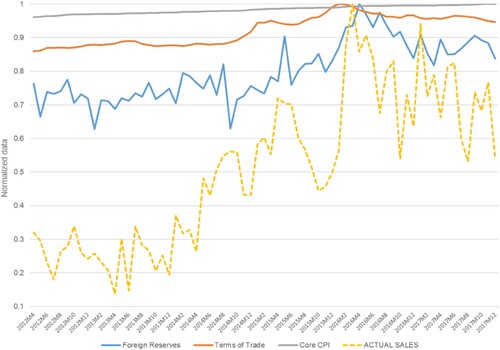
Figure 4 shows the plotting of the three macro-economic factors against historical sales in the retail segment. Considering CPI as a proxy for end-user demand pattern in a steel supply chain and compare it with sales at steel manufacturer reveals variation amplification. The same observation was made in the sales and electronic and automotive products against macro-economic factors (Fine 1998). The CV for CPI is equal to 1.1%, whereas that is 44.6% for steel sales. This observation also verifies our earlier evaluation of the lack of multicollinearity among the variables. Moreover, it confirms the tendency of the steel supply chain to amplify demand variability (Lee, So, and Tang 2000).

Figure 4. The plot of macro-economic factors against historical sales (Normalised data).

4.1. Comparison of traditional and ML-based forecasting methods

Our analysis of historical sales does not indicate strong evidence of demand seasonality and trend in the retail market segment. This indicates stationarity of the time series, thus suitability of ARIMA models to predict it (Chatfield 2007; Kolassa and Siemsen 2016). The two traditional forecasting methods utilised by the company are Holt-Winter's method and the Damped trend method (Acar and Gardner 2012 used the same methods). The dataset was divided into training, testing, and predicting sets to estimate the parameters ARIMAX and ANN models. After obtaining robust parameters in the training dataset and testing them using testing datasets, the parameters were used to predict the demand using ARIMAX and ANN methods.

Since the period of historical sales data was from 2012 to 2016, the forecast was generated monthly for the year 2017. The mean absolute percentage of errors (MAPE) is a ubiquitous measure of point forecast accuracy (Bee-Hua 2000; Kolassa and Siemsen 2016). The forecast was compared with the actual sales data to compute the forecast accuracy (i.e. $Forecastaccuracy\left(\text{\%}\right)=1-MAPE$). Table 4 summarises the results from the traditional forecasting methods.

Table 4. Forecast accuracy results for traditional forecasting methods.

	Forecast Accuracy %
Month	Holt-Winter's method	Damped trend method
1	90.0%	69.3%
2	64.2%	79.7%
3	90.2%	94.9%
4	83.3%	82.0%
5	96.5%	84.7%
6	81.5%	96.0%
7	91.6%	65.5%
8	71.2%	78.6%
9	85.5%	77.9%
10	91.5%	96.6%
11	89.8%	89.1%
12	73.7%	61.9%
Overall Accuracy	84.1%	81.3%

Table 5 provides the estimated coefficients of the ARIMAX models. The forecast accuracy of the ARIMAX (1,1,0) model for the year 2017 is 88.9%. Figure 5 shows the comparison between actual sales and forecast generated using ARIMAX (1,1,0) model. In ARIMAX (3,0,0), the two coefficients of three-time lag variables are positive and statistically significant, and one coefficient is negative, which indicates the presence of bullwhip effect and presence of anti-bullwhip effect respectively (Lee, So, and Tang 2000). However, since two out of three autocorrelations supports the existence of the bullwhip effect, it can be stated that the effect is present in our setting. The forecast accuracy of the ARIMAX (3,0,0) model for the year 2017 is 89.1%. Figure 5 shows the comparison between actual sales and forecast generated using ARIMAX (3,0,0) model. Table 6 summarises the forecast accuracy results for both the ARIMAX models for the year 2017.

Figure 5. Actual sales in retail market segment versus ARIMAX models forecast.

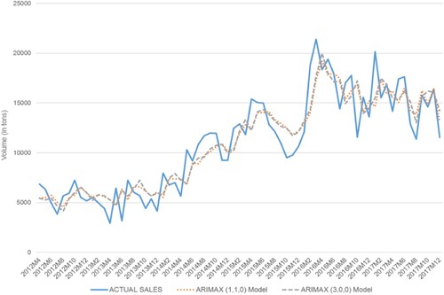
Table 5. ARIMAX coefficient estimates.

ARIMAX (1,1,0)		ARIMAX (3,0,0)
Intercept	−98,263.31	−122058.08
Holt-Winters forecast	−0.0175	0.0397
Demand.Lag1	0.5926	0.4694
Demand.Lag2	-	0.1922
Demand.Lag3	-	−0.1724
Difference term 1	−0.1109	-
Foreign Reserves	164.151	121.8749
Terms of Trade	17,138.205	16396.6854
Core CPI	810.216	1054.8276

Table 6. Comparison of forecast accuracy of ARIMAX (1,1,0) and ARIMAX (3,0,0) forecasting approaches.

	Forecast Accuracy %
Month	ARIMAX (1,1,0)	ARIMAX (3,0,0)
1	62.4%	70.0%
2	89.3%	88.7%
3	94.0%	99.8%
4	87.5%	91.7%
5	84.2%	86.6%
6	93.2%	90.7%
7	90.6%	85.2%
8	82.0%	87.4%
9	97.3%	99.2%
10	98.3%	90.2%
11	99.6%	98.1%
12	88.2%	81.3%
Overall Accuracy	88.9%	89.1%

The result of the Neural Network model is provided in Figure 6. Table 7 summarises the results of the NN forecasting method on forecast accuracy for the year 2017. The Figure 7 shows the comparison between actual sales and forecast generated using NN model. Figure 8 plots the demand prediction of ARIMAX and NN models versus the actual sales. It should be noted that the ARIMAX model can predict the large spikes with one time period lag, as it is evidenced in our result. As is evident in Tables 4, 6, and 7, the ML-based models yielded, on average 5% improvement in forecast accuracy. The 5% improvement in a capital intensive industry such as steel manufacturing can be translated into a significant improvement in supply chain efficiency.

Figure 6. Neural Network model output.

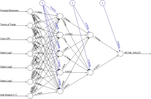
Figure 7. Actual sales in retail market segment versus NN forecast.

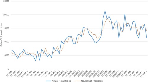
Figure 8. Plot of ARIMAX and NN model against actual sales.

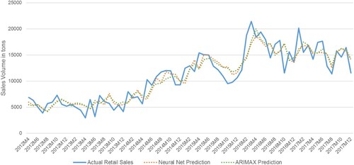
Table 7. Forecast accuracy of NN model for the year 2017.

Forecast Accuracy %
Month	NN with two hidden layers of 5 & 2 neurons
1	75.2%
2	92.6%
3	99.1%
4	93.4%
5	87.2%
6	85.8%
7	84.6%
8	91.0%
9	97.4%
10	90.1%
11	95.2%
12	81.7%
Overall Accuracy	89.4%

4.2. Hypothesis testing

To test the hypothesis on the effect of forecasting approach on supply chain efficiency performance, we specified a regression model as follows: $Y=\alpha +\text{β}X+\epsilon$. Where $Y$ is the supply chain performance, $\alpha$ is a constant, X is a dummy variable coded 0 for traditional forecasting approach and 1 for ML-based forecasting approach, $\text{β}$ is the coefficient of dummy variable $X$, and $\epsilon$ is the i.i.d. error term in predicting the value of Y. To clarify further, $\alpha$ represents the average value of the supply chain performance metric, when traditional time-series based forecasting approach is used; and $\text{β}$ is the mean incremental change in supply chain performance metric when ML based forecasting approach is used. Since we use three performance metrics i.e. forecast accuracy, inventory turn and cash-conversion cycle, three regression models were estimated:

• Model 1: Forecast accuracy (FA): $Y_{FA}={\alpha }_{FA}+{\text{β}}_{FA}X+{\epsilon }_{FA}$

• Model 2: Inventory turns (IT): $Y_{IT}={\alpha }_{IT}+{\text{β}}_{IT}X+{\epsilon }_{IT}$

• Model 3: Cash-conversion cycle (CCC): $Y_{CCC}={\alpha }_{CCC}+{\text{β}}_{CCC}X+{\epsilon }_{CCC}$

If the coefficient of the dummy variable is not zero and statistically significant, there would be empirical evidence that developed machine leaning-based models improve supply chain efficiency performance, and the improvement magnitude is statistically significant. Thus, we tested the following hypothesis:

• H₀: Using the ML-based forecasting approach does not significantly improve the supply chain performance as compared to the traditional forecasting approach. H₀: ${\text{β}}_i$ = 0, for i = FA, IT, CCC.

• H₁: ML-based forecasting approach does significantly improve the supply chain performance as compared to traditional forecasting approach. H₁: ${\text{β}}_i\ne 0$, for i = FA, IT, CCC.

Table 8 summarises the results of the regression models. The dummy variable coefficients (i.e. 0.064, 0.17, −21.6) for all three models are statistically significant at 0.05 and 0.001 levels. The negative value for the CCC model represents a reduction in the cash cycle in terms of the number of days (i.e. CCC reduction is desirable). To further verify the hypothesis test's results also to account for the multicollinearity among the three performance metrics, we employed multivariate analysis of variance (MANOVA). The MANOVA analysis indicates that there is a significant difference between the two forecasting methods on combined performance variables (i.e. P-Value for all four criteria Roy's Greatest Characteristic Root, Wilk's Lambda, Pillai's, Hotelling's Trace were less than 0.01). Thus, both tests support our hypothesis of existence, a significant difference in supply chain efficiency between traditional and ML-based demand forecasting methods. The ML-based demand forecasting methods do improve supply chain performance.

Table 8. Regression coefficient estimates.

	Model 1: Forecast accuracy	Model 2: Inventory turnover	Model 3: Cash conversion cycle
Intercept	0.814	0.12	−19.4
Forecast approach (X)	0.064**	0.17***	−21.6***
Observations	144	144	144
Adjusted R-square	0.091	0.142	0.118

** p < 0.05, *** p < 0.001.

5. Discussion and conclusion

Two research ideas have been reinforced in this research: first, a hybrid method for forecasting the demand combining time series models with leading indicators empowered by machine learning is developed. Second, and more importantly, this research highlights the magnitude of improvement in performance employing advanced forecasting methods. Although the setting of this research and the time series data is not as complicated as prior research to develop a new and optimum forecasting method (e.g. Choi et al. 2014; Ferreira, Lee, and Simchi-Levi 2016; Makridakis 1993), yet it contributes to the ongoing effort of improving the ML methods for demand prediction (Makridakis, Hyndman, and Petropolous 2020). More important than the developed method is the finding of this research on the economic value magnitude of employing these methods for both scholars and practitioners. Using objective pieces of evidence, this research found that significant improvement in supply chain efficiency is expected by utilising ML-based demand forecasting method which is in line with previous research clarifying the value and simplifying these methods for supply chain planners (e.g. Bohanec, Borštnar, and Robnik-Šilkonja 2017; Faraway and Chatfield 1998).

In recent years, much attention has been paid to utilising artificial intelligence to improve data analytics capability in the organisation (e.g. Salinas, Flunkert, and Gasthaus 2017; Wen et al. 2017). In the same line, this research highlighted the value of the ML forecasting approach to improve the supply chain efficiency performance of a supply chain. We combined complementary statistical and ML-based approaches in our analysis to avoid the issue of ML method in vulnerability to excessive variance and the issue of statistical methods in being vulnerable to the bias (Makridakis, Hyndman, and Petropolous 2020). Using developed forecasting methods and panel data from the historical performance of a steel manufacturing firm, we have shown that forecasting methods that are capable of capturing complex relationships of historical data for various variables contributing to demand prediction are performing better than traditional time-series and linear models. This is in line with extant research applying ML method for a large collection of homogenous data (Carbonneau, Laframboise, and Vahidov 2008; Ferreira, Lee, and Simchi-Levi 2016) that ML method is expected to perform well predicting the sales for the homogeneous products. Our findings address the issues of inconsistent research evidence of using AI for demand forecasting by providing more empirical evidence on their effectiveness in homogenous datasets (Dugan, Shriver, and Silhan 1994; Foster, Collopy, and Ungar 1992; Makridakis, Hyndman, and Petropolous 2020). We also responded to the call by Aburto and Weber (2007) to use and test the effect of hybrid models for demand forecasting and its impact on performance outcomes.

We analyzed three performance metrics, one financial and two non-financial. Based on these research findings, it is highlighted that using the ML-based forecasting approach (ARIMAX and NN) could improve both operational and financial metrics. Our results indicate statistically significant improvement in inventory performance. Reducing inventory implies lower storage and facility costs as well as lower transportation expenses without compromising on service level (Acar and Gardner 2012). Specifically in capital intensive industries such as steel manufacturing this assest efficiency is extremely important. The improvement in inventory performance and working capital efficiency resulted from demand prediction improvement is translated into improved return on assets and profitability. Similar results were found by Huber et al. (2019) for perishable items managed by the newsvendor approach that machine learning method outperformed traditional methods and resulted in significant performance improvement for the retailers.

Demand forecasting in this research was conducted at the aggerate level of product family. The research result re-confirms the contribution of macro-economic factors in predicting demand at the aggregate level, and the newly developed model was able to capture and incorporate the complex and non-linear relationship among many variables. To generate the forecasts at lower levels, viz. SKU level, the more accurate aggregate demand forecast, could be translated to more precise demand prediction at individual SKU levels.

The higher level of inefficiency and bullwhip phenomenon is more prevalent in non-seasonal demand and industries (such as steel industry), and they tend to amplify the demand variability more than seasonal demand industries (Cachon, Randall, and Schmidt 2007, 476). An effective demand forecasting process could improve supply chain efficiency to some extent, but more sensible improvement and eliminating the bullwhip effect requires adopting a system view in the supply chain and improve collaboration and communication with supply chain parties (Gaur 2013; Gaur, Giloni, and Seshadri 2005; Lee 1996). However, it is argued that the supply chain integration and ensuing benefits is far from reality (Mackelprang et al. 2014). Then exploiting the data-analytics capability for the firms in the supply chains especially those firms located further from the end consumer help them to achieve favourable outcomes. This research provides further insights in that direction.

Most firms ultimately use judgmental adjustment after using analytical methods to forecast the demand (Boulaksil and Frances 2009; Moritz, Siemsen, and Kremer 2014; Sanders and Manrodt 1994). According to Sanders and Manrodt (2003), 61% of practitioners in their sample who used model-based forecasting methods reported that they ultimately adjust their forecast by their intuition and judgment (Fildes et al. 2009). Thus, it is important to note the value of expert judgment irrespective of the context of forecasting and sophistication of the analytical methods.

Our recommendations for practitioners especially in the context of functional products are two-fold: First, the firms could employ an ML-based approach to forecast the demand for achieving a higher level of accuracy. We showed that the higher level of demand forecast accuracy translates into both improved operational and financial performance outcomes. We also found that the ARIMAX technique was better at predicting the peaks in demand, while neural networks generate more ‘smoothed' prediction with better accuracy. Second, the hybrid approach is advisable, in which several ML techniques could be blended to create a more effective forecasting technique, mainly due to the fact that blended forecast method handles more effectively the model, parameter and data uncertainties (Armstrong 1986). An improved demand forecasting plays a vital role in supply chain planning practice, and increased forecast accuracy will translate directly to better planning in the supply chain (Gaur, Giloni, and Seshadri 2005).

6. Future research and limitations

The result of this research is valid and reliable for contexts in which the product demand highly driven by its past performance. In the industries where the historical performance of the product (e.g. fashion items, fast technology cycle intensive products like smartphones) is less contributing to speculating product demand, our findings do not provide much insight. A similar study could be performed on the effect of an ML-based forecasting approach in a short life cycle (i.e. innovative) product contexts (e.g. Choi et al. 2014) investigate their effect on supply chain performance. The forecasts for such products currently rely very heavily on expert judgments (Gaur et al. 2007). The research could be extended to understand how these expert decisions can be ‘learned' by the ML technique to generate accurate forecasts.

In this research, we used a point forecast accuracy measure evaluating the ML-based methods’ economic value. Apart from point forecast, the ability to handle forecast uncertainty is conceived an unavoidable feature of a forecast performance as the business environment gets more volatile. The predication interval coverage and the width must be at the acceptable range for the forecasting methods to account for uncertainty (Askanazi et al. 2018; Makridakis, Hyndman, and Petropolous 2020). Future studies could expand the findings by incorporating the prediction interval comparison between ML and traditional methods and analyze the supply chain performance implications.

Each of ML and statistical methods are vulnerable to excessive variance and higher bias respectively (Makridakis, Hyndman, and Petropolous 2020). Empirical evidence for economic value of ML method is found in this research and future studies could further evaluate the economic value by combining both ML and statistical/traditional methods. The two approaches are complementary in nature than substitute and there exist lots of overlaps between the two approaches.

A major limitation of this study is the use of single dataset evaluating the forecasting methods. However as elaborated above, the primary intention of this research was to contribute to forecasting process articulation rather than offering an optimum forecasting method. The endeavour to identify the optimum forecasting method requires a different research design which was beyond of the present study’ research objective.

Acknowledgements

This manuscript is developed partially based on the master's degree's thesis by Srivastava, A. and M. de Menezes (2018). A New Approach for Forecasting Demand of Functional Products. Unpublished master's thesis, Malaysia Institute for Supply Chain Innovation, MIT Global SCALE Network.

Disclosure statement

No potential conflict of interest was reported by the author(s).

References

- Aburto, L., and R. Weber. 2007. “Improved Supply Chain Management Based on Hybrid Demand Forecasts.” Applied Soft Computing 7 (1): 136–144.
- Acar, Y., and E. S. Gardner. 2012. “Forecasting Method Selection in a Global Supply Chain.” International Journal of Forecasting 28: 842–848.
- Akaike, H. 1973. “Information Theory and an Extension of the Maximum Likelihood Principle.” In 2nd International Symposium on Information Theory, Tsahkadsor, Armenia, USSR, September 2–8, 1971, edited by B. N. Petrov and F. Csáki, 267–281. Budapest: Akadémiai Kiadó. Republished in Kotz, S., and N. L. Johnson, eds. (1992). Breakthroughs in Statistics. Vol. I, 610–624. New York: Springer-Verlag.
- Ali, Mohammad M., John E. Boylan, and Aris A. Syntetos. 2015. “Forecast Errors and Inventory Performance Under Forecast Information Sharing.” International Journal of Forecasting 28 (4): 830–841.
- Ampazis, N. 2015. “Forecasting Demand in Supply Chain Using Machine Learning Algorithms.” International Journal of Artifical Life Research 5 (1): 56–73.
- Armstrong, J. S. 1986. “Research on Forecasting: A Quarter-Century Review, 1960-1984.” Interfaces 16 (1): 89–10.
- Armstrong, J. S. 1988. “Research Needs in Forecasting.” International Journal of Forecasting 4 (3): 449–465.
- Armstrong, J. S. 2001. “Combining Forecasts.” In Principles of Forecasting, edited by J. Scott Armstrong and Kluwer Aca, 1–19. Norwell, MA: Kluwer.
- Askanazi, R., F. X. Diebold, F. Schorfheide, and M. Shin. 2018. On the Comparison of Interval Forecasts. https://www.sas.upenn.edu/∼fdiebold/papers2/Eval.pdf.
- Bayus, B. L., and W. P. Putsis Jr. 1999. “Product Proliferation: An Empirical Analysis of Product Line Determinants and Market Outcomes.” Marketing Science 18 (2): 137–153.
- Bee-Hua, G. 2000. “Evaluating the Performance of Combining Neural Networks and Genetic Aalgorithms to Forecast Constructuion Demand: The Case of Singapore Residential Sector.” Construction Management and Economics 18: 209–217.
- Bennett, C., R. A. Stewart, and J. Lu. 2014. “Autoregressive with Exogenous Variables and Neural Network Short-Term Load Forecast Models for Residential Low Voltage Distribution Networks.” Energies 7: 2938–2960.
- Bohanec, M., M. K. Borštnar, and M. Robnik-Šilkonja. 2017. “Explaining Machine Learning Models in Sales Prediction.” Experts Systems With Applications 71: 416–428.
- Boone, T., R. Ganeshan, A. Jain, and N. R. Sanders. 2019. “Forecasting Sales in the Supply Chain: Consumer Analythics in a Big Data Era.” Interrnational Journal of Forecsting 35: 170–180.
- Boulaksil, Y., and B. H. Frances. 2009. “Expert's Stated Behaviour.” Interfaces 39 (2): 168–171.
- Box, G. E. P., G. M. Jenkins, and G. C. Reinsel. 2008. Time Series Analysis: Forecasting and Control. 4th ed. Hoboken, NJ: Wiley.
- Cachon, J. P., T. Randall, and G. M. Schmidt. 2007. “In Search of the Bullwhip Effect.” Manufacturing and Service Operations Management 9 (4): 457–479.
- Carbonneau, R., K. Laframboise, and R. M. Vahidov. 2008. “Application of Machine Learning Techniques for Supply Chain Demand Forecasting.” European Journal of Operational Research 184 (3): 1140–1154.
- Carbonneau, R., R. M. Vahidov, and K. Laframboise. 2007. “Machine Leaning-Based Demand Forecasting in Supply Chains.” International Journal of Intelligent Information Technologies 3 (4): 40–57.
- Chambers, J. C., S. K. Mullick, and D. D. Smith. 1971. “How to Choose a Right Forecasting Technique.” Harvard Business Review.
- Chang, S., S. Lee, D. Levinthal, H. E. Posen, P. Puranam, and H. Youn. 2019. “Artificial Intelligence and Next Frontier of Organizational Modelling.” Academy of Management Annula Meeting Proceedings. doi:10.5465/AMBPP.2019.12483symposium.
- Chase, C. W. 2017. “Machine Learning is Changing Demand Forecasting.” Journal of Business Forecasting, 43–45.
- Chatfield, C. 2007. “Confessions of a Pragmatic Forecaster.” Foresight (Los Angeles, CA) 6: 3–9.
- Chen, F. L., and T. Y. Ou. 2011. “Sales Forecasting System Based on Gray Extreme Learning Machine with Taguchi Method in Retail Industry.” Expert Systems With Applications 38: 1336–1345.
- Choi, T. M., H. Chi-Leung, L. Na, N. Sau-Fun, and Y. Yong. 2014. “Fast Fashion Sales Forecasting with Limitted Data and Time.” Decision Support Systems 59: 84–92.
- Christopher, M., and M. Holweg. 2017. “Supply Chain 2.0 Revisited: a Framework for Managing Volatility-Induced Risk in the Supply Chain.” International Journal of Physical Distribution and Logistics Management 47 (1): 2–17.
- Clarke, S. 2006. “Transformation Lessons from Coca-Cola Enterprises Inc.: Managing the Introduction of a Structured Forecast Process.” Foresight: The International Journal of Applied Forecasting 4: 21–25.
- Cox, J. E. 1987. “An Assessment of Books Relevant to Forecasting in Marketing.” International Journal of Forecasting 3: 515–527.
- Cox, J. E. 1989. “Approaches for Improving Salespersons’ Forecasting.” Industrial Marketing Management 18: 307–311.
- Dalkey, N., and O. Helmer. 1963. “An Experimental Application of the Delphi Method to the use of Experts.” Management Science 9 (3): 458–467.
- Dellino, G., T. Laudadio, R. Mari, N. Mastronardi, and C. Meloni. 2018. “A Reliable Decision Support System for Fresh Food Supply Chain Management.” International Journal of Production Research 56 (4): 1458–1485.
- DeRoeck, R. 1991. “Is There a gap Between Forecasting Theory and Practice? A Personal View.” International Journal of Forecasting 7 (1): 1–2.
- Dugan, M. T., K. A. Shriver, and P. Silhan. 1994. “How to Forecast Income Statement Items for Auditing Purposes.” Journal of Business Forecasting Methods and Systems 13: 22–22.
- Faraway, J., and C. Chatfield. 1998. “Time Series Forecasting with Neural Networks: A Comparative Study Using the Airline Data.” Applied Statistics 47: 231–250.
- Ferreira, K. J., B. H. A. Lee, and D. Simchi-Levi. 2016. “Analytics for an Online Retailer: Demand Forecasting and Price Optimization.” Manufacturing and Service Operations Management 16 (1): 69–88.
- Feuerriegel, S., and J. Gordon. 2019. “News-based Forecasts of Macroeconomic Indicators: A Semantic Path Model for Interpretable Predictions.” European Journal of Operational Research 272: 162–175.
- Fildes, R., P. Goodwin, M. Lawrence, and K. Nikolopoulos. 2009. “Effective Forecasting and Judgmental Adjustments: an Empirical Evaluation and Strategies for Improvement in Supply-Chain Planning.” International Journal of Forecasting 25: 3–23.
- Fildes, R., and R. Hastings. 1994. “The Organization and Improvement of Market Forecasting.” Journal of Operational Research Society 45 (1): 1–16.
- Fine, C. H. 1998. Clockspeed: Winning Industry Control in the Age of Temporary Advantage. New York: Basic Books.
- Fisher, M. L. 1997. “What is the Right Supply Chain for Your Product?” Harvard Business Review 97205: 99–129.
- Fisher, M., and P. Chandra. 1994. “Coordination of Production and Distribution Planning.” European Journal of Operational Research 72 (3): 503–517.
- Forrester, J. W. 1961. Industrial Dynamics. Waltham, MA: Pegasus Communications.
- Foster, W., F. Collopy, and L. Ungar. 1992. “Neural Network Forecasting of Short, Noisy Time Series.” Computers & Chemical Engineering 16 (4): 293–297.
- Franses, P. H., and G. Draisma. 1997. “Recognizing Changing Seasonal Patterns Using Artificial Neural Networks.” Journal of Econometrics 81 (1): 273–280.
- Galbraith, J. 1973. Designing Complex Organizations. Reading, MA: Addison-Wesley Publishing Co.
- Gao, X.-R., and A.-J. Wang. 2010. “The Prediction of China's Steel Demand Based on S-Shaped Regularity.” Research Center for Strategy of Global Mineral Resources.
- Gargano, A., and A. Timmermann. 2014. “Forecasting Commodity Price Indexes Using Macroeconomic and Financial Predictors.” International Journal of Forecasting 30 (3): 825–843.
- Gaur, V. 2013. Core Curriculum: Supply Chain Management. Boston, MA: Harvard Business Publishing.
- Gaur, V., A. Giloni, and S. Seshadri. 2005. “Information Sharing in a Supply Chain Under ARMA Demand.” Management Science 51 (6): 961–969.
- Gaur, V., S. Kesavan, A. Raman, and M. L. Fisher. 2007. “Estimating Demand Uncertainty Using Judgmental Forecasting.” Manufacturing and Service Operations Management 9 (4): 480–491.
- Golicic, S. L., and T. M. McCarthy. 2002. “Implementing Collaborative Forecasting to Improve Supply Chain Performance.” International Journal of Physical Distribution and Logistics Management 32 (6): 431–454.
- Goodfellow, I., Y. Bengio, and A. Courville. 2017. Deep Learning. Boston, MA: The MIT Press.
- Gunasekaran, A., and B. Kobu. 2007. “Performance Measures and Metrics in Logistics and Supply Chain Management: a Review of Recent Literature (1995-2004) for Research and Applications.” International Journal of Production Research 45 (12): 2819–2840.
- Gunasekaran, A., C. Patel, and R. E. McGaughey. 2004. “A Framework for Supply Chain Performance Measurement.” International Journal of Production Economics 87: 333–347.
- Hair, J. F., W. C. Black, B. J. Babin, and R. E. Anderson. 2013. Multivariate Data Analysis. 7th ed. Edinburgh: Pearson.
- Hastie, T., R. Tibshirani, and J. Friedman. 2009. The Elements of Statistical Learning: Data Mining, Inference, and Prediction. 2nd ed. New York: Springer.
- Hu, M., S. Pauliuck, T. Wang, G. Huppes, E. V. Voet, and D. B. Muller. 2010. “Iron and Steel in Chinese Residential Buildings: A Dynamic Analysis.” Resources, Conservation and Recycling 54: 591–600.
- Huber, J., S. Müller, M. Fleschemann, and H. Stuckenschmidt. 2019. “A Data Driven Newsvendor Problem: From Data to Decision.” European Journal of Operational Research 278: 904–915.
- Jain, B. A., and B. N. Nag. 1997. “Performance Evaluation of Neural Network Decision Models.” Joumat of Management Information System 14 (2): 201–216.
- Kolassa, S., and E. Siemsen. 2016. Demand Forecasting for Managers. New York: Business Expert Press.
- Kourentzes, N., D. Barrow, and F. Petropoulos. 2019. “Another Look at Forecast Selection and Combination: Evidence From Forecast Pooling.” International Journal of Production Economics 209: 226–235.
- Krycha, K. A., and U. Wagner. 1999. “Applications of Artificial Neural Networks in Management Science: A Survey.” Journal of Retailing and Consumer Services 6 (4): 185–203.
- Lambert, D. M. 2006. Supply Chain Management: Processes, Partnerships and Performance. Sarasota, FL: Supply Chain Management Institute.
- Lee, H. L. 1996. “Effective Inventory and Service Management Through Product and Process Redesign.” Operations Research 4 (1): 151–159.
- Lee, H. L. 2002. “Aligning Supply Chain Strategies with Product Uncertainties.” California Review Management 44: 105–119.
- Lee, H. L., V. Padmanabhan, and S. Whang. 1997. “Information Distortion in a Supply Chain: the Bullwhip Effect.” Management Science 43: 546–558.
- Lee, H. L., K. C. So, and C. S. Tang. 2000. “The Value of Information Sharing in a Two-Level Supply Chain.” Management Science 46: 626–643.
- Linda, W. 2014. “Trends and Developments in Long-Term Steel Demand – The Intensity-of-use Hypothesis Revisited.” Resources Policy 39: 134–143.
- Liu, X., P. V. Singh, and K. Srinivasan. 2016. “A Structured Analysis of Unstructured big Data by Leveraging Cloud Computing.” Marketing Science 35 (3): 363–388.
- Lolli, F., R. Gamberini, A. Regattieri, E. Balugani, T. Gatos, and S. Gucci. 2017. “Single-hidden Layer Neural Networks for Forecasting Intermittent Demand.” International Journal of Production Economics 183: 116–128.
- Loureiro, A. L. D., V. L. Migués, and L. F. M. da Silva. 2018. “Exploring the use of Deep Neural Networks for Sales Forecasting in Fashion Retail.” Decision Support Systems 114: 81–93.
- Mackelprang, A. W., J. L. Robinson, E. Bernardes, and G. S. Webb. 2014. “The Relationship Between Strategic Supply Chain Integration and Performance: A Meta-Analytic Evaluation and Implications for Supply Chain Management Research.” Journal of Business Logistics 35 (1): 71–96.
- Mahmoud, E., R. DeRoeck, R. Brown, and G. Rice. 1992. “Bridging the gap Between Theory and Practice in Forecasting.” International Journal of Forecasting 8 (2): 251–267.
- Makridakis, S. 1993. “The M2-Competition: A Real-Time Judgmentally Based Forecasting Study.” International Journal of Forecasting 9 (1): 5–22.
- Makridakis, S., and M. Hibon. 2000. “The M3-Competition: Results, Conclusions and Implications.” International Journal of Forecasting 16 (4): 451–476.
- Makridakis, S., R. J. Hyndman, and F. Petropolous. 2020. “Forecasting in Social Settings: The State of the art.” International Journal of Forecasting 36: 15–28.
- Makridakis, S., E. Spiliotis, and V. Assimakopoulos. 2018. “Statistical Andmachine Learning Forecasting Methods: Concerns and Ways Forward.” PloS One 13 (3): e0194889.
- McCarthy, T. M., D. F. Davis, S. L. Golicic, and J. T. Mentzer. 2006. “The Evolution of Sales Forecasting Management: A 20-Year Longitudinal Study of Forecasting Practices.” Journal of Forecasting 25: 303–324.
- Meeran, S., S. Jahanbin, P. Goodwin, and J. Q. Nato. 2017. “When do Changes in Consumer Preferences Make Forecasts From Choice-Based Conjoint Models Unreliable?” European Journal of Operational Research 258 (2): 512–524.
- Mentzer, J. T., and R. Gomes. 1994. “Further Extensions of Adaptive Extended Exponential Smoothing and Comparison with the M-Competition.” Journal of the Academy of Marketing Science 22 (4): 372–382.
- Mentzer, J. T., and K. B. Kahn. 1995. “A Framework of Logistics Research.” Journal of Business Logistics 16 (1): 231–248.
- Mentzer, J. T., and K. B. Kahn. 1997. “State of Sales Forecasting Systems in Corporate America.” The Journal of Business Forecasting Methods & Systems 16 (1): 6–13.
- Mentzer, J. T., and J. L. Kent. 1999. “Forecasting Demand in the Longaberger Company.” Marketing Management 8 (2): 46–50.
- Mentzer, J. T., and J. Schroeter. 1993. “Multiple Forecasting System at Brake Parts, Inc.” The Journal of Business Forecasting Methods & Systems 12 (3): 5–21.
- Mentzer, J. T., and J. Schroeter. 1994. “Integrating Logistics Forecasting Techniques, Systems and Administration: the Multiple Forecasting System.” Journal of Business Logistics 15 (2): 205–225.
- Milgrom, P., and J. Roberts. 1988. “Communication and Inventory as Substitutes in Organizing Production.” Scandinavian Journal of Economics 90 (3): 275–289.
- Minis, I., and N. Ampazis. 2006. “Applications of Neural Networks in Supply Chain Management.” Handbook of Research on Nature Inspired Computing for Economics and Management 2.
- Moe, W. W., and P. S. Fader. 2002. “Using Advance Purchase Orders to Forecast New Product Sales.” Marketing Science 21 (3): 347–364.
- Moon, M. A., J. T. Mentzer, and C. D. Smith. 2003. “Conducting a Sales Forecasting Audit.” International Journal of Forecasting 19 (1): 5–25.
- Moritz, B., E. Siemsen, and M. Kremer. 2014. “Judgmental Forecasting: Cognitive Reflection and Decision Speed.” Production and Operations Management 23 (7): 1146–1160.
- Muller, D. B., T. Wang, B. Duval, and T. E. Graedel. 2006. “Exploring the Engine of Anthropogenic Iron Cycles.” Proceedings of the National Academy of Sciences of the United States of America 103: 16111–16116.
- Odonnell, T., L. Maguire, R. McIvor, and P. Humphreys. 2006. “Minimizing the Bullwhip Effect in a Supply Chain Using Genetic Algorithms.” International Journal of Production Research 44 (8): 1523–1543.
- Oliva, R., and N. H. Watson. 2009. “Managing Functional Biases in Organizational Forecasts: A Case Study of Consensus Forecasting in Supply Chain Planning.” Production and Operations Management 18 (2): 138–151.
- Oliva, R., and N. H. Watson. 2011. “Cross-Functional Alignment in Supply Chain Planning: A Case Study of Sales & Operations Planning.” Journal of Operations Management 29 (5): 434–448.
- Parker, K. 2002. “Events Happen, but Demand is Always.” Manufacturing Business Technology 20 (2): 40–43.
- Petropoulos, F., R. J. Hyndman, and C. Bergmeir. 2018. “Exploring the Sources of Uncertainty: why Does Bagging for Time Series Forecasting Work?” European Journal of Operational Research 268 (2): 545–554.
- Puchalsky, W., G. T. Ribeiro, C. P. da Veiga, R. Z. Freire, and L. dos Santos Coelho. 2018. “Agribusiness Time Series Forecasting Using Wavelet Neural Networks and Metaheuristic Optimization: An Analysis of the Soybean Sack Price and Perishable Products Demand.” International Journal of Production Economics 203: 174–189.
- Qi, M. 1996. “Financial Applications of Artifical Neural Networks.” Handbook of Statistics 14: 529–552.
- Qi, M., and G. S. Maddala. 1999. “Economic Factors and the Stock Market: A new Perspective.” Journal of Forecasting 18 (3): 151–166.
- Rabelo, L., M. Helal, and C. Lertpattarapong. 2004. “Analysis of Supply Chains Using System Dynamics, Neural Nets, and Eigenvalues.” Proceedings of the 36th Winter Simulation Conference.
- Salinas, D., V. Flunkert, and J. Gasthaus. 2017. “DeepAR: Probabilistic Forecasting with Autoregressive Recurrent Networks.” arXiv Preprint ArXiv 1704: 04110.
- Sanders, N. R., and K. B. Manrodt. 1994. “Forecasting Practices in US Corporations: Survey Results.” Interfaces 24 (2): 92–100.
- Sanders, N. R., and K. B. Manrodt. 2003. “Forecasting Software in Practice: Use, Satisfaction, and Performance.” Interfaces 33 (5): 90–93.
- Sasser, W. E. 1976. “Match Supply and Demand in the Service Industries.” Harvard Business Review 54 (6): 133–140.
- Simchi-Levi, D., and Y. Zhao. 2005. “Safety Stock Positioning in Supply Chains with Stochastic Lead Times.” Manufacturing & Service Operations Management 7: 295–318.
- Sun, Z. L., T. M. Choi, K. F. Au, and Y. Yu. 2008. “Sales Forecasting Using Extreme Learning Machine with Applications in Fashion Retailing.” Decision Support Systems 46: 411–419.
- Syntetos, A. A., Z. Babai, J. E. Boylan, S. Kolassa, and K. Nikolopoulos. 2016. “Supply Chain Forecasting: Theory, Practice, their Gap and the Future.” European Journal of Operational Research 252 (1): 1–26.
- Tanaka, K. 2010. “A Sales Forecasting Model for New-Released and Nonlinear Sales Trend Products.” Expert Systems with Applications 37: 7387–7393.
- Wan, X., and P. T. Evers. 2011. “Supply Chain Networks With Multiple Retailers: A Test of the Emerging Theory on Inventories, Stockouts, and Bullwhips.” Journal of Business Logistics 32 (1): 27–39.
- Wang, X., and B. Lin. 2015. “Carbon Emissions From Energy Intensive Industry in China: Evidence From the Iron & Steel Industry.” Renewable and Sustainable Energy Reviews 47 (C): 746–754.
- Wen, R., K. Torkkola, B. Narayanaswamy, and D. Madeka. 2017. “A Multi-Horizon Quantile Recurrent Forecaster.” arXiv Preprint ArXiv 1711: 11053.
- Wheelwright, S. C., and S. G. Makridakis. 1977. Forecasting Methods for Management. New York: Wiley.
- Xuan, Y., and Q. Yue. 2016. “Forecast of Steel Demand and the Availability of Depreciated Steel Scrap in China.” Resources Conservation and Recycling 109: 1–12.