Neural net versus classical models for the detection and localization of leaks in pipelines

Abstract

Four models of a pipeline are compared in the paper: a nonlinear distributed-parameter model, a linear distributed-parameter model, a simplified lumped-parameter model and an extended neural-net-based model. The transcendental transfer function of the linearized model is obtained by a Laplace transformation and corresponding initial and boundary conditions. The lumped-parameter model is obtained by a Taylor series extension of the transencdental transfer function. Based on the experience of linear models the structure of the neural net model, as an addendum to the nonlinear distributed-parameter model, is obtained. All four models are tested on a real pipeline data with an artificially generated leak.

Keywords:

• Environmental and safety systems
• Fault and uncertainty modelling in dynamical systems
• Process supervision
• Neural nets

1. Introduction

Many fluids transported by pipelines are in some sense dangerous. It is therefore often necessary to install leak detection (and locating) systems (LDSs), in particular because of legal regulations. Examples are as follows:

1. Code for Federal Regulations Title 49, Part 195 (USA);

2. American Petroleum Institute (API) 1130, 2nd edition (USA);

3. Technical Rules for Pipelines (Germany).

Different methods for leak detection and location are available, for example balancing systems (line balance and volume balance) and real-time transient model (RTTM) systems 1,2. API 1130 defines RTTM systems as LDSs based on algorithmic procedures for calculating the transient fluid mechanical behaviour of the pipeline in real time. Such systems can be treated as technical fault diagnosis systems 3, leading to extended real-time transient model (E-RTTM) systems, which form an online pattern recognition scheme containing feature generation using mathematical models and (statistical) classification algorithms 2.

RRTM and E-RTTM LDSs are perhaps the most sophisticated systems for leak detection and location, but there are still unsolved problems.

1. Only models for single-phase liquid and gas flow are sufficiently exact; models for multiple-phase flow are available, but often too complex or too inaccurate.

2. Many crude oil pipelines are operated using drag-reducing agents (DRAs), which influence the static and transient behaviour of the pipeline significantly. Complete models for DRAs are not yet available.

3. Unknown factors such as sensor offsets or sensor dynamics often degrade LDS performance by falsifying the transient calculation.

4. Unmeasurable variables and parameters have an impact on the static and dynamic pipeline behaviour without the possibility of using analytical models for compensating these effects.

Neural nets, which imitate human ‘hardware’, that is the neurons, will be used in this paper as a mathematical tool to model a nonlinear system, namely the pipeline. This paper is concerned with a model-based RTTM approach, with the use of a mathematical model description of a pipeline in the form of a pipeline observer using classical models and/or neural nets. In the case of a leak, the leak flow and leak position can be calculated 4.

The aim of this paper is to compare different mathematical models with regard to their usage in the model-based leak-monitoring scheme introduced in Section 2. Section 3 presents the models for the observer design. The basic model is a nonlinear distributed-parameter model obtained by applying the principle of mass conservation and Newton's second law of motion 5. The next two models are obtained by linearization and Laplace transformation leading to multiple-input multiple-output models 6,7. Two methods for the approximation of transcendental transfer functions with rational functions leading to lumped-parameter models (valid for low and high frequencies respectively) are given. The last model is a neural net model which is an addendum to nonlinear distributed-parameter model and is obtained by the generalization of one of the linear models. All four models are tested on real pipeline data with an artificially generated leak in Section 4.

2 Observer-based leak monitoring

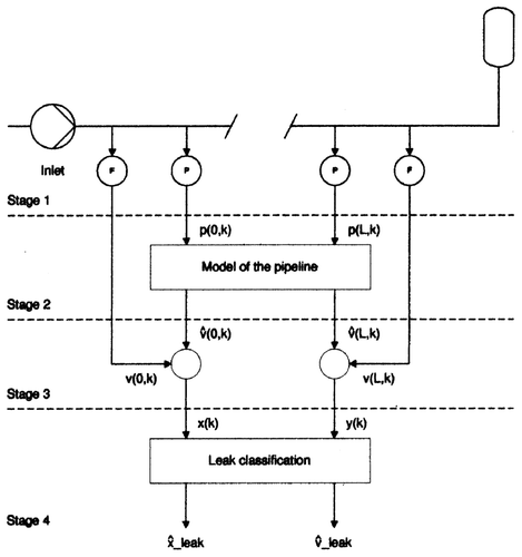
Observer-based leak monitoring requires a pipeline model in the form of a pipeline observer to compute the pipeline states assuming no leak. Further discussion will be focused on a discrete-time data-processing scheme. The difference between the measured and estimated flows at inlet and outlet, given by

where v(0, k) and [vcirc] (0, k) are the measured flow and the flow of the observer at the inlet of the pipeline, while v(L, k) and [vcirc] (L, k)) are the measured flow and the flow of the observer at the outlet of the pipeline, will be referred to as residuals. The leak flow and position can be estimated by

where L _p denotes the length of the pipeline 4. In order to eliminate flow measurement noise, a filter will be applied to the residuals leading to

with

In the above equations N is the depth of a first-in first-out buffer and should be chosen so as to be appropriate for the noise statistics. The leak position in (4) can be of course estimated only if the leak velocity [vcirc] _leak > 0. In practice a threshold is implemented, as shown later in Section 4. In figure 1, all basic parts of the described approach to the leak detection and classification can be seen.

Figure 1. Observer-based leak monitoring.

3 Models for the observer design

Observer-based leak detection and localization schemes require a pipeline model to compute the states of a pipeline without a leak 8,9. The basic mathematical model of a pipeline is a nonlinear distributed-parameters model. It describes the one-dimensional compressible fluid flow through the pipeline and is represented by a set of nonlinear partial differential equations 10. No general closed-form solution of these equations are known yet, and numerical approaches such as the method of characteristics must be used instead 11. If the pipeline is operating in the vicinity of a working point, a linear model can be exploited. The transfer function of such a model is obtained by the Laplace transformation of the linearized equations and corresponding initial and boundary conditions. The resulting transfer function is transcendent. Simple models of the pipeline in the form of a lumped-parameter system can be obtained by a Taylor series expansion of transcendental transfer functions. The resulting algorithms are less time consuming and hence better suited to critical real-time applications. With neural net models the grey-box approach is used. They are only an addendum to nonlinear distributed-parameter models; their structure is obtained from linear models, as are the initial values of the weights. After teaching, a nonlinear model is obtained. All four mathematical models of the pipeline will be given next. For simplicity reasons, outputs of the models (which are actually outputs of observers) will be denoted by p and v rather than by [pcirc] and [vcirc] respectively.

3.1 Nonlinear pipeline model with distributed parameters

The nonlinear pipeline model with distributed parameters is obtained by the application of the physical principles of mass conservation and Newton's second law. Applying these equation leads, under the assumptions that the fluid is compressible, viscous, isentropic, homogenous and one dimensional, to the following coupled nonlinear set of partial differential equations 5,11:

where p is the pressure, v the flow velocity, a the velocity of sound, the constant density of the homogenous fluid, α the pipeline inclination, λ the dimensionless friction coefficient and D the diameter of the pipeline. The continuity and momentum equations (6) and (7) form a pair of quasilinear hyperbolic partial differential equations in terms of two dependent variables, mass flow velocity v(x, t) and pressure p(x, t), and two independent variables, distance along the pipeline x and time t.

A general solution is not available; however, a transformation into the ordinary differential equation

along characteristic C + and

along C− with

is possible 12. These equations can be solved numerically using appropriate integration techniques; this method was realized in a special program PIPESIM. PIPESIM is written in C and consists of an application programming interface. User programs can use this application programming interface to solve (8) and (10) numerically.

3.2 Linear pipeline model with distributed parameters

The nonlinear equations (6) and (7) are linearized and written in a form using notation common in the analysis of electrical transmission lines. Also, the gravity effect can be included into the working point so that α = 0 is supposed. The corresponding system of linear partial differential equation is

where ( is the flow velocity at the working point) and are the inertance (inductivity), resistance and capacitance per unit length, respectively. Introducing the characteristic impedance Z_k  = [(Ls + R)/Cs]^1/2 and n = [(Ls + R)/Cs]^1/2, the linearized model of the pipeline can be written in one of the following four forms which differ from each other with respect to the model inputs (independent quantities) and outputs (dependent quantities): the hybrid representation with Inputs V ₀ and P_L, and outputs V_L and P ₀ given by

the hybrid representation with inputs V_L and P ₀, and outputs V ₀ and P_L given by

the impedance representation with inputs V ₀ and V_L, and outputs P ₀ and P_L given by

the admittance representation with inputs P ₀ and P_L, and outputs V ₀ and V_L given by

Linear models with distributed parameters were simulated by the convolution of the input time series and impulse responses of the corresponding transcendental transfer functions. The impulse responses were obtained by windowed and zero-padded inverse discrete Fourier transform of the frequency response.

3.3 Linear pipeline model with lumped parameters and low frequencies

Lumped parameters are described by rational transfer functions. One way to obtain the rational transfer functions from the transcendental functions given by (15) –  (18), is their extension into a Taylor series. There are seven different transcendental transfer functions in the four pipeline forms of Section 3.2: 1/cosh(nLp), 1/Z_K tanh (nLp), Z_K tanh(nL_p ), Z_K coth(nL_p ), Z_K sinh (nLp), 1/[Z_K coth(nLp)] and 1/[Z_K sinh (nLp)]. Each of the transcendental transfer functions of the impedance and admittance forms can be presented as a second-order transfer function. These models are only valid for low frequencies. Only admittance representations used in the observer-based leak monitoring will be given here and they are as follows.

1. Admittance representation: 1/Z_K coth (nLp). The input admittance at the downstream reservoirs (V ₀/P ₀) P_L  = 0. The negative output admittance at the upstream reservoirs (V_L /P_L ) P ₀ = 0. Also

   This transfer function describes the change in the flow velocity at one end of the pipeline if the pressure is changing at the same end while the pressure at the other end remains constant.

2. Admittance representation: 1/[Z_K sinh (nL_p )]. The negative reverse transadmittance at the upstream reservoir is −(V ₀/P_L )|P ₀ = 0. The transadmittance at the downstream reservoir is (V_L /P ₀)|P_L  = 0. Also

   This transfer function describes the change in the flow velocity at one end of the pipeline if the pressure is changing at the other end while the pressure at the same end remains constant.

Both transfer functions (19) and (20) have a static gain 1/(L_pR), which corresponds to the static change in the flow due to changing pressure.

3.4 Linear pipeline model with lumped parameters and high frequencies

The models derived in Sections 3.1 –  3.3 are valid predominantly in the low-frequency region. They do not include such phenomena as propagation of waves along the pipeline. Rather, oscillations due to the finite velocity of the waves is described as a second-order underdamped system. In this section a linear model will be derived which enables the preservation of the time delays inherently involved in distributed-parameter systems, such as pipelines. The flow at the outlet of the pipeline can be expressed from (18) as follows:

or, equivalently,

The same flow can be expressed also from (15) as

or, equivalently,

Adding (22) and (24) and dividing by 2, we obtain the equation which describes the dependencies of the outlet flow on the inlet flow and both (inlet and outlet) pressures:

In the same way the inlet flow can be rewritten from (18) as

or, equivalently,

It can also be written from (16) as

or, equivalently,

Adding (27) and (29) and dividing by 2, the equation which describes the dependences of the inlet flow on the outlet flow and both (inlet and outlet) pressures is obtained:

Thus (25) and (30) indicate that the flow on one side of the pipeline depends on the pressure on the same side (the corresponding transfer function is 1/Z_K ) and on the pressure and flow on the other side of the pipeline (the corresponding transfer functions are e^-nLp/Z_K and e^-nLp respectively).

3.5 Neural net model of the pipeline

The models derived in Sections 3.2 –  3.4 are linear models. The pipeline is, however, a nonlinear process. Neural nets are capable of modelling nonlinear phenomena; so it seems to be reasonable to apply them. However, neural nets are essentially lumped-parameter systems. Lumped-parameter models in Section 3.3 were obtained from distributed-parameter models in Section 3.2 by expanding the transcendental transfer function in Taylor series. Such models can easily be realized by a neural net; in fact there is only one linear neuron and some delays at the input and feedback. So one way to construct a neural net model is to extend a linear lumped-parameter model, that is a linear neuron, by one or several layers. A drawback of this model is that it does not involve the time delays that are inherently involved in a distributed-parameter model. Another way to design a neural net model of the pipeline is to use the models of Section 3.4. An attempt to approximate the transcendental transfer functions 1/Z_K  = (Cs)^1/2/(Ls + R)^1/2 and −exp((Ls + R)Cs)^1/2 L _P by rational functions was made in 13. Following the same paradigm a neural net could be designed but, since the square root has no Taylor series expansion around zero (in the above-mentioned paper the expansion was carried out by the Padé approximation and is not valid for s = 0), the long-term stability of such models is doubtful. The approach used in this paper is similar to the previously mentioned method; however, the neural net is used for correction only. The actual pipeline neural net model consists of two parts. The basic part is the nonlinear distributed-parameter model (the so-called PIPESIM model). Parallel to it there is a neural net correction model, with outputs [vtilde](0, k) and [vtilde](N, k), which are corrections of the inlet and outlet velocities respectively. The design of the neural net (and in particular the determination of the structure) is a matter of engineering feeling. Of great assistance in the present case are (25) and (30), which indicate that the flow at the inlet depends on the pressure at the inlet (transfer function 1/Z_K ), on the pressure at the outlet (transfer function e^-nLp/Z_K ) and on the flow at the outlet (transfer function e^{−mL _p} ). The sampling time of the neural net was chosen to be the same as for the PIPESIM program (0.1191 s). The number of segments in the PIPESIM model was N = 87. The transfer function e^-NLp involves a time delay (the time needed by waves to travel along the pipeline is N time steps). So N-step delayed signals of p(N) and v(N) are used as input to the neural net. An additional n input delays are used to enable the neural net to correct dynamic phenomena, which are not involved in the PIPESIM model. n was chosen to be 11, which is within 10 – 15% of the dominating time delay N. So the inlet and outlet velocity corrections can be written as

Two neural nets were used to realize (31) and (32). A three-layer (3 + 8 + 1 neuron) neural net, depicted in figure 2, has proven itself to be a suitable trade-off between complexity and time needed to be taught. The three-layer structure was chosen to mimic the PIPESIM structure: the equations for velocity and pressure and the nonlinear part; the quadratic dependence of the pressure drop on velocity. For simplicity reasons all signals were treated in the same way; so a tapped delay line with delays of 1 – 11 s was used at the input, which has made the neural net dynamic.

Figure 2. Neural net.

4 Application to a real pipeline

The models were tested using data obtained by a leak experiment on a real pipeline with the following data: pipeline length of L _p = 9854 m; diameter D = 0.2065 m, relative roughness k _c = 0.0602 mm; inclination α = −0.1948°. The fluid data were as follows: density ρ = 680 kg/m³; kinematic viscosity υ = 7.0 × 10⁻⁷ m²/s; source velocity α = 951 m/s. The stationary fluid velocity prior to the leak occurrence was 2.45 m/s. A 5% leak rate (0.1225 m/s corresponding to 14.77 m³/h) was generated at t = 437 s at 56.4% of the pipeline length where the outrunning fluid was filled into a tank lorry.

The parametrization of programs, a provision of the necessary data for the determination of the unmeasurable relative roughness of the pipeline and neural net training – verification data, was performed by another no-leak experiment with similar (2.46 m/s) stationary fluid velocity. In this experiment a shunt valve at the beginning of the pipeline was closed, leading to a quick drop in pressure and causing fluid transients. For the PIPESIM program, only the relative roughness was calculated from the stationary working point. For both linear models additionally the stationary working points (at the inlet and outlet respectively) of the above-mentioned experiment were used. The neural net was trained by the residuals (without leak) of the PIPESIM results. The TRAIN function of the MATLAB®'s Neural Net Toolbox 14 was applied using the Levenberg – Marquardt back propagation. The sizes of training and verification data were 12 000 and 9744 samples respectively and the number of epochs was set to 250.

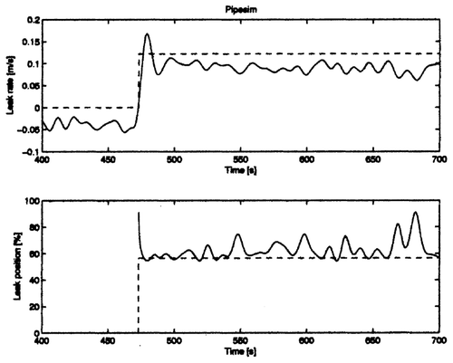
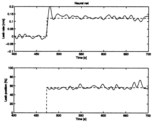
In figures 3, 4, 5 and 6 the filtered estimated leak rate and leak location are depicted for the PIPESIM model, the linear distributed-parameter model, the linear lumped-parameter model and the neural net model respectively. The leak position was evaluated only if a threshold of 2% was exceeded. Standard deviations (with respect to the real mean values) and deviations of the mean values of the rate and position errors for all models in percentages are depicted in table 1.

Figure 3. Estimated leak rate (upper) and estimated leak location (lower) for the PIPESIM model.

Figure 4. Estimated leak rate (upper) and estimated leak location (lower) for the linear distributed-parameter model.

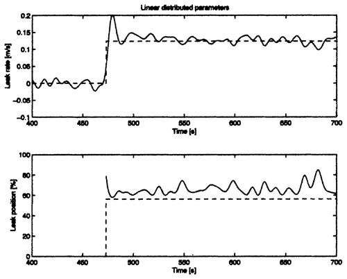
Figure 5. Estimated leak rate (upper) and estimated leak location (lower) for the linear lumped-parameter model.

Figure 6. Estimated leak rate (upper) and estimated leak location (lower) for the neural net model.

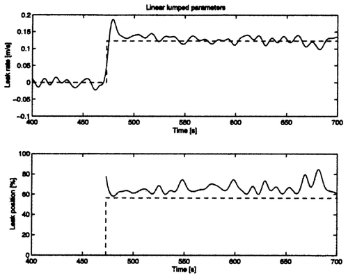
Table 1. Standard deviations and the deviations of the mean values of the rate and position errors for all models.

	Value (%) for the following models
	PIPESIM	Linear distributed	Linear lumped	Neural net
Standard deviation, rate	28.4249	8.7816	8.6543	9.3034
Standard deviation, position	9.4026	10.8520	10.8318	4.2284
Deviation of the mean value, rate	27.1487	3.0323	3.2328	3.8741
Deviation of the mean value, position	6.3811	9.6956	9.6815	0.5350

The PIPESIM program results were biased in the estimations of both the leak rate and the position. This was due to the bias in the fluid velocity sensors and due to the non-modelled dynamics. The bias of the sensors which were not eliminated with the PIPESIM program, and which contributed a major part to its bad rating, could be eliminated with some drawbacks, as explained in the conclusion. However, the neural net did exactly this in a more systematic way, which additionally incorporated the elimination of errors due to some non-modelled effects. All other models exhibited a small bias (approximately 3%) for the leak rate. This was probably due to the approximate evaluation of the real leak rate, which was obtained manually (it was not measured and registered); that is, the real leak rate was not 5% as considered in the evaluation, but 5.15%. Linear models used the working point of a similar experiment; so the offsets in leak rate (which are actually the differences of residuals) were eliminated. However, bias in the estimate of the leak position remained owing to non-modelled effects. Some of these effects were incorporated in the neural net model, which had the smallest bias of the estimated position.

5 Conclusion

Four models of the pipeline were used for leak detection and localization. The nonlinear distributed-parameter model was simulated using a special program PIPESIM. In its original form it served biased (in leak rate and position) results due to offsets in sensors and some non-modelled effects. Linear models eliminated the sensor offsets by definition; that is, offsets were eliminated by a longterm averaging technique. However, they provided useful results only for very small changes in the signals around a working point. Also they could not cope with comprehensive nonlinear effects of the pipeline; so the leak position estimate was biased. Best results were obtained with a neural net model as an addendum to the PIPESIM model. The neural net eliminated the sensor bias and incorporated some nonlinear effects which were not modelled by the PIPESIM program.

References

- Geiger , G. 1999 . “ Leak monitoring in pipelines—state of the art ” . In Seminar Fernleitungen der Landesanstalt für Arbeitschutz Kaiserau, , Germany 3 – 5 November 1999
- Geiger , G. , Werner , T. and Matko , D. 2003 . “ Leak detection and locating—a survey ” . In Proceedings of the 35th Annual Pipeline Simulation Interest Group Meeting Bern, , Switzerland 2003
- Isermann , R. 1994 . “ Integration of fault detection and diagnosis methods ” . In Proceedings of the IFAC Symposium on Fault Detection, Supervision and Safety for Technical Processes Espoo, , Finland 1994
- Geiger , G. 1998 . “ Application of a model-based method for leak detection and localization ” . In GMA-Kongress Meß- und Automatisierungstechnik, VDI Berichte 1397 18 – 19 June 1998
- Streeter , V. L. , Wylie , E. B. and Bedford , B. 1998 . Fluid Mechanics , 9th edition , New York : McGraw-Hill .
- Matko , G. , Geiger , G. and Gregoritza , W. 2000 . “ Verification of various pipeline models ” . In Proceedings of the 3rd International IMCAS Symposium on Mathematical Modelling Vienna, , Austria 2 – 4 February 2000
- Matko , D. , Geiger , G. and Gregoritza , W. 2000 . Pipeline simulation techniques . Mathematics and Computers in Simulation , 52 : 211 – 230 .
- Billmann , L. 1985 . Methoden zur Lecküberwachung und Regelung von Gasfernleitungen , Germany : Technische Hochschule Darmstadt . Thesis
- Siebert , H. 1981 . Untersuchung verschiedener Methoden zur Lecküberwachung bei Pipelines , Germany : Technische Hochschule Darmstadt . Thesis
- Streeter , V. L. and Wylie , E. B. 1978 . Fluid Transients , New York : McGraw-Hill .
- Anderson , J. D. 1996 . “ Basic philosophy of CFD ” . In Computational Fluid Dynamics , 2nd edition , Edited by: Wendt , J. F. Berlin : Springer .
- Streeter , V. L. and Wylie , E. B. 1993 . Fluid Transients in Systems , London : Prentice-Hall .
- Matko , D. and Geiger , G. 2002 . Models of pipelines in transient mode . Mathematical and Computer Modelling of Dynamical Systems , 8 : 117 – 136 .
- The MathWorks, Inc. Neural Network Toolbox License number 190357