Application of ellipsoidal estimation to satellite control design

Abstract

The equations of motion of a small satellite moving along a prescribed trajectory under disturbances are analysed. Problems of this kind have been extensively investigated. The corresponding equations for relative motion errors, caused by the uncertainties in initial conditions and control implementation imperfections, are linearized. The linear equations are reformulated and the evolution equations for optimal ellipsoidal estimates of these errors are derived. It is shown that ellipsoidal bounding of reachable sets is an efficient approach to model uncertain linear dynamical systems. The procedure constructed in this paper allows one to take into account discrete observations and to design control aimed at compensating the disturbances between measurements. These measurements are assumed to be performed with small errors. A numerical example is given which illustrates that the presented control design algorithm is quite efficient and allows one to keep the error between the real and desired motion close to zero.

Keywords:

• Uncertain dynamical systems
• satellite control
• ellipsoidal estimation
• reachable sets

1. Introduction

Multiple spacecraft formation flying is emerging as an enabling technology for a number of missions of NASA and other space agencies. Various aspects of this problem are addressed, e.g. in [1 –  4]. In this paper a guaranteed ellipsoidal estimation approach is applied to the problem of follower (slave) satellite motion with respect to another leader (master) satellite. It is assumed that the trajectories of both the leader and follower are close to quasi-circular elliptic orbits. The problem of designing a control algorithm, as presented below, is examined for the follower satellite only.

Consider the motion of both leader and follower satellites along the same circular orbit at an altitude of 630 km above the Earth's surface with a speed of 7500 m/s. Let us compare two follower satellite control strategies: applying a small control (of fixed absolute value) transversally or tangentially with respect to the trajectory. Figures 1 and 2 show that the small transversal change of velocity leads to a more significant orbit modification, while the tangential one just causes oscillations in the vicinity of the original motion. Hence we will focus on ‘transversal’ control.

Figure 1. Motion for the case of a tangential change of velocity (a) with respect to the Earth for the 1 m/s change in the same direction as the initial satellite motion, (b) the same change in velocity, with motion with respect to the master satellite, (c) relative motion for 1 m/s change in velocity in the direction opposite to the master satellite motion.

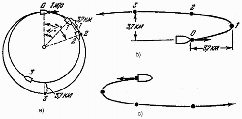
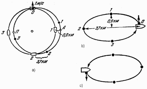
Figure 2. Motion for the case of a transversal change of velocity (a) with respect to the Earth for the 1 m/s change in the upward direction, (b) the same change in velocity, with motion with respect to the master satellite, (c) relative motion for the 1 m/s change in the downward direction.

Figures 1 and 2, as well as the results given in [5] and [6], suggest that the transversal maneuver is more fuel efficient. Hence in section 4 we consider the control to be transversal. It will be seen later that the tangential control could also be easily incorporated in the framework of the results presented below.

2. Initial equations

In this section the motion of the follower satellite is examined (below the term ‘follower’ is omitted). The motion of a satellite, subject to the Earth's gravitational field and to control forces, is considered in an inertial Cartesian coordinate system with its origin at the Earth's centre. The units for the variables have been chosen in such a way that the mass of the follower satellite takes a unit value. Then its trajectory is obtained as a solution of the following system of differential equations:

In the absence of control

With assumptions (3), equations (1) and (2) can be integrated. Define the initial conditions for (2) in the form

where υ _i are specific orbital parameters. The solution of (1) with initial conditions (4) can be presented in the form

Relations (5) allow the use of υ₁, … υ₆ as new (osculating) coordinates introduced by these formulas for the case in which (3) does not hold. Plugging in the coordinates (5) into the equations (1) we obtain

Note that (5) implies that the functions F_i are solutions of (1) with zero u_i , so (∂F_i /∂t) = X_i , thus,

In the next section the osculating variables, which are convenient for further use, will be introduced and the equations in these coordinates will be derived.

3. Equations in osculating variables

The solution of (1) with assumptions (3) comprises an elliptic orbit. Introduce the osculating variables

for this solution. Here A is the largest semi-axis of the elliptic orbit, ε is its eccentricity, i is satellite orbit inclination, and Ω is the longitude of the ascending node. The angles φ_π (between the largest semi-axis and the node line) and v (the true anomaly) together with the other variables

and the three-dimensional vector of acceleration {a_R ,a _Φ,a_N } are presented in figure 3.

Figure 3. Variables for (6) .

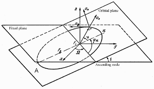
Figure 4. s ₁ = 01.

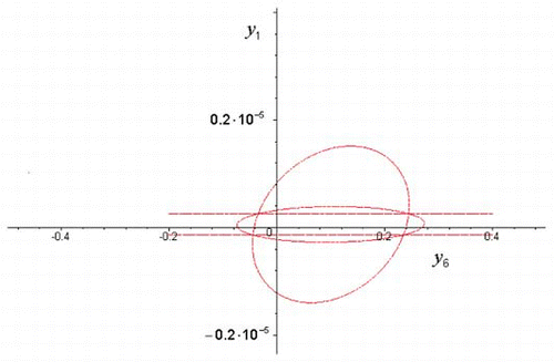
Figure 5. s ₂ = 0.2.

Then the equations (6) take the form:

The functions introduced in (7) are given below

The functions in (8) define the right-hand sides for the system of equations in (7) in terms of

which becomes singular for ϵ→0. To avoid this we use another set of variables υ = {p,L,K,Ω,i,s}, where

Here in (9) p is a focal parameter, L and K are the Laplace vector components, and s is the latitude. As for the variables in

as above, Ω is the longitude of the ascending node and i is the inclination of the satellite orbit. The variables in

could also be expressed via variables in υ:

Thus, for these variables the following equations can be derived from (7) and (10):

Here the functions G_A, G _ε, G _φ, G _ν , G_i, G _Ω, as defined by (7) and (8), are calculated using the variables in

expressed via our new variables in υ through the relations (10), providing functions G_A (υ), G_ε (υ), G_φ (υ), G_γ (υ), G _Ω(υ), G_i (υ). The equations obtained in this way provide a system of ordinary differential equations for υ. In the next section additional assumptions allow us to simplify this system and to linearize it.

4. Additional assumptions

The following assumptions are used to simplify equations (11).

(1) The motion is considered in the vicinity of the quasi-circular orbit (with eccentricity

).

(2) Acceleration has a constant absolute value (during a given time interval) and is collinear with the velocity.

This means that in (7) a_R ≡a_N ≡0, a _Φ = u≡const. This control is designed to correct the orbit and make the motion closer to the prescribed one at some further time instant (e.g. at the right end of the given time interval). Then equations (11) transform into the following system:

Introduce the latitude s of the satellite as a new independent variable. Denote by z the vector z = z(s) = {p,L,K,Ω,i,t}. Then the initial conditions in (12) can be rewritten as z(s ₀) = z ⁰ = {p ₀,L ₀,K ₀,Ω₀,i ₀,t ₀}. Define the error vector

Now consider the linearized equations. We assume that both acceleration u and eccentricity ϵ are small (

,

). Linearization means that for all the relations of y, considered below and implied by (7) and (12) and (13), we neglect all terms with an order higher than 1 (e.g. u ², ε², and εu).

To estimate the set of possible satellite deviations from a given elliptic orbit, the outer ellipsoidal estimations of reachable sets [1, 2, 6 –  9] are constructed.

5. Linearization and ellipsoidal estimates

On each interval of movement the small imperfections in control actuation and uncertainty in initial conditions must be taken into account. These control disturbances are presented by the vector w as defined below. For the variable y the linearization of equations (13) (based on relations (7) –  (12)) results in the following formulas:

where

Here δu is the error in the absolute value of u, δα is the angle between the projection of the (perturbed) acceleration vector onto the plane containing the prescribed orbit and perpendicular to the radius vector, and δβ is the angle between the (perturbed) acceleration vector and the plane containing the prescribed orbit. Denote by E(a,Q) an n-dimensional ellipsoid

where a∈R ⁿ is its centre, Q is a positive definite n × n matrix, and (·,·)denotes the scalar product of vectors. For the initial value of s ₀, the new independent variable s, the following assumptions are made:

Introduce for s = s_k , k = 1,…, n, the values

, i.e. measurements of the first component of the vector y:

. Define

, Here the absolute values of measurement errors e_k are bounded by the inequalities

. The values of Q ₀, R(s) (for all s), and

are assumed to be known. The observations, with these error bounds imposed, define the sets M_k compatible with the results of observations:

Measurement of the first component is considered for the sake of simplicity; measurements of various components could be processed analogously. For each interval [s_k ,s_{k  + 1}], k = 0, …, n we construct the outer ellipsoidal estimate E(a(s),Q(s)) containing all the solutions of (14) with constraint (16). We also take into account observation results (17) and arrive at the following recurrent procedure. For the evolution of parameters a, Q (with the volume of the ellipsoid taken as the optimality criterion) on the interval [s_k ,s_{k  + 1}], k = 0, …, n the following equations hold (see, e.g. [7 –  11]):

u = u_k to be chosen later, and the initial conditions for (18), (19) are

Here

. For k > 0 we obtain values of

and

recursively. Firstly we solve equations (18) and (19) on the interval [s_{k  – 1}, s_k ] with initial conditions

,

and obtain the values

for these solutions at the right end of the interval.

Secondly, we define the values of

and

from the inclusion

where

is the minimum volume ellipsoid containing this set.

We choose a small constant control u = u_k ,

in (18) and (19) for s∈[s_k ,s_{k +1}] to minimize the length of the vector a_{k +1}, which defines the centre of the ellipsoidal estimate E_{k +1} at the right end of the interval, according to equations (18) and (19) and initial conditions (20). Denote by

the fundamental matrix of the system (18). For Φ _u (s) the following equation holds

with initial conditions

where I is the identity matrix. Introduce the notation

. Relations (21) and (22) imply the equation

with initial conditions

Solutions of equations (21) and (23) with initial conditions (22) and (24) provide the values of the matrix functions

,

for s∈[s_k ,s_{k  + 1}]. Note that on the interval [s_k ,s_{k  + 1}] the solution of equation (18) with initial condition (20), due to relations (21) and (22), can be written in the form

Thus, minimizing the length of the vector a(s_{k +1}) yields

is to be minimized.

Formula (26) implies the necessary condition

Finally, the values u_k  = ± U should be tested together with all roots of (27) inside the interval |u_k | ⩽ U. Then u _k minimizing the value

should be chosen.

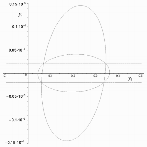
6. Example

Consider the system (12) with L ₀ = 0.001, p(0) = 1, K ₀ = Ω₀ = i ₀ = s ₀ = 0. We construct the equations (18) and (19) for ellipsoidal estimates of y. In the relations (16) we assume that

is the only non-zero element of the matrix Q ₀ and is equal to

and R≡0. Then, all the deviations on position of y are implied by the initial conditions (28) and the measurement error is

. Figures 4 – 5 contain simulation results for s ₁ = 0.1 and s ₂ = 0.2.

The projections of the ellipsoids onto the plane {y ₁,y ₆} are presented. The initial value of y was assumed to be

and the errors of measurements

simulated for s = s_k, k = 1,2, where

. Note that y ₆ = t and only the value of y ₁ is to be minimized. The value of u_k was chosen according to the procedure given in the previous section, with U = 10^– 7. The chosen control, for given instances s_k in the numerical simulations, allows one to govern the first coordinate y ₁ of the centre of the ellipsoidal estimates closer to zero than the measurement error

.

7. Conclusions

The presented ellipsoidal state estimation procedure provides control design under given bounds on uncertainties in the presence of noisy discrete observations. The example shows that this control design algorithm is quite efficient and allows one to keep the error between the real and the desired motion close to zero.

Acknowledgements

This work was partially supported by the Russian Foundation of Basic Research (Grant 02-01-00201) and by the Grant of the President of the RF for leading scientific schools No. 1627.2003.1 and by the Royal Society, UK.

References

- McInnes , CR . 1995 . Autonomous ring formation for a planar constellation of satellites . Journal of Guidance, Control, and Dynamics , 18 : 1215 – 1217 .
- Wang , PKC and Hadaegh , FY . 1996 . Coordination and control of multiple microspacecraft moving in formation . Journal of Astronautical Sciences , 44 : 315 – 355 .
- Ukybyshev , Y . 1998 . Long-term formation keeping of satellite constellation using linear-quadratic controller . Journal of Guidance, Control, and Dynamics , 21 : 109 – 115 .
- Beard , RW , McLain , TW and Hadaegh , FY . 2000 . Fuel optimization for constrained rotation of spacecraft formations . AIAA Journal of Guidance, Control, and Dynamics , 23 : 339 – 346 .
- Okhotsimsky , DE . 1964 . Investigation of motion in the central field for a satellite subjected to a constant transversal acceleration . Space Research , 2 ( No. 6 )
- Grodzovsky GL Ivanov JN Tokarev VV 1975 Mechanics of the Space Flight Moscow Nauka (in Russian)
- Chernousko FL 1994 State Estimation for Dynamic Systems Boca Raton CRC Press
- Milanese M Norton J Piet-Lahanier H Walter E (Eds) 1996 Bounding Approaches to System Identification New York Plenum Press
- Kurzhanski AB Valyi I 1997 Ellipsoidal Calculus for Estimation and Control Boston Birkhäuser
- Chernousko FL 1999 What is ellipsoidal modelling and how to use it for control and state estimation? In: I. Elishakoff (Ed.) Whys and Hows in Uncertainty Modelling Vienna Springer pp. 127 – 188
- Chernousko FL 2002 On optimal ellipsoidal estimation for dynamical systems subjected to uncertain perturbations Cybernetics and Systems Analysis No. 2 pp. 85 – 95