Optimal control of biological SBRs for the treatment of dairy and toxic wastewaters

Abstract

This paper presents two optimal control strategies developed for the control of two biological sequencing batch reactors (SBR), the first one performing both organic carbon and nitrogen removal from dairy wastewaters, while the second one treats toxic wastewaters. The proposed control laws are based on models that have been validated with real data acquired on two real biological SBR pilot plants. These models are presented in D. Mazouni et al., 16th IFAC World Congress, Prague, 5–8 July 2005. The validation results of these control strategies are presented and discussed.

Keywords:

• sequencing batch reactors
• optimal time control
• optimization

1. Introduction

The objectives of the control module that was developed within the EOLI integrated system were twofold: first, developing an algorithm for the optimal control of the SBR in the presence of an inhibiting reaction scheme, and second, developing a time optimal control strategy for the control of aerobic SBRs with carbon and nitrogen removal capacities.

These model-based control laws are directly derived from the models proposed in 1. They also take into account the information about direct measurement (via hardware sensors) presented in 2 and about the indirect measurement (via software sensors) proposed in 3. Because of the type of operation (which is a batch), optimal control is the core of the control design to optimize the following: (i) the feeding strategy by distributing the feed with time to avoid accumulation of toxics and/or inhibitory substances in the cases of toxic effluents; and (ii) the aerobic and anoxic phase time durations to minimize the total reaction time in the case of carbon and nitrogen removal.

2 Carbon and nitrogen removal from dairy wastewaters

2.1 The process

The objective of the control is to compute the switching sequence (aerobic/anoxic) and the corresponding switching instants such that any initial point in the attainable set reaches the target set (defined as the set of concentrations such that S ₁ < S _1N , S ₂ < S _2N and S ₃ < S _3N ), where S ₁ is the soluble COD, S ₂ is the ammonium nitrogen concentration, S ₃ the ammonium nitrite + nitrate concentration, and S _1N , S _2N and S _3N are the normative rejection norms.

The minimal time optimal control is based on a simple model directly derived from those presented in [1]. This model is briefly reported hereafter. A schematic view of the process available at the LBE, Narbonne, France, is given in Figure 1.

Figure 1. Schematic view of the process.

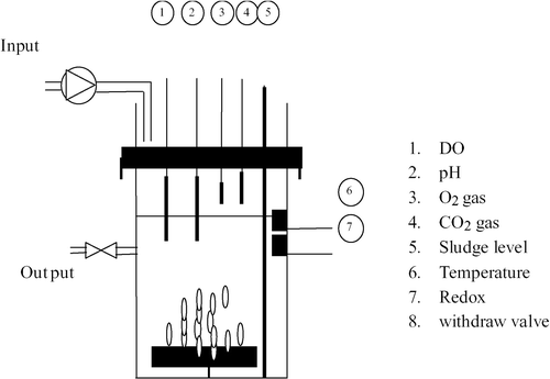
The tank of the reactor has a cylindrical form. Its dimensions are 50 cm ø and 130 cm height with a total volume of 255 l. It is equipped with a variable flow rate pump to fill the reactor and a controlled valve to withdraw the effluent and the sludge in excess. Air is used for aeration and mixing. Its flow is controlled by a flow meter.

The reactor is operated at an ambient lab temperature of 20°C. Each cycle duration is 24 h. More specifically, the reaction phases are divided into two periods. In each one, half of the total influent daily volume is added (25 l). A schematic view of the operating mode is shown in Figure 2.

Figure 2. Schematic view of the classical alternating aerated conditions.

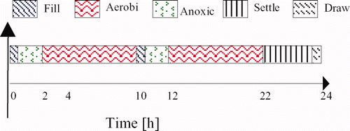
Because both the carbon and nitrogen are treated, two specific phases are needed: aerobic (presence of oxygen) and anoxic (no oxygen but nitrite and nitrate). During the anoxic phase, the nitrite and nitrate from the last cycle are transformed into gaseous nitrogen. This step is realized by heterotrophic bacteria, which also need soluble organic carbon to grow; cf. 4 or 5. When all the nitrite–nitrate has been removed, one can switch to aerobic mode where the ammonium nitrogen will be transformed into nitrite and nitrate while the remaining soluble carbon will be removed.

From now, we only concentrate on what happens during the aerobic phase and the following notations are used: X ₁, heterotrophic microorganisms (mg/l); X ₂, autotrophic microorganisms (mg/l); S ₁, organic carbon (mg COD/l); S ₂, ammonium nitrogen (mg N-NH₄/l); S ₃, nitrates/nitrites nitrogen (mg N-NO₃/l + mg N-NO₂/l); S ₄, dissolved oxygen (mg O₂/l).

2.2 Modelling

The reaction scheme of the aerobic phase is as follows:

This synthetic scheme means that S ₁ and S ₂ are degraded by X ₁ and X ₂, respectively, with the rates ϕ₁ and ϕ₂ in the presence of S ₄. In other words, the pollutant S ₁ serves as a basis for the growth of X ₁, while S ₂ is transformed into S ₃ by X ₂.

Considering the above reaction scheme, we can apply the mass balance principle to determine the state space model of the aerobic phase 6:

with

As can be seen, the specific growth rates in the aerobic phase, μ₁ and μ₂, are proportional to the dissolved oxygen concentration, S ₄, in the reactor instead of the classical expression proposed in 7. It is essentially because the available experiments were realized with a nonlimiting oxygen concentration, S* being the average of residual COD in the reactor 1. Furthermore, if it is assumed that the oxygen is not limiting, then the differential equation describing the time variation of the oxygen can be omitted. Using the mass balance conservation principle in a batch reactor, it is then possible to show that the above system can be reduced to the following third-order dynamical system:

which can itself be put under the following compact form:

where Z ^T  = [S ₁, S ₂, S ₃] and where all functions and parameters depend on the original model (2) to (8).

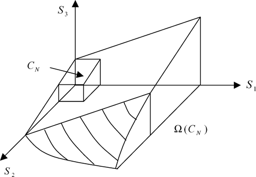
The first task is to characterize the attainable set, that is characterizing the set of initial conditions for which there exists a control sequence, thus defining a trajectory, that drives the initial point towards the final target set defined as {S ₁ < S _1N , S ₂ < S _2N , S ₃ < S _3N –αS_2N}. The details of this study are reported in 8 and the attainable set is represented graphically in Figure 3.

Figure 3. The attainable set.

2.3 Control design

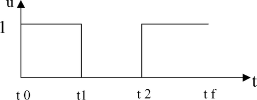
From now onwards, it is supposed that X ₁(0) ≠ 0 and X ₂(0) ≠ 0. Once it has been verified that there exists a trajectory allowing us to drive the state toward the final set, it is of interest to compute the control actions (switching instants between aerobic and anoxic phases) in order to do so. Within the set of all possible switching policy and to keep the problem tractable (in practice, it is not possible to switch too often), it was decided to limit the computation to the search for control sequences comprising only two switches at most. In other words, the class of optimal control sequence to be applied can be schematically represented in Figure 4.

Figure 4. The class of admitted optimal control sequence to be applied.

Indeed, it should be noted here that any initial condition within the attainable set can be driven toward the final set in applying the specific sequence {aerobic, anoxic, aerobic}; cf. 9.

The problem to be solved can now be reformulated as the search for the two switching instants t ₁ and t ₂ such that any initial condition in the attainable set is driven toward the final set in a minimum time:

Unless the optimal solution be u = 0 (it means that there is almost no ammonium nitrogen (S ₂) in the effluent, that is when S ₂(t ₀) < S _2N ), two distinct cases can arise: either the optimal trajectory first reaches the plane defined by S ₁ = S _1N or the one defined by S ₂ = S _2N . Since both concentrations S ₁ and S ₂ must verify S ₁(t _f ) < S _1N and S ₂(t _f ) < S _2N , the problem can be rewritten as the search for t ₁ and t ₂ such that:

be minimal.

To solve the general case (find the switching instants for t ₁ and t ₂ of the control sequence aerobic/anoxic/aerobic), the maximum principle is first used. Using this principle, it is possible to show that there exists a switching plane that defines the commutation instant t ₂. To compute t ₁, an optimization problem is solved numerically: it corresponds to the search for t ₁ that minimizes the anoxic phase time period. During anoxic phases, u = 0. Thus, S ₂ is constant while S ₁(t) and S ₃(t) are linearly related referring to the relationships obtained from the first integral . To parameterize the anoxic phase time period, we introduce the following variable: such that S ₁ = S ₁(t ₁)−θ and S ₃ = S ₃(t ₁)−βθ. Let δ be the variation of S ₁ in the anoxic phase (it is proportional to the variation of S ₃ over the same period). It is given by . The anoxic phase time period is then given by:

where is the solution of the dynamical system (10) for u = 1 at t = t ₁.

2.4 Results and discussion

The biological interpretation of the optimal solution is as follows. The nitrogen removal kinetics is very slow compared to the carbon removal. Thus, the required aerobic time corresponds essentially to the nitrogen removal. Since nitrogen is not eliminated in the anoxic phase, the aerobic phase duration cannot be minimized. We can only reduce the total cycle time by reducing the anoxic phase time.

In standard cases, the anoxic phase takes place at the beginning of the cycle. The anoxic reaction rate depends on the two substrate concentrations S ₁ and S ₃. At the beginning, the maximum of carbon is available. In most cases (depending on the initial conditions), the optimal control strategy consists in starting with an aerobic phase to maximize the anoxic reaction rate. During the first aerobic phase, S ₃ increases and S ₁ decreases. The anoxic phase is applied when the maximal possible rate of the anoxic reaction is reached, so that the total time of this phase is reduced. Of course if the maximum anoxic rate is given at the initial time, the batch starts with the anoxic phase as in the classical approach the total time cannot be further reduced.

Hereafter, we present a comparison between the application of a classical control sequence based on a constant time period approach (anoxic/aerobic) and the above presented optimal control approach. Initial conditions are about S ₁(0) = 700 mg/l, S ₂(0) = 50 mg/l, and S ₃(0) = 30 mg/l. The switching instants were computed offline using the influent characterization and the initial biomass concentrations ( Table 1).

Simulation results are presented hereafter ( Figure 5).

Figure 5. Phases duration comparison with real data.

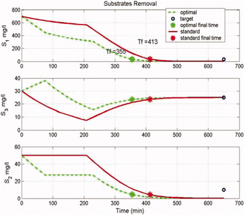
Table 1. Phases duration comparison with real data.

	Anoxic time (min)	Aerobic time (min)	Total
Classical cycles	32	390	422
	35	410	435
	30	400	430
Optimal control approach	28	10 + 380	418
	25	10 + 360	395
	26	10 + 380	416
	22	10 + 400	432
	24	10 + 390	414

The optimal approach was applied with several replicates. Globally, the average of the anoxic phase duration in the standard case was 32 ± 3 min and the aerobic phase was 410 ± 15 min. With the optimal approach, the average of the anoxic phase time was around 25 ± 5 min and the aerobic phase was 390 ± 20 min. The time reduction for the anoxic phase is around 13% while the total reaction time was reduced by only 4%. This happens because the long aerobic phase depends essentially on the nitrogen removal, which is not eliminated in the anoxic phase. The anoxic reaction time is reduced by increasing the anoxic reaction rate.

3 Treatment of toxic wastewaters

3.1 The process

For the toxic wastewater treatment, the SBR sequence is similar to the one depicted in Figure 2 (in Section 2), except that there exists no anoxic phase. This means for this case there is only one single aerobic phase. The classical batch operation mode of the SBR feeds the influent all at once at the beginning of the cycle. This causes an inhibition of the biomass, due to the excessive toxic concentration fed, that renders the reaction inefficient. The time optimal control (TOC) objective is chosen as to minimize such a reaction time by controlling the feeding rate using a fed-batch mode. The problem for implementing the TOC is the lack of online measurements for the substrate and biomass concentrations both in the SBR tank and/or in the influent flow. Because of such a limitation, even having a good mathematical model for the process is not enough to optimally control it.

3.2 Modelling

The reaction scheme of the reaction phase is

which, assuming that the dissolved oxygen is not limiting, that the biomass decay is negligible and that no biomass nor oxygen are fed via the influent, leads to the mass balance based model:

where 0 < Q < Q _max is the inflow volumetric flow (l/h); V ₀ ≤ V ≤ V _f , volume level of the liquid in the tank (l); S, toxic concentration in the tank (mg COD/l); S _in, toxic concentration in the influent (mg COD/l); S ₄, dissolved oxygen concentration (mg O₂/l); S _4,sat, saturation value of the dissolved oxygen concentration in the liquid medium (mg O₂/l); k _L a, oxygen mass transfer coefficient (h⁻¹); b > 0, endogenous respiration coefficient (h⁻¹); and μ, specific biomass growth rate (h⁻¹).

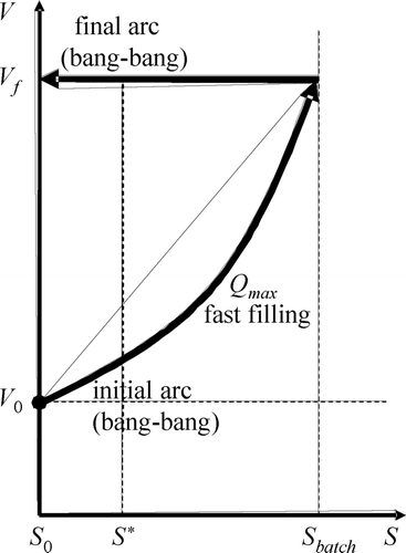
The main characteristic of the model structure is the inhibitory effect that the toxic concentration does have on the biomass behaviour, represented by μ in Figure 6. Let us call S* the toxic concentration at which it reaches its maximum value (μ*). Such a point is where inhibition just begins. S _batch represents the toxic substrate concentration value that is reached inside the SBR when the filling process finishes using the typical batch mode. Such a fast filling process is represented by the first arc of the substrate-volume (SV) trajectory projected in Figure 7. This action takes the volume quickly from its initial value (V ₀) to its final one (V _f ), thus increasing the concentration inside the tank from its initial value (S ₀) to its maximum value during the reaction (S _batch). Relating Figure 7 to Figure 6, it is easy to see that the batch reaction gets inhibited soon after the beginning and will stay so until the substrate is degraded down to the S* value, which usually is accomplished only at the final stage of the reaction. As a consequence, a typical batch reaction spends most of its time inhibited.

Figure 6. Inhibitory specific biomass growth rate.

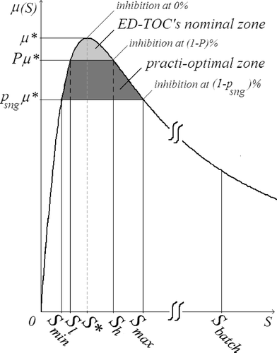
Figure 7. Typical batch SV-trajectory.

3.3 The control design

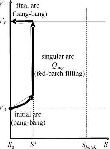
Results useful to optimize a batch process as the one producing the trajectory in Figure 7 are already available in 10-12. The exact minimum time trajectory is shown in Figure 8. It does have three arcs. The initial and final arcs are of the bang type, meaning there are either maximum or zero input flow applied at any given moment. The intermediate arc, however, should live in the singular surface (S = S*), and, thus, the inflow should be controlled exactly as calculated by 10:

The problem for calculating such a singular flow is that the values of S, S _in and X are not available online.

Figure 8. Nominal (ideal) TOC SV-trajectory.

Assumption 1: S _in ≫ S* > S ₀

Assumption 2: Q _max > Q _sng

Assumptions 1 and 2 are natural conditions for the problem. The first one guarantees that the initial bang arc may be one of the ‘fill’ type (i.e. Q = Q _max) while the second one guarantees that dS/dt > 0 during such a fill arc if it started to the left of the singular surface. Note that, on the other hand, a bang ‘react’ arc (i.e. Q = 0) will always comply that dS/dt ≤ 0. Note that fill arcs generate trajectories that grow both in V and in S (e.g. the initial arc in Figure 8) while react arcs generate horizontal trajectories of constant V and decreasing S (e.g. the final arc).

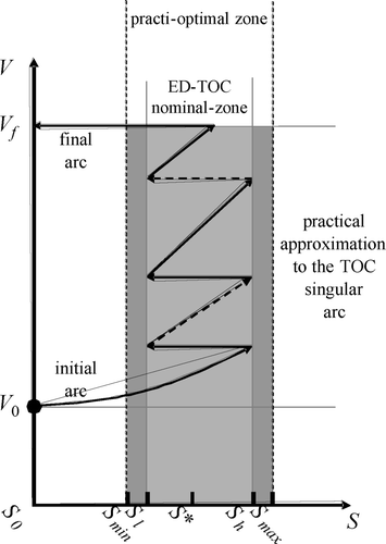
Let us define as practically optimal (practi-optimal) a controller whose trajectory performs the initial and final arcs of the TOC exactly but only approximates the singular one. Figure 9 shows a way to describe the acceptable approximations, the ones which approximate (arbitrarily well) the singular arc inside a given tube defined by S _min < S < S _max such that, inside such a tube, μ > p _sng μ*, as depicted in Figure 6.

Figure 9. Practical TOC SV-trajectory.

Model based observers to estimate S using the volume level and the dissolved oxygen (V, S ₄) have been used in a feedback control to implement a practi-optimal solution in a lab-scale SBR 13. However, it required the (normally unavailable) values of X and S _in to operate properly, and so its practical use in real wastewater treatment plants was not feasible. Next, a practical approximation to the TOC that uses also V and S ₄ but that does not require the unavailable measurements will be presented.

3.4 Event driven TOC

The idea to implement the event driven TOC (ED-TOC) is to perform the approximation of the singular arc by iteratively switching the influent flow (Q), on–off, in such a way as to generate a bang-bang trajectory shaped like a zigzag composed of fill (on) and react (off) arcs ( Figure 10). Note that each pair of consecutive fill-react arcs resembles a mini-batch. The resulting trajectory is practi-optimal if all mini-batch arcs reside inside the allowed practi-optimal zone. To guarantee that such is the case, even if there are bounded perturbations in the measured variables, the ED-TOC targets an inner “nominal-zone” defined by a tuning parameter p _sng < P < 1 ( Figure 6), which allows to choose the nominal switching surfaces S = S _l and S = S _h . Note that by choosing P ( Figure 6) arbitrarily close to one renders the practical approximation in Figure 10 arbitrarily close to the exact optimal one in Figure 8.

Figure 10. ED-TOC SV-trajectory.

If S was available and S _l , S _h were well known, then detecting the events related to the crossing of the switching surfaces ( Figure 10), by using a set of comparators, would be straightforwardly easy. However, that is not the case. Instead, the idea behind the ED-TOC is to use the knowledge about the model structure to perform an estimation of such events needed to drive the controller. Next, a simplified three steps explanation into the workings of the ED-TOC follows: (1) a way to compute the oxygen mass uptake rate (OMUR) using only the available data will be derived; (2) the use of a hypothetical variable (denoted γ) to detect the events needed to drive the ED-TOC will be explained; and (3) a justification for using the OMUR instead of γ for performing a practi-optimal ED-TOC will be given.

(1) The OMUR may be defined as the volume multiplied by the oxygen uptake rate (OUR) and then (14) maybe rearranged to compute it as

where B := XV is the total biomass, k ₄μB is related to the exogenous respiration, which in turn is directly proportional to the substrate reaction rate, and bB is related to the endogenous respiration. Note that the right-hand side of this equation is computable online as every term there is known or measurable.

(2) Let us assume that the function

is available online, where B ₀ := X ₀ V ₀ is a positive constant representing the initial total biomass. Then, it is possible to relate the switching surfaces directly to γ by defining γ* = k ₄μ*B ₀ and γ = Pγ* as the surface where either S = S _l or S = S _h . To differentiate which one of such events is the one really happening it suffices to know the sign of the derivative of γ and the state of Q. If the arc being produced is of the react type, then a decreasing γ means that the trajectory is on the left side of the singular surface, and, thus, the switching occurs for S = S _l . On the other hand, if the arc is of the fill type, then the same decreasing behaviour of γ means that the trajectory is on the right side of the singular surface, and, hence, the switching occurs for S = S _h .

Using such information it is easy to implement the nominal ED-TOC, exactly as in Figure 10, as follows: first (using assumption 1), apply Q = Q _max to produce a fill type arc. Once γ reaches a maximum and begins to decrease, the singular surface was crossed from left to right. Such a maximum is γ*. Keep filling until γ = Pγ*. At this point, the event of crossing S = S _h is detected and the filling is stopped. Then, a react type of arc begins and the behaviour of γ repeats itself, i.e. it will increase again until a maximum (γ*). At that point, the controller knows the singular surface is being crossed, this time from right to left. Then, when γ decreases down to Pγ*, the event of crossing the switching surface S = S _l is detected and a new fill arc begins. Such a fill-react-fill cycle is repeated until the tank gets full.

(3) The type of processes under study is of the substrate degrading type and not of the biomass producing ones. This means that the total biomass increase (ΔB = B _f  − B ₀) is negligible (ΔB ≪ B ₀) during a single batch. Additionally, in a properly designed toxic wastewater treatment system, the endogenous respiration is much less than the exogenous one when the process is taken near to the singular surface (k ₄μ*B ≫ bB). Using these conditions in the left-hand side of (16), it is easy to see that, inside the practi-optimal zone ( Figure 10), the error in detecting the events of the crossing of the switching surfaces is low if the OMUR is used instead of the ideal γ in (17), for implementing the ED-TOC, because

A complete explanation of the ED-TOC and a robustness analysis, including the effects of the biomass growth and the endogenous respiration, when they are not negligible, is given in 14.

3.5 Experimental results

The ED-TOC, using the computation of the right-hand side of the OMUR in (16) directly instead of the ideal γ in (17), was applied to the treatment of a synthetic wastewater containing 4-clorophenol (4CP) as a toxic model compound. A 7-l lab-scale SBR was used with an exchange volume of 53%. The influent toxic concentration defined as the standard condition was 3500 mg 4CP/l. Multiple ED-TOC fed-batch experiments were performed for both the standard condition and for load shocks. The shock load consisted of increasing the influent toxic concentration up to 20 times the standard one, as a perturbation of the standard operating condition. A comparative analysis was made versus the pure batch operation mode. It must be noted that the pure batch operation mode is not able to withstand unknown perturbations higher than three times the standard condition, because the inhibition caused to the biomass is so high that it becomes irreversible and the SBR is disabled. Then, to be able to compare data, it was assumed that the perturbation was known (as if the influent concentration S _in was measurable) and a predilution of the influent to the standard condition was allowed for the pure batch case (not for the ED-TOC case). This means that multiple pure batches were required to treat the same amount of influent that the ED-TOC was able to treat in a single fed-batch during the shock load perturbations.

The improvements, over the pure batch mode, for using the ED-TOC, as reported in 15 may be summarized as follows: (1) a reduction in total batch time that allowed increasing the daily applicable load in a range from 63% up to 90%, both in standard and in shock load conditions; and (2) savings in energy between 25% and 39% represented in less aeration and stirring time required during the reaction phase.

4 Conclusions

In this paper, two optimal control strategies for two types of biological processes performed in sequencing batch reactors were derived. The first strategy aims at driving an initial condition to the target set in performing both carbon and nitrogen removal from dairy wastewater in minimal time. The problem that has been solved is to find the optimal switching instants of the predefined control sequence {aerobic-anoxic-aerobic}.

The second strategy aims at optimizing the aerobic treatment of a toxic substance in a fed-batch feeding operating mode using only the dissolved oxygen online measurement. Even if a good model for the toxic wastewater treatment is available, the state of the art of the sensor technology does not yet allow measuring key process variables as substrate and biomass concentrations. Thus, it is not feasible to implement an optimal control directly for such a kind of processes.

It was shown how to take advantage of the structure of the model and of the robustness given by the mass balance approach to perform the estimation of events related to the closeness of the system to the singular surface of the minimum time optimal solution. Relating these events to an online computable variable, the oxygen mass uptake rate, it was possible to implement a practical approximation to the optimal control, the event driven time optimal control (ED-TOC).

Experimental results treating 4-clorophenol as a model for the toxic compound in a lab-scale SBR validate the ED-TOC proposal.

Acknowledgements

This paper includes results of the EOLI project that is supported by the INCO program of the European Community (contract number ICA4-CT-2002-10012). We thank the INRA-INRIA MERE research group for its valuable help in this work. We also thank DGAPA-UNAM, Project IN112207-3 and CONACYT 51244, for financial support. M.J. Betancur's participation in this work was carried out during doctoral studies at UNAM.

References

- Mazouni , D. , Ignatova , M. and Harmand , J. 2005 . A multi-model approach for the monitoring of carbon and nitrogen concentration during the aerobic phase of a biological sequencing batch reactor . 16th IFAC World Congress . July 5–8 2005 , Prague.
- Fibrianto , H. 2006 . Dynamical modelling, identification and software sensors for SBR's . 5th MATHMOD VIENNA, IMACS Symposium on Mathematical Modelling . February 8–10 2006 , Vienna.
- Pauss , A. 2006 . Development of hardware sensors for the on-line monitoring of SBR used for the treatment of industrial wastewaters . 5th MATHMOD VIENNA, IMACS Symposium on Mathematical Modelling . February 8–10 2006 , Vienna.
- Zhi-rong , H. , Wentzel , M. and Ekama , G. A. 2003 . Modelling biological nutriment removal in activated sludge systems – A review . Water Res. , 37 : 3430 – 3444 .
- Jepsson , U. 1996 . Modelling aspect of wastewater treatment process, Ph.D. thesis , Lund Institute of Technology .
- Bastin , G. and Dochain , D. 1990 . On-line Estimation and Adaptive Control of Bioreactors , Amsterdam : Elsevier .
- Henze , M. 1987 . Activated sludge model no. 1, Scientific and technical report 1, International Association on Water Pollution Research and Control
- Mazouni , D. , Harmand , J. and Rapaport , A. 2005 . Attainability and suboptimal minimal time control of a class of biological sequencing batch reactors . IFAC 2005 World Congress . July 4–8 2005 , Prague.
- Mazouni , D. 2004 . Modelling and controlability analysis of an aerobic SBR . 7th African Conference on Research in Computer Science . November 22–25 2004 , Hammamet.
- Moreno , J. A. 1999 . Optimal time control of bioreactors for the wastewater treatment . Optim. Contr. Appl. Met. , 20 : 145 – 164 .
- Sarkar , D. and Modak , J. M. 2003 . Optimisation of fed-batch bioreactors using genetic algorithms . Chem. Eng. Sci. , 58 : 2283 – 2296 .
- Smets , I. Y.M. , Versyck , K. J.E. and Van Impe , J. F.M. 2002 . Optimal control theory: A generic tool for identification and control of (bio)chemical reactors . Annu. Rev. Contr. , 26 : 57 – 73 .
- Vargas , A. , Soto , G. and Moreno , J. 2000 . Observer based time-optimal control of an aerobic SBR for chemical and petrochemical wastewater treatment . Water Sci. Technol. , 42 : 163 – 170 .
- Betancur , M. J. 2006 . Practical optimal control of fed-batch bioreactors for the wastewater treatment . Int. J. Robust Nonlinear Contr., Special Issue on Control of Biochemical Reacting Systems , 16 : 173 – 190 .
- Moreno-Andrade , I. 2006 . Optimal degradation of inhibitory wastewaters in a fed-batch reactor . J. Chem. Tech. Biotech. , 81 : 713 – 720 .