Multi-parameter polynomial order reduction of linear finite element models

Abstract

In this paper we present a numerically stable method for the model order reduction of finite element (FE) approximations to passive microwave structures parameterized by polynomials in several variables. The proposed method is a projection-based approach using Krylov subspaces and extends the works of Gunupudi etal. (P. Gunupudi, R. Khazaka and M. Nakhla, Analysis of transmission line circuits using multidimensional model reduction techniques, IEEE Trans. Adv. Packaging 25 (2002), pp. 174–180) and Slone etal. (R.D. Slone, R. Lee and J.-F. Lee, Broadband model order reduction of polynomial matrix equations using single-point well-conditioned asymptotic waveform evaluation: derivations and theory, Int. J. Numer. Meth. Eng. 58 (2003), pp. 2325–2342). First, we present the multivariate Krylov space of higher order associated with a parameter-dependent right-hand-side vector and derive a general recursion for generating its basis. Next, we propose an advanced algorithm to compute such basis in a numerically stable way. Finally, we apply the Krylov basis to construct a reduced order model of the moment-matching type. The resulting single-point method requires one matrix factorization only. Numerical examples demonstrate the efficiency and reliability of our approach.

Keywords:

• multi-parameter system
• model order reduction
• moment-matching
• robust numerical algorithms

1. Introduction

The need for broadband frequency response simulations of electrical circuits with n > 100,000 degrees of freedom led to the development of Krylov subspace based model order reduction (MOR) approaches. These methods finally found their way into the computational electromagnetics community, where they were mainly used in the context of finite element (FE) analysis.

The first widely used MOR method was the asymptotic waveform evaluation (AWE) 1. In this approach, the transfer function of the system is first expanded in a Taylor series about a given expansion point, and, in a second step, a Padé-approximation matching the Taylor coefficients, the so-called moments, is constructed. The resulting reduced order models (ROM) are of very low dimension, q ≪ n, and can be evaluated very efficiently. However, the direct moment computation in AWE leads to numerical instabilities that limit the bandwidth attainable. To overcome this deficiency, multi-point methods like complex frequency hopping (CFH) 2 and multi-point Padé-approximation 3 were developed. One disadvantage of multi-point methods is the need for a separate matrix factorization at every expansion point. As a cheaper alternative, numerically robust one-point methods, such as the Padé via Lanczos-Algorithmus (PVL) 4,5, were proposed. These methods perform moment-matching only implicitly. The multi-point rational interpolation method 6 achieves a further increase in numerical stability by combining the latter ideas with multi-point methods to construct rational Krylov sequences 7.

All the aforementioned methods assume linear parameter dependence. It is always possible to linearize polynomially parameterized systems, but this comes along with increased vector lengths 8, which results in an additional memory consumption. Conversely, the number of matching moments can be doubled by back-converting a first-order system to higher order 9. An attractive alternative to linearization, avoiding the vector length increase, is the use of Krylov spaces of higher order 10. Modern methods using this approach are presented in 11 and 12.

In recent times, MOR has been extended to multi-parameter systems 13,14. Additional parameters are, e.g. wire spacings 15 or incident angles 16. While most of these methods are restricted to linear parameterization, 13 presents an extension to polynomials in two parameters.

To our knowledge, most methods available for the multivariate case use direct moment computation and therefore suffer from the same numerical instabilities as the AWE. Only in 17 a first approach to increase the numerical stability is presented. The algorithm presented therein is restricted to linear parameterization. To overcome these difficulties, we present an advanced algorithm for computing well-conditioned bases for the Krylov spaces of systems parameterized by polynomials in several variables.

2 Systems parameterized by multivariate polynomials

For clarity, we restrict ourselves to a system parameterized by a quadratic polynomial in two parameters s ₁ and s ₂,

where A _kl ∈ C ^n×n for k, l ∈ {0, 1, 2} and x, b _kl , c ∈ C ⁿ . Here, superscript “*” denotes the transposed complex conjugate. The matrix A ₀₀, denoting the FE system matrix at the expansion point (s ₁ = 0, s ₂ = 0) is assumed to be non-singular. From (1), we obtain a parameter-dependent transfer function H (s ₁, s ₂) of the form

3 Projection-based model order reduction

Similar to the one-parameter case 6, MOR is achieved by projecting the system (1) on a lower dimensional subspace of dimension m ≪ n. Let v ₁, v ₂, …, v _m ∈ C ⁿ be mutually orthonormal global shape functions, and the matrix V be defined as

Then the restriction to colsp{V} of the solution x of (1a) is expressed in terms of a reduced order solution as

Next, a Petrov-projection with the orthonormal test matrix W ∈ C ^n×m gives the reduced system

With the abbreviations

we obtain the reduced order system

and its transfer function

Since (7) is of very low dimension, it can be evaluated very efficiently at any point (s ₁, s ₂) in parameter space. From the reduced-order solution , the FE-solution can be reconstructed via (4). The quality of the ROM is determined by the dimension m and, most importantly, the choice of trial space colsp{V} and test space colsp{W}, respectively.

4 Choice of trial space

We now show how to choose colsp{V} to achieve moment-matching between Ĥ (s ₁, s ₂) and H (s ₁, s ₂). For this purpose, we set without loss of generality u = 1 and expand the solution vector x of (1a) in a Taylor series. We get

By comparison of coefficients, we have

The recursion (10) defines a parameter-independent multivariate Krylov space of order two. More specifically, we denote by , with k, l ∈ {0, 1, 2} the subspace of all moments x _ij with i + j ≤ q,

The recursion (10) implies that, when the trial matrix V is chosen such that

the leading q derivatives with respect to s ₁ and s ₂ of the ROM (12) will coincide with those of the original model at the expansion point

The proof of (13) is by induction. Because of its great similarity to that for parameter-independent right-hand-sides 13, details are omitted.

4.1 General case

For a linear system of equations parameterized by a polynomial of degree M in N scalar parameters, we write

where α = (α₁, α₂, …, α _N ) is a multi-index, and s ^α is defined as

With the multi-index β = (β₁, β₂, …, β _N ) the moments x _β are found from (10) to be

where x _β = 0 for β _i  < 0. In analogy to (12), any projection matrix V with

generates a ROM that matches all moments up to order q of the transfer function of the original system.

5 Choice of test space

The order of matching derivatives can be increased to 2q + 1 14 by choosing W such that

where

Note that, in the prototype problem (1), we have c _ij  = 0 for i, j ≠ 0 and A _kl  = 0 if k,l ∉ {0, 1, 2}.

One disadvantage of oblique subspace projections is that important algebraic properties of the original matrices do not carry over the reduced order system. To preserve definiteness and Hermitian structure, we propose to always use Galerkin projections

As a result, the ROM inherits essential system properties, like passivity, from the original model 18,19. We also mention that there are important applications, such as the FE-simulation of lossless, reciprocal microwave systems, which lead to real symmetric matrices and c = b. In these cases, the Galerkin projection (21) matches 2q + 1 derivatives, too.

6 Computation of projection basis

Present multi-parameter methods build the matrix V by explicit computation of the Krylov basis via (10) and subsequent orthogonalization 13-16. With increasing order q, this approach suffers from numerical cancellation. As a rationale, consider the moments x _i0, i = 0, …, q. They are identical to the one-parameter case with s = s ₁, and it is well known that their direct computation is ill-conditioned 11. One-parameter methods overcome this difficulty by using the Arnoldi or Lanczos algorithm 4,5,11,20 to compute a stable basis. In the following, we present a similar method for the multivariate case.

6.1 Proposed algorithm

Our goal is to construct an orthonormal basis V for the Krylov space and replace the sequence (10) by a numerically more robust recursion.

Our starting point is the extension of the p-column basis V _p  = [v ₁ … v _p ] by the moment vector x _ij of degree s = i + j. Since V _p is built from the precursors of x _ij , (11) and (12) imply that all x _cd with degree c + d < s lie in colsp{V _p }. Hence there exists a coordinate vector h _cd such that

Specifically, the start vector of recursion (10) is associated with vectors v ₁ and h ₀₀ of the form

By expanding all precursors of x _ij in terms of (22), recursion (10) yields the representation

In the following, we decompose (25) into components in colsp{V _p } and an orthogonal complement to be employed as the basis vector v _p+1. With the help of the complementary orthonormal projectors , we have

Similarly, we split in (25) the matrices into components in colsp{V _p } with coordinates and orthogonal remainders ,

The matrices are readily obtained: after pre-multiplying (27) by , the orthogonality relation (28) yields

and insertion of into (27) gives . By plugging (26) and (27) into (25), we obtain the representation

Evidently, the first two expressions are in colsp{V _p }, whereas the remaining ones are orthogonal to V _p . With the abbreviations

the moment x _ij takes the form

Since x _⊥ is orthogonal to V _p , the new basis vector v _p+1 is determined by

Finally, by plugging (33) and (34) into the expansion formula (22),

the new coordinate vector h _ij is seen to be

Thus, the algorithm we propose reads as follows:

Note that the matrices need not be constructed from scratch at every iteration step. Just their pth rows and columns have to be computed. Moreover, the matrices can be updated very efficiently by orthogonalizing their rows against v _p .

7 Numerical examples

7.1 Multivariate linearly parameterized system

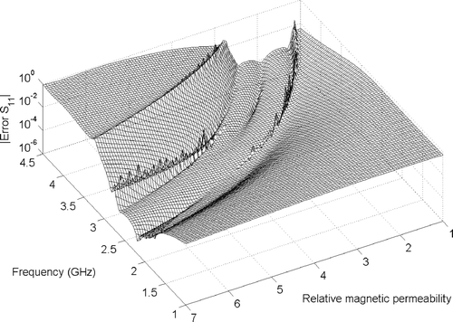
Figure 1 shows a coaxial line with toroid-shaped inset. For this simple structure, analytical solutions are easily obtained. The system response is given by the reflection coefficient S ₁₁ as a function of frequency f and inset permeability μ _r , where the parameter domain is defined by f = 1 … 4.5 GHz and μ _r  = 1 … 7. We purposely choose the expansion point at (f = 3 GHz, μ _r  = 4), such that there is no reflection at all and construct a ROM of order q = 10. Since the structure is a two-port device, the resulting ROM is of dimension 2 · (q + 1) · (q + 2)/2 = 132. Figure 2 depicts the response surface for |S ₁₁|, sampled by 201 × 201 = 40401 points. The CPU-time for computing all 40401 ROM solutions on a 2.2 GHz Pentium IV processor is less than 200 s, whereas the same number of full FE simulations would take 258 h. Figure 3 gives the magnitude of the error in reflection coefficient |Error S ₁₁|,

where the analytical solution is taken as the reference . It can be seen that the error is typically in the order of 10⁻⁴ and increases to 10⁻² in the vicinity of (f = 4.5 GHz, μ _r  = 7), where the resolution of the FE mesh is worst. For comparison with previous methods, we have constructed a model of the same dimension by direct implementation of (10) followed by an orthogonalization step after the building process. The error plot of Figure 4 shows that these results are far off.

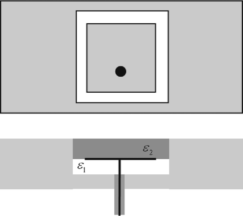
Figure 1. Coaxial probe. Geometry and material data. All dimensions are in millimetres.

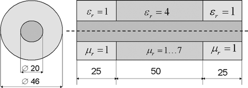
Figure 2. Coaxial probe. Magnitude of reflection coefficient as a function of frequency and relative permeability, as computed by the proposed algorithm.

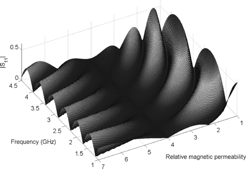
Figure 3. Coaxial probe. Magnitude of error in reflection coefficient (37) as a function of frequency and relative permeability.

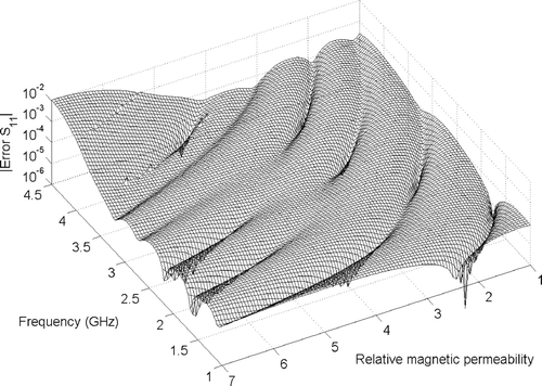
Figure 4. Coaxial probe. Magnitude of error in reflection coefficient (37) as a function of frequency and relative permeability computed by direct implementation of definition (10) and post-orthogonalization.

7.2 Multivariate polynomially parameterized system

We now consider the patch antenna of Figure 5. The system response is the reflection coefficient S ₁₁ as a function of frequency f = 3 … 8 GHz and the relative permittivity values of the two dielectrics ϵ _r1 = 1 … 5, ϵ _r2 = 1 … 3. Motivated by the authors' previous analysis of that specific design, the expansion point is chosen at (f = 6 GHz, ϵ _r1 = 4, ϵ _r2 = 2), A FE approach 22 using absorbing boundary conditions and transfinite elements 23 results in a linear system of equations of the form

Figure 5. Patch antenna. Schematic of the geometry, featuring two different dielectrics. Dimensions are given in 21.

with n = 58,247 degrees of freedom. We introduce the parameters

where denote nominal values at the expansion point. By plugging (39) into (38), we obtain the polynomially parameterized system of equations

Note that, by , terms of third degree are present. The order of the reduced model is chosen to be q = 8, and the resulting model dimension is 165. Figure 6 shows a two-dimensional cut through the three-dimensional response hyper-surface. To assess the accuracy of the ROM, we need to compute reference values by full FE runs, because analytic solutions are not available. Since such calculations are very time-consuming, we are unable to present error data for the two-dimensional cut of Figure 6. Instead, we just consider a line placed at one outer edge of the parameter domain (ϵ _r1 = 1, ϵ _r2 = 3), sampled by 51 equidistant points. The corresponding solutions and errors (37) are given in Figures 7 and 8, respectively. Again, accuracy is very satisfactory.

Figure 6. Patch antenna. Magnitude of reflection coefficient at ϵ _r2 = 3 as a function of frequency and relative permittivity ϵ _r1.

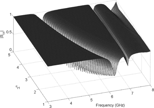
Figure 7. Patch antenna. Comparison of ROM with full FE simulations for ϵ _r1 = 1 and ϵ _r2 = 3.

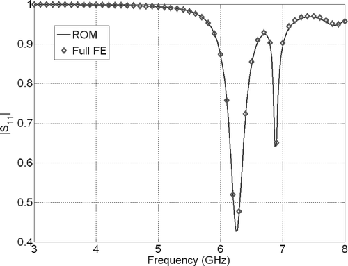
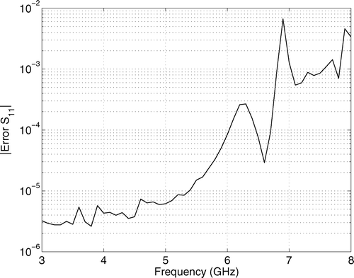
Figure 8. Patch antenna. Magnitude of error in reflection coefficient (37) as a function of frequency. Parameters ϵ _r1 = 1, ϵ _r2 = 3.

8 Summary and outlook

We have presented a general recursion for the Krylov space of polynomially parameterized systems of linear equations with parameter-dependent right-hand sides. In addition, we have proposed an algorithm for computing a well-conditioned basis and a related single-point method for the order reduction of multi-parameter systems. Numerical examples validate the reliability of the suggested approach.

At present, the order of the ROM is set by the user directly. In the future, we intend to develop an error estimator that stops the MOR process automatically as soon as a pre-defined level of accuracy is obtained. Since the model dimension grows very rapidly when the number of parameters gets large, purging strategies that reduce the number of basis vectors without sacrificing accuracy are to be developed. Another goal of future work is to build an even more powerful tool for multivariate MOR by employing the single-point algorithm presented in this paper as a building block within a multi-point framework.

Acknowledgement

V. Hill was supported by a Grant from Ansoft Corporation. P. Ingelström was supported by a fellowship from the Alexander von Humboldt-Foundation.

References

- Pillage , L. T. and Rohrer , R. A. 1990 . Asymptotic waveform evaluation for timing analysis . IEEE Trans. Comp. Aided Design Integr. Circuits , 12 : 352 – 366 .
- Chiprout , E. and Nakhla , M. 1993 . Transient waveform estimation of high-speed MCM networks using complex frequency hopping . Multi-Chip Module Conference (MCMC) . 1993 , Santa Cruz, CA, USA. pp. 134 – 139 .
- Celik , M. 1995 . Pole-zero computation in microwave circuits using multi-point Padé approximation . IEEE Trans. Circuits Syst. I , : 6 – 13 .
- Feldmann , P. and Freund , R. W. 1995 . Efficient linear circuit analysis by Padé approximation via the Lanczos process . IEEE Trans. Comp. Aided Design Integr. Circuits , 14 : 639 – 649 .
- Gallivan , K. , Grimme , E. and Van Dooren , P. 1994 . Asymptotic waveform evaluation via a Lanczos method . Appl. Math. Lett. , 7 : 75 – 80 .
- Grimme , E. Krylov projection methods for model reduction Ph.D. diss., Coordinated-Science Laboratory, University of Illinois at Urbana-Champaign, 1997
- Ruhe , A. 1984 . Rational Krylov sequence methods for eigenvalue computation . Lin. Alg. Appl. , 58 : 391 – 405 .
- Slone , R. D. and Lee , R. 2000 . Applying Padé via Lanczos to the finite element method for electromagnetic radiation problems . Radio Science , 35 : 331 – 340 .
- Salimbahrami , B. and Lohmann , B. 2006 . Order reduction of large scale second order systems using Krylov subspace methods . Linear Algebra Appl. , 415 : 385 – 405 .
- Su , T. J. and Craig , R. R. Jr. 1989 . Model reduction and control of flexible structures using Krylov vectors . J. Guidance , 14 : 260 – 267 .
- Slone , R. D. , Lee , R. and Lee , J.-F. 2003 . Broadband model order reduction of polynomial matrix equations using single-point well-conditioned asymptotic waveform evaluation: derivations and theory . Int. J. Numer. Meth. Eng. , 58 : 2325 – 2342 .
- Bai , Z. and Su , Y. 2005 . Dimension reduction of second-order dynamical systems via a second-order Arnoldi method . SIAM J. Sci. Comput. , 26 : 1692 – 1709 .
- Gunupudi , P. , Khazaka , R. and Nakhla , M. 2002 . Analysis of transmission line circuits using multidimensional model reduction techniques . IEEE Trans. Adv. Packaging , 25 : 174 – 180 .
- Weile , D. S. 1999 . A method for generating rational interpolant reduced order models of two-parameter linear systems . Appl. Math. Lett. , 12 : 93 – 102 .
- Daniel , L. 2004 . A multiparameter moment-matching model-reduction approach for generating geometrically parameterized interconnect performance models . IEEE Trans. Comp. Aided Design Integr. Circuits , 23 : 678 – 693 .
- Weile , D. S. and Michielssen , E. 2001 . Analysis of frequency selective surfaces using two-parameter generalized rational Krylov model-order reduction . IEEE Trans. Antennas Propagat. , 49 : 1539 – 1549 .
- Codecasa , L. 2005 . A novel approach for generating boundary condition independent compact dynamic thermal networks of packages . IEEE Trans. Compon. Packaging , 28 : 593 – 604 .
- Odabasioglu , A. , Celik , M. and Pileggi , L. T. 1998 . PRIMA: passive reduced-order interconnect macromodeling algorithm . IEEE Trans. Comp. Aided Design Integr. Circuits , 17 : 645 – 654 .
- R.W. Freund, Passive reduced-order modeling via Krylov subspace methods, Numerical Analysis Manuscript No. 00-3-02, (2000). Available at http://cm.belllabs. com/cs/doc/00
- Boley , D. L. 1994 . Krylov space methods on state-space control models . Circuits Syst. Signal Process , 13 : 733 – 758 .
- González de Aza , M. 1998 . Full-wave analysis of cavity-backed and probe-fed microstrip patch arrays by a hybrid mode-matching generalized scattering matrix and finite-element method . IEEE Trans. Antennas Propagat. , 46 : 234 – 242 .
- Bossavit , A. and Mayergoyz , I. 1989 . Edge-elements for scattering problems . IEEE Trans. Magn. , 25 : 2816 – 2821 .
- Cendes , Z. J. and Lee , J.-F. 1988 . The transfinite element method for modeling MMIC devices . IEEE Trans. Microwave Theory Tech. , 36 : 1639 – 1649 .