Comparison and combination of reduced-order modelling techniques in 3D parametrized heat transfer problems

Abstract

Reduced basis method has successfully been used in 2D to solve heat transfer parametrized problems. In this work, we present some 3D applications in the same field. We consider two problems, the steady Thermal Fin and the time-dependent Graetz Flow, we compare two reduced-order modelling techniques: Reduced basis and Proper orthogonal decomposition, then we apply a combination of the two strategies in the time-dependent case.

Keywords:

• reduced basis method
• reduced order modelling
• proper orthogonal decomposition
• heat transfer
• Graetz flow
• parametrized partial differential equations
• a posteriori error bounds
• greedy algorithm

1. Introduction

Computing the solution of partial differential equations (PDEs) is very expensive. For realistic simulations, we need thousands of degrees of freedom to obtain good approximations of the solution. For example, for the analysis and the optimization of an engineering system, we have to compute several solutions of the PDEs. We may be interested in outputs depending on the state solution: that is, maximum or average temperature, heat transfer rates, flow rates and so on. The introduction of some parameters leads to input–output relationships. The input parameter may represent boundary conditions and sources, geometric configurations or physical properties. Classical discretization methods such as finite element (FE), finite volume or spectral methods are not the most appropriate. Consequently, we have to develop techniques that reduce the cost and time of the computations. These techniques are called reduced-order methods (ROMs). The reduced basis (RB) method is one of them and is indicated to evaluate very quickly the outputs mentioned earlier. ¹ Moreover, the goal of the RB method is to reduce the complexity of a system without loss of information or the accuracy of the results. This method does not replace any discretization method, such as the FE method, but there is a collaboration with it. The idea is to start with some selected FE solutions, each of them of dimension , due to the nodal discretization and then to construct a RB space made up of just N of these basis functions, where . The RB method is particularly well suited in two contexts: the real-time context and the many-query context. The real-time context arises in applications such as control engineering and in parameter estimations. The many-query context is involved in multiscale, multiphysics and optimization problems.

In this work, we essentially treat affine coercive elliptic problems [4]. The affine parameter-dependence hypothesis enables an efficient Offline–Online computation. The RB method reduces notably the Online cost providing much effort and preparation in the Offline step. So, this method is optimized for problems that allow rapid Online computation at the cost of a bigger Offline effort, because the Offline part depends on , whereas the Online part depends only on N.

In this work, we will use the RB method to solve 3D conduction and convection problems: the steady thermal fin problem and the time-dependent Graetz flow problem.

In this article, we are more interested in extending results about convergence and computational time for the RB method applied to 3D problems focusing on heat transfer, both steady and time dependent, problems to show that the RB method can also be used for more complex settings. Very recent works dealing with 3D steady applications by the RB method are [4] with a linear elasticity block and [5] with an electromagnetic scattering problem.

In the following section, we will review the main ingredients of the RB method for affine coercive elliptic problems and a sampling strategy. We will treat the geometric variations and the constructions of affine mappings, then we recall the a posteriori error bounds.

Section 3 is the continuation of the previous one, where we extend our attention to parabolic problems. We will introduce the main changes arising with the time dependency.

In Section 4, we present the steady 3D thermal fin problem (see [6–8]), which is a steady heat conduction problem with parametrized geometry and physics, previously solved in the 2D case (see [9]). We will give a description of the problem and its mathematical formulation, and we present some convergence results for the RB method and a comparison with another ROM technique: Proper Orthogonal Decomposition (POD). The behaviour of the parametrized output is discussed too.

In Section 5, we solve the time-dependent Graetz flow problem (see [7,10,11]), modelling heat conduction and forced heat convection in a duct. As done for the thermal fin, we will introduce the mathematical description of the problem and some numerical results by solving the problem with the RB method.

2. Overview of the RB method for elliptic problems

We will present the RB methodology for compliant, coercive affine elliptic problem after giving the exact formulation (in weak form) of the problem and building upon an FE discretization. The last part deals with the construction of a posteriori error bounds. For more details, see [4] and [1].

2.1 Elliptic coercive parametric PDEs: compliant case

2.1.1 Exact problem formulation

Let , be a suitable physical domain with Lipschitz continuous boundary . Let the parameter domain. Let be a Hilbert function space such that where () for a scalar (vector) field. Here, and We associate to an inner product and a norm equivalent to the -norm denoted by and , respectively, whose definitions will be given below. Let be a continuous coercive parametric bilinear form. Let f be a continuous parametric linear functional. We consider the following problem: given , evaluate , where satisfies

(1)

The superscript ^e refers to exact. Here is the input parameter, the scalar output, the linear output functional and the field variable. Under the hypothesis on the forms a and f, the problem (1) has a unique solution. Moreover, we assume that f and are bounded over and that we have the following affine developments

(2)

(3)

for finite and relatively small , respectively. We consider that the for , are simple algebraic expressions that can be readily evaluated in operations. Till the end of this section, we will consider compliant problems, that is, we assume that (1) a is symmetric and (2) for simplicity. ²

2.1.2 Truth approximation

We introduce the truth approximation upon which we will construct the RB approximation. Moreover, we will measure the error in the RB approximation relative to this truth approximation (see Section 2.4).

We now consider the space such that , and we take the Galerkin projection: given , evaluate , where satisfies Typically, we take large to obtain very small. Then, the RB will be built on this truth approximation. For , we define the energy inner product and the energy norm, respectively, as and Moreover, for a given , we define the -inner product and the -norm for , respectively, as and where is a non-negative real parameter and . As , the inner products and the norms defined above are the same for the space . ³ Now, we can define precisely the exact and discretized coercivity constants, respectively, as

From the coercivity hypothesis, we have that , , and from hypothesis on (conforming space), we have that , . In the same way, the continuity constants are defined as

where is finite for all and , for all .

2.1.3 RB approximation

The RB approximation is a Galerkin projection on a N-dimensional approximation space that focuses on a low-dimensional, smooth, parametric manifold , induced by the parametric dependence. The space is too general because it approximates all members of . So to approximate a solution , it is sufficient to be able to approximate only functions in . The idea is to choose and compute N basis functions called snapshots, and then for an arbitrary value , compute the solution associated to this parameter (denoted ) by a linear combinations of , . More precisely, let be an integer, for , let be a N-dimensional subspace of . We assume that these spaces satisfy the nested or hierarchical condition, that is,

(4)

The condition (4) is very important for efficiency and for reducing the computational cost. There are several spaces that satisfy the hierarchical solution, for example Taylor spaces, Lagrange–Hermite spaces and POD spaces [1,4]. In this work, we will focus on Lagrange spaces and POD spaces. These spaces will be introduced later (see Section 2.2). Now, we consider the Galerkin projection to obtain our RB approximation: given , evaluate where satisfies

(5)

From coercivity and continuity hypothesis on a and f, our conforming RB , problem (5) admits a unique solution. Moreover, we can demonstrate the well-known Galerkin optimality results [1]:

Proposition 2.1: For any and and satisfying (5)

(6)

(7)

and furthermore for the output (square effect):

(8)

as well as

(9)

2.2 Sample/space assembling strategies

We recall two sampling strategies to obtain the RB spaces. The first one is the POD and the latter is the Greedy Lagrange algorithm. In Section 4.4.1 of this work, we will compare these two strategies with some examples.

Let be a finite sample set called test sample of parameters in . These parameters are often chosen by Monte Carlo methods with respect to a uniform or log-uniform density. We assume that the cardinality of is very large to cover all the set . Now, we define the following norms: properly for a function , and

For a function (or ) we then define in the same way, and

2.2.1 POD RB spaces

The POD approach ([12]) is popular most notably in time-domain reduced-order modelling (see [13]). This technique can also be applied within the parametric context, as we now describe (see [1]).

Given , we define the POD RB spaces as the solution of the optimization problem

(10)

where refers to the orthogonal projection in the X-inner product. Now, we define the correlation matrix given by

(11)

If we express as and if we define the vector and the matrix such that we have that We then solve the following eigenproblem: find , , such that

(12)

Arranging the eigenvalues in descending order , we define , , as

We take as the smallest N such that

We then construct the POD RB spaces as We then take as our RB space for the choice , .

To use a POD approach, we have to compute all solutions for all . The most expensive part is the construction of the correlation matrix and then the resolution of several eigenproblems (12), but POD is very useful for some small and that is the reason why it is used in time-dependent applications.

2.2.2 Greedy Lagrange spaces

The idea of this strategy is starting with a to select N parameters and to form the RB space (see [14]). For the Greedy approach, we need a sharp, rigorous and efficient bound for the RB error , where is the RB approximation associated with the space . We now present the Greedy algorithm. We define an upper bound for , a tolerance of the error. Given , and ,

With POD, we have to compute the snapshots for all ; here we only have to compute snapshots. In this strategy, we use a posteriori error bound to approximate the expensive true error . ⁴

2.3 Geometric variations

If we want to consider geometric variations of the domain, we have to assume that the reference domain is the pre-image of the parameter-dependent original domain . For more details, the reader can refer to [4]. We shall assume that for all in , we have a domain decomposition of ,

(13)

where the , is mutually non-overlapping open subdomains,

(14)

This coarse domain decomposition will be denoted RB triangulation. We now choose a value and define our reference domain as . It is easy to see that and We will build a very fine FE subtriangulation of the RB triangulation of . This FE subtriangulation ensures that the FE approximation accurately treats the perhaps discontinuous coefficients (arising from property and geometry variations) associated with the different subdomains and the subtriangulation also plays an important role in the generation of our affine representation (3). We emphasize that only affects the accuracy of the underlying FE approximation upon which the RB discretization and a posteriori error estimator are built.

A necessary condition for the affine representation (3) is the so called affine geometry precondition. This condition says that for any original domain that admits a domain decomposition (13), there exists affine mappings : , , that are (1) individually bijective and (2) collectively continuous, that is,

(15)

and such that

(16)

We now define our (bijective) affine mappings more explicitly: for , any in and any ,

(17)

for given : and : . We can then define the associated Jacobians

(18)

where det denotes the determinant. Note that the Jacobian is constant in space over each subdomain. We further define, for any ,

(19)

this matrix shall prove convenient in subsequent derivative transformations.

We may interpret our local mappings in terms of a global transformation. In particular, for any , the local mappings 16 induce a global bijective piecewise-affine transformation : : for any ,

(20)

note that the one-to-one property of this mapping (and, hence the arbitrariness of our min choice in Equation (20)(20) is ensured by the interface condition (15).

2.3.1 Affine mappings: single subdomain

As we consider a single subdomain in this section, we shall suppress the subdomain superscript for clarity of exposition. We shall focus on the 3D case . The 2D case is detailed in [4]. The affine transformation (17) can be rewritten as

(21)

we shall refer to and as the mapping coefficients. In this case, we have 12 mapping coefficients that entirely define the affine transformation (21). Under our assumption that the mapping is invertible, we know that our Jacobian, of (18), is strictly positive and that the derivative transformation matrix, of Equation (19)(19), is well defined.

The mapping coefficient can be identified by the relationship between four non-coplanar pre-image points or nodes, in Ω and four parametrized image nodes, , in . In particular, for given , application of Equation (21)(21) to the selected nodes yields

(22)

Equation (22)(22) constitutes 12 independent equations by which to determine the 12 mapping coefficients. To be more explicit in our construction, we first form the matrix (more generally, ) as

We further introduce the vector of image nodal locations as . We then obtain our affine mappings

To illustrate how the parametric dependence propagates from the (desired) parametrized domain to the mapping coefficients, we give the example of a tetrahedra. We note that parallelepipeds are the most intuitive subdomains to be able to build transformations by hand, invoking the usual translation, dilation, rotation and shear primitives. However, we can state a parallelism with the 2D case and consider curvy tetrahedra instead of triangle and curvy triangle. Here, we shall thus focus only on tetrahedra-building blocks. Suppose a tetrahedra as in Figure 1(a) with vertices and that are pre-images nodes of points and (Figure 1(b)). The reference domain and the original domain are, respectively, denoted by and . The pre-images nodes correspond to the image node for a particular value of the parameter. Here, , that is,

Figure 1. Variation on a tetrahedra. (a) Reference domain . (b) Original domain .

Consequently, we have that and It follows that

2.4 A posteriori error bound

A posteriori error bounds for the RB approximation are crucial for both efficiency and reliability. With regard to efficiency, error bounds play a role in Offline and Online computational stages. In the Greedy algorithm, for example, the application of error bounds permits larger training sample at reduced Offline computational cost. Hence, we have a better accuracy of the RB approximation that can be obtained with a smaller number N of basis functions, and hence we have a reduced Online cost: a posteriori error estimation permits us to control the error, which in turn permits us to minimize the computational effort (see [1]). With regard to reliability, our Offline sampling procedures can not be exhaustive. For a large number of parameters P, there is a large portion of the parameter space that remains unexplored. So, the error of a large part of our parameter domain may be uncharacterized. The a posteriori error bounds permit to bound the error for all new parameter value . We can be sure that constraints are satisfied, feasibility conditions are verified and prognoses are valid (in each case not only for the RB approximation but for the truth FE solution). So we do not loose any confidence in the solution compared with the underlying FE solution while exploiting the rapid predictive power of the RB approximation (see [4]). ⁷

2.4.1 Error bounds

We define the residual as

(23)

where is the dual space of . We also introduce the function , the Riesz representation of

(24)

Introducing the error , we have from Equations (24)(24) and (23) that

We still introduce the dual norm Note that the second equality follows from the Riesz representation theorem. This definition through the Riesz representation is crucial for the Offline–Online procedure that is developed below.

We introduce a lower bound for , that is, a function such that , and such that the evaluation is independent of . ⁸

We define now the energy, the output and the relative output error bound estimators [1], respectively, as

We introduce also the respective effectivities as a measure of the quality of the estimators

The following proposition shows that these estimators are rigorous and sharp [14].

Proposition 2.2: For ,

3. Overview of the RB method for parabolic problems

In this section, we recall linear parabolic problems. We focus only on the primal problem, ⁹ see also [13,15]. The time domain shall be denoted by where is the final time.

3.1 RB and a posteriori error bound

We introduce the weak form of the -parametrized linear parabolic PDE: given , evaluate where satisfies

(25)

with initial condition , where is bilinear, -continuous and coercive, bilinear, -continuous and coercive and linear bounded. The output functional is linear and bounded whereas is a control input. Moreover, the forms a, m, f and are affine in , as Equation (3)(3) and also m and such that and We now discretize the problem (25) in space (FE) and in time using an Euler backward discretization. We introduce as the time step and as the number of time steps. We still define , , and . Then, we obtain the discretized problem: given , , , evaluate where satisfies with initial condition , where is the -projection of . Here, and .

The theory we introduced for elliptic problem can be used for the parabolic case. More precisely, we can express our problem in a parameter-independent domain using affine mappings (Section 2.3) and we perform an RB approximation (Section 2.1.3). Then, we obtain the reduced problem: , evaluate , where satisfies , and, as in the elliptic case, we compute . We define two a posteriori error bounds and as in [15]:

(26)

(27)

where and is the residual defined as

, . Then, we have the rigorous and sharp result.

Proposition 3.1: For all and for all ,

(28)

where and are two constants. Moreover,

(29)

The idea for the construction of the space is to consider the set K as a small (time-)parameter sample and the set the space-parameter sample (Section 2.2), and to combine POD in time (Section 2.2.1) and the Greedy algorithm (Section 2.2.2) in the parameter space to set a POD–GREEDY sampling procedure (see [13]). In the next section, we will explain this strategy in details.

3.2 POD(t)–GREEDY(μ) sampling procedure

The algorithm, briefly recalled here, is composed of two stages of POD and one stage of Greedy. A previous one-stage POD–GREEDY combination has been proposed in [17]. As mentioned before, the POD is used in time whereas the Greedy is used in the parameter space. ¹⁰ We recall that, given L elements , the POD returns M -orthogonal functions such that is optimal in the sense that

For simplicity, we will write The second stage allows us to further reduce the dimension of the approximation space after the first POD in time for a fixed value of the parameter. We introduce the parameter sample and an initial parameter and set . We give now the algorithm:

Set . ¹¹ Usually we set , see [13, 15].

4. The 3D steady thermal fin problem

This section is dedicated to the resolution of a steady thermal fin problem (see [6,7]). This problem has already been solved in the 2D case in [8,9] (see also http://augustine.mit.edu/workedProblems.htm). For the 3D case, we used COMSOL [18] linked with the rbMIT software [9,20] showing that the method can be used with success to also solve more complex problems.

4.1 Heat sink: problem description

This problem considers the performance of a heat sink designed for the thermal management of high-density electronic components. The main function of a heat sink is to transfer heat from an object at a higher temperature to another at a lower temperature with greater heat capacity. The heat sink comprises a base/spreader that in turn supports a number of plate fins exposed to flowing air (see Figure 2(a)). The high density of the heat sink combined with its large area, due to fins, results in the rapid transfer of thermal energy to the surrounding cooler material. Then, the heat sink is cooled and whatever is in direct contact with it is also cooled. In our analysis, we shall consider one half of a single fin for reasons of symmetry (see Figure 2(b), [7,8]). We model the flowing air through a simple convection heat transfer coefficient. Our interest is in the temperature at the base of the spreader.

Figure 2. (a) Heat sink. (b) Respective domain for a periodic heat sink.

From the engineering point of view, this problem illustrates the application of conduction analysis to an important class of cooling problems: electronic components and systems. Examples of systems that require a heat sink to reduce their temperature are microprocessors and refrigeration.

4.1.1 Parametrized geometry and parameters

We introduce the different quantities that describe our problem. The quantities with a tilde approximately correspond to dimensional quantities and the absence of a tilde denotes non-dimensional quantities.

We assume that the spreader has thermal conductivity and the plate fin has thermal conductivity . The ratio of these conductivities is denoted by The distance between two fins is and the height of a fin is denoted by . We characterize the heat transfer from the fin to the air by a heat transfer coefficient . We consider parameters, two of them are physical and one is geometrical. The first physical parameter is the Biot number defined as The second parameter is the non-dimensional fin height, whereas the third one is given by the conductivity ratio The parameter domain is given by . We denote by the vector of parameters, that is,

The temperature is measured relative to the temperature of the air at infinity, , and non-dimensionalized with respect to , where is the dimensional heat flux into the spreader. We identify in Figure 3 the points defining the geometry and the different subdomains , , considered. We define the global domain as . As we have only one geometrical parameter, , and as is parameter independent, we can write .

Figure 3. (a) Parametrized geometry. (b) Domain boundaries.

4.2 Mathematical formulation

The non-dimensional temperature satisfies the conduction equation in . We impose continuity of temperature and heat flux at the spreader–fin interface. Moreover, we impose zero heat flux on the horizontal exposed surfaces of the spreader and fin; uniform heat flux on the spreader base and heat transfer convection (Robin) boundary conditions on the vertical face of the fin, the one exposed to the flowing air. Mathematically, satisfies

where denotes the unit outward normal. On , we impose continuity of temperature and heat flux. The output of interest is which represents the average of the temperature on the base of the spreader. ¹² In this scalar problem, we take . The weak formulation reads as follows: for all , find such that

(28)

Introducing the bilinear form and the linear functional we can rewrite Equation (30)(28) as follows: find such that

The coercivity and the continuity of the bilinear form and the continuity of the functional can be proved. So the Lax–Milgram theorem ensures the existence and unicity of the solution (see [19]).

4.3 Reference geometry

To obtain the affine decomposition of the bilinear form and to work with parameter-independent geometry. We take as reference parameter vector (see Section 2.1.2). Then, the reference domain will be . Note that we have where and . We want to construct an affine mapping , with . We remind that these mappings have to be individually bijective, collectively continuous and each mapping has the general form for given and , (see (15)).

As does not depend on any parameters, we have that where is the identity operator, . To construct , we choose four non-colinear points in and four parametrized image nodes in . Then, we apply the method developed in Section 2.3 and we obtain

4.3.1 Affine decomposition

To find the affine decomposition, we start to compute the Jacobian and the matrix , . For , all these quantities are trivial, that is, and , where is the identity matrix. For , we easily compute

We obtain the bilinear form expressed in the reference domain :

4.4 Results and visualizations

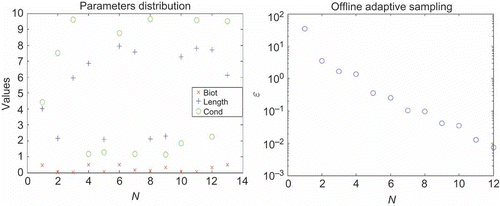
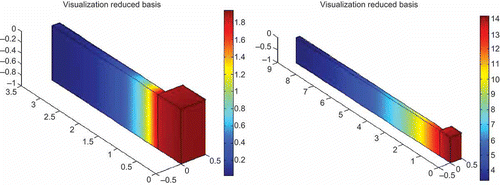
In this section, we give the convergence result of the Greedy algorithm (Section 2.2.2). Here, the sample size is , the tolerance and the . In the Figure 4(a), we have represented for each N the parameter chosen automatically by the algorithm. We have obtained for the primal problem. In the Figure 4(b), we represent the error bound for . We report in Figure 5 the visualization of some representative RB solutions.

Figure 4. Sample and error bound for the Greedy. (a) Chosen parameters. (b) Error bound . Cond denotes thermal conductivity.

Figure 5. Examples of representative solutions for (a) . (b) .

4.4.1 Comparison between the POD and the Greedy

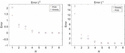
We compare the Greedy performance with that of the POD. We recall that theoretically the Greedy–RB has to minimize the RB error in -norm whereas the POD minimizes the projection error in -norm. In Figure 6(a), we represent the error in -norm for Greedy–RB and POD approximations; whereas in Figure 6(b), we represent the error in -norm.

Figure 6. Greedy and POD performance comparison. (a) . (b) .

We see that Figure 6(a) confirms the theoretical expectation, that is, the error of the Greedy–RB approximation is bigger than the error of the POD approximation because we are considering POD in its natural environment, that is, by considering -norm (and not ). The opposite is valid for POD and Greedy for smaller N in Figure 6(b) in the natural environment for the Greedy. Note that the differences are not so significant and we may consider the two approaches as equivalent (in terms of performances).

4.4.2 Output

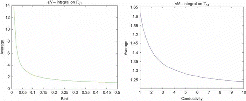
Just as non-exhaustive example, we present here the variation of the output , that is, the average of the temperature on the base of the spreader, as a function of the different parameters in 3D (see Figure 7). The error bound over the reported outputs is for all tested in the range of variation of the parameters. Graphically, the result of Figure 7(a) corresponds to results expected by the theory: if the Biot number () increases, then there is a bigger heat transfer and so the temperature at the base decreases. In Figure 7(b), we show how the temperature decreases when increases.

Figure 7. Outputs with (a) and and (b) and .

4.4.3 Computational times

We give some computational times to show the efficiency of the method. We define two kinds of computational time:

which computes the break-even, that is, the maximal number of solutions that we may evaluate with the FE method without using the RB at the same computational cost. We introduce also

where is the time we need to evaluate . This computational time shows the gain of time using the RB method for the solution of parametrized problems. We have

The break-even for . The computational costs for the RB output calculation are 150 times less expensive than the ones for the FE.

5. The 3D time-dependent Graetz problem

In this section, we will consider a 3D time-dependent non-compliant problem: the Graetz flow problem (see [7,10,11]). The 2D case has also been treated in [9] (see also http://augustine.mit.edu/workedProblems.htm).

5.1 Problem description

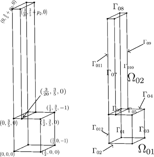
This is a classical problem in literature dealing with forced heat convection combined with heat conduction in a channel separated into two parts. The first part is made up of cold walls, whereas the second one has hot walls. The temperature at inlet is imposed and the flow has a known given convective field. In Figure 8(a), we can see the duct with the cold and hot portions. The physical domain is defined in Figure 8(b). We recall that the quantities with a tilde are dimensional quantities. A point is non-dimensionalized with respect to , the width of the channel (in the -direction). We introduce also as the dimensional conductivity coefficient for the air flowing in the channel, the dimensional diffusivity and the reference velocity for the convective field. The Péclet number is defined as . We consider three parameters . We denote by and the geometric parameters that represent the height of the cold portion and the length of the hot portion, respectively (see Figure 8(c)). The last one is the Péclet number that is a physical parameter, that is, . The parameter domain is given by .

Figure 8. (a) A channel with cold and hot portion. (b) Domain boundaries. (c) Parametrized geometry.

5.2 Mathematical formulation

The non-dimensionalized temperature ¹³ satisfies the unsteady advection–diffusion equation in . The time interval is , with T being the final time. We impose continuity of temperature and heat flux on all internal faces. At the inflow and on the cold walls, we impose homogeneous Dirichlet boundary condition. On the hot walls, we have non-homogeneous Dirichlet boundary condition and at the outflow, we impose zero heat flux (homogeneous Neumann boundary condition). ¹⁴

Mathematically, satisfies

where denotes the unit outward normal and is the control input. On , we impose continuity of temperature and heat flux. The convective field is . The output of interest is where is a function of time. This output represents the average temperature. Let us introduce the space . We will also introduce a lifting of , such that and , where . We can now give the weak formulation: for all , find such that

(29)

where

and

The function . The coercivity and the continuity of the bilinear form and the continuity of the functional can be proved. So the Lax–Milgram theorem ensures the existence and unicity of the solution (see [19]).

5.3 Reference geometry

As we did for the thermal fin, we will construct the affine mappings to obtain the affine decomposition of the bilinear forms and . In this case, the reference domain is given for , whereas the reference subdomains are , . We want to construct an affine mapping , with . In this problem, the two subdomains depend on the parameters. We apply the methodology explained in Section 2.3 for the two subdomains and we obtain

To find the affine decomposition, we compute the Jacobian and the matrix , . We obtain that

We obtain the time-independent bilinear form expressed in the reference domain:

In the same way, we obtain the time-dependent bilinear form

and the linear functional

The affine decompositions are and The quantities can easily be deduced from the definition of the forms a, m and F respectively.

5.4 Results and visualization

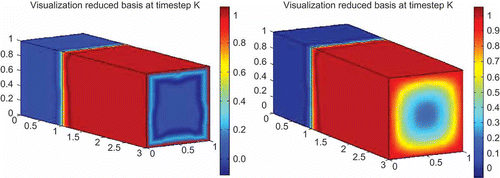
We show the results of the POD–Greedy–RB algorithm described in Section 3.2. Here, the sample size is , the tolerance and the (Section 3.2). As the problem is non-compliant, we have to do the POD–Greedy for the primal and dual problem (see [20]). In Figure 9(a) and 10(a), we have represented for each N the parameter , which was chosen by the Greedy algorithm. We have obtained for the primal problem and . In Figure 9(b) and 10(b), we represent the error bound for . In Figure 11, we represent the solution for for different timesteps and control input .

Figure 9. Samples distribution and greedy error bounds for the primal problem. (a) Chosen parameters. (b) Error bound .

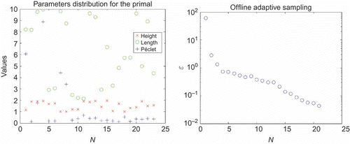
Figure 10. Sample distribution and Greedy error bound for the dual problem. (a) Chosen parameters. (b) Error bound .

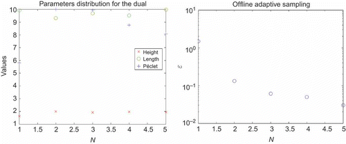
Figure 11. Example of representative solution for µ = (1, 2, 10). Visualizations at (a) t⁰ = 0, Δ^s _N = 0 and (b) t6 = 0.3, Δ^s _N = 0.0131.

5.4.1 Output

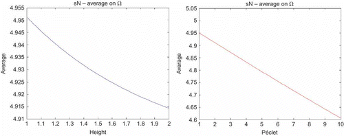
We deal with the output : the average temperature in the duct, for different parameters . For the computations, we took and timesteps, then . In Figure 12(a), we represent the evolution of the average temperature when the height of the duct increases. Figure 12(b) shows that the average temperature at decreases when the Péclet increases. Physically, if the Péclet is bigger, the transport is dominating and then the temperature is lower. The error bound over the plotted output is for all tested.

Figure 12. Outputs with (a) and (b)

5.4.2 Computational time

We consider the different computational time measurement that we defined previously in Section 4.4.3: ()

Then, if we want to compute more than 72 solutions, the use of the RB method is more efficient and recommended. Here, looking also at , we see that the use of the RB method is very gainful. We can get faster Online output evaluation (5 permil of computational costs in the Online evaluation compared with a standard FE method evaluation).

6. Conclusions

This article extends the application of the RB methods to 3D parametrized heat and mass transfer problems and a comparison/combination with another ROM technique: POD. The results show that the potentialities of the RB methodology and the computational savings are even more significant in the 3D case and with time-dependent problems, where a POD–GREEDY combined technique has been applied.

Acknowledgements

We are grateful to Professor. A. Quarteroni (EPFL) and Professor. A.T. Patera (MIT) for support, very useful remarks and suggestions and to the referees who helped in improving this manuscript with their remarks.

Notes

1. A brief historical introduction on RB can be found in [1]. Almroth, Stern and Brogan [2] studied the method for one parameter problem. Then with Noor [3] the method was extended to multi-parameter and non-linear problems in structural analysis and only later in fluid dynamics. Current research is dedicated to the development of a posteriori error estimation procedure and to the development of effective sampling strategies for many parameters spaces in order to improve convergence and computational efficiency [4].

2.We may extend the methodology to the non-compliant case with the introduction of a dual problem [4].

3. The choice of and will affect the quality and efficiency of our RB a posteriori error estimators, but will not affect directly our RB output predictions (see [4]).

4. Note that in theory, the Greedy minimizes the error in the -norm whereas the POD minimizes the projection error in -norm.

5. Note that we purposely define with respect to the exact problem, rather than the FE approximation: cannot depend on (to be meaningful).

6. Note that is non-singular under our hypothesis of non-coplanar pre-image nodes and independent of μ; the parametric dependence derives from .

7. The a posteriori error bound must be rigorous (greater or equal to the true error) for all N and all parameters values in the parameter domain . Non-rigorous error indicators may suffice for adaptivity, but not for reliability. Second, the bound must be reasonably sharp. An overly conservative error bound can yield inefficient approximations, typically for N too large. Third, we require efficiency, that is, the cost of the Online evaluation and storage must be independent and should be comparable to the cost of the RB output prediction (see [1]).

8. The is computed by the Successive Constraint Method (SCM) that is an algorithm to construct lower bounds for the coercivity (and in the non-coercive case, inf–sup stability) constant. This method is based on an Offline–Online computational procedure too and it reduces considerably the Online calculation effort. We will not present the method, but the reader can refer to [4,14].

9. A primal-dual formulation is possible to consider non-compliant outputs [16].

10. In this section, we will omit the superscript for the RB approximations.

11. Note that the complexity remains and is not . The Greedy selects parameter and then we have to compute all the state solution for and apply the POD procedure. Then, the second POD procedure gives us spaces of dimension N.

12. By taking into account the symmetry of the fin configuration, we just consider a half of the fin.

13. For convenience, we will not indicate the -dependence of , that is, we will write as .

14. The homogeneous Dirichlet boundaries will be denoted by that is, and the non-homogeneous Dirichlet boundary will be denoted by , that is, . We denote . The Neumann boundary will be denoted by .

References

- Patera , A.T. and Rozza , G. 2006–2011 . Reduced Basis Approximation and A Posteriori Error Estimation for Parametrized Partial Differential Equations , To appear in MIT Pappalardo Graduate Monographs in Mechanical Engineering, © MIT . Version 1.0
- Almorth , B.O. , Stern , P. and Brogan , F.A. 1978 . Automatic choice of global shape functions in struc-tural analysis . AIAA Journal , 16 : 525 – 528 .
- Noor , A.K. and Peters , J.M. 1980 . Reduced basis technique for nonlinear system analysis of structures . AIAA Journal , 18 ( 4 ) : 455 – 462 .
- Rozza , G. , Huynh , D.B.P. and Patera , A.T. 2008 . Reduced basis approximation and a posteriori error estimation for affinely parametrized elliptic coercive partial differential equations: application to transport and continuum mechanics . Arch. Comput. Meth. Eng. , 15 ( 3 ) : 229 – 275 .
- Pomplun , J. and Schmidt , F. Accelerated a posteriori error estimation for reduced basis method with application to 3D electromagnetic scattering problems . SIAM J. Sci. Comp. , 32 ( 2010 ) 498 – 520 .
- Arpaci , V.S. 1966 . Conduction Heat Transfer Addison-Wesley, Reading
- Incropera , F. , Dewitt , D. , Bergmann , T. and Lavine , A. 2007 . Fundamentals of Heat and Mass Transfer , John Wiley & Sons, New York .
- Rozza , G. , Huynh , D.B.P. , Nguyen , N.C. and Patera , A.T. 2009 . Real-Time Reliable Simulation of Heat Transfer Phenomena, ASME Summer Heat Transfer Conference, Proceedings, San Francisco , CA : Paper . HT2009-88212
- Reduced Basis at MIT (2009). http://augustine.mit.edu/methodology.htm, (http://augustine.mit.edu/methodology.htm,)
- Arpaci , V.S. and Larsen , P.S. 1984 . Convection Heat Transfer , NJ : Prentice Hall, Englewood Cliffs .
- Rozza , G. , Nguyen , N.C. , Patera , A.T. and Deparis , S. 2009 . Reduced basis method and a posteriori error estimators for heat transfer problems , CA : ASME Summer Heat Transfer Conference, Proceedings, San Francisco . Paper HT2009-88211
- Holmes , P. , Lumley , J.L. and Berkooz , G. 1996 . Turbulence, Coherent Structures, Dynamical Systems and Symmetry , Cambridge : Cambridge University Press .
- Nguyen , N.C. , Rozza , G. and Patera , A.T. 2009 . Reduced basis approximation and a posteriori error estimation for the time-dependent viscous Burgers' equation . Calcolo , 46 ( 3 ) : 157 – 185 .
- Huynh , D.B.P. , Rozza , G. , Sen , S. and Patera , A.T. 2007 . A successive constraint linear optimization method for lower bounds of parametric coercivity and inf-sup stability constants . Comptes Rendus Mathematique , 345 : 3362 – 3366 .
- Nguyen , N.C. , Rozza , G. , Huynh , D.B.P. and Patera , A.T. 2010 . “ Reduced basis approximation and a posteriori error estimation for parametrized parabolic PDEs; application to real-time Bayesian parameter estimation ” . In Computational Methods for Large Scale Inverse Problems and Quantification of Uncertainty , Edited by: Tenorio , L. , van Bloemen Waanders , B. , Mallick , B. , Willcox , K. , Biegler , L. , Biros , G. , Ghattas , O. , Heinkenschloss , M. , Keyes , D. and Marzouk , Y. 151 – 173 . Chichester : John Wiley & Sons .
- Grepl and , M. and Patera , A.T. 2005 . A posteriori error bounds for reduced basis approximations of parametrized parabolic partial differential equations . Math. Model. Numer. Anal. , 39 ( 1 ) : 157 – 181 .
- Haasdonk , B. and Ohlberger , M. 2008 . Reduced basis method for finite volume approximations of parametrized linear evolution equations . Math. Model. Numer. Anal. , 42 ( 2 ) : 277 – 302 .
- Comsol Multiphysics 3:5a. Guide http://math.nju.edu.cn/help/mathhpc/document.htm (http://math.nju.edu.cn/help/mathhpc/document.htm)
- Quarteroni , A. 2009 . Numerical Models for Differential Problems, MS&A, Volume 2 , Springer, Milan .
- D.B.P. Huynh, N.C. Nguyen, G. Rozza, and A.T. Patera, Documentation for rbMIT Soft-ware: I. Reduced Basis (RB) for Dummies, II. Time dependent problems, © MIT. http://augustine.mit.edu, (http://augustine.mit.edu,)