Reduced basis approximation and a posteriori error estimates for a multiscale liquid crystal model

Abstract

We present a reduced basis framework and associated a posteriori error estimates for the multiscale Stokes Fokker–Planck system that governs the flow of a dilute suspension of rod-like molecules immersed in a Newtonian solvent, relevant in liquid crystals modelling. The Fokker–Planck equation dictates the microscale behaviour and must be solved at every quadrature point of the macroscale finite element mesh – this is a natural example of a many-query problem for which the certified reduced basis method is well suited. We focus on a Poiseuille flow problem to simplify the presentation of ideas, but we note that the methods developed in this article generalize directly to more complicated problems. Numerical results demonstrate that our reduced basis approach leads to significant computational savings and also that our error estimator performs well for moderate parameter values.

Keywords:

• multiscale modelling
• liquid crystals
• Fokker–Planck equation
• certified reduced basis
• a posteriori error bounds

1. Introduction

We are interested in simulating the flow of dilute liquid crystal suspensions. A standard approach to modelling this type of system is to represent the suspension as an ensemble of non-interacting microscopic rod-like dumbbells immersed in a Newtonian solvent – here, a dumbbell refers to two masses connected by an inflexible rod. From this mechanical description, the multiscale Doi model [1] can be derived, which couples a microscopic Fokker–Planck equation posed on a configuration space (the space of possible configurations of a dumbbell, i.e. a sphere) with a macroscopic Stokes equation posed on physical space (the macroscopic fluid domain). In this context, the Stokes equation describes the flow of the macroscopic Newtonian solvent and contains an ‘extra-stress’ forcing term that accounts for the non-Newtonian contribution of the liquid crystal molecules to the flow. The liquid crystal extra-stress can then be evaluated through a weighted ensemble average of the dumbbell orientations at a given point in the macroscopic domain [2,3].

We note that in the study of liquid crystals, the primary focus is generally on concentrated regimes in which collective dynamical phenomena such as tumbling and kayaking occur. Concentrated regimes can be modelled through a non-linear Fokker–Planck model that accounts for dumbbell interactions and excluded volume effects. However, the focus of this article is to propose and analyse a new numerical scheme for the Stokes Fokker–Planck system, and for this reason we restrict ourselves to the dilute case in which the Fokker–Planck equation is linear as this greatly simplifies the error analysis – extending the methodologies proposed in this article to non-dilute regimes will be a focus of future research.

The Stokes Fokker–Planck system is an interesting and important example of a fully coupled multiscale system: Stokes provides partial differential equation (PDE) coefficients (convection coefficients, to be precise) to Fokker–Planck at every point in the macroscopic domain, and Fokker–Planck provides a forcing term to Stokes. Indeed, the Fokker–Planck equation must be solved at every point (or, in the case of a finite element discretization, at every quadrature point) in the macroscopic domain. In a computational context, this is typically an onerous task as the mesh for the macroscopic domain may contain a large number of quadrature points. Nevertheless, this ‘direct PDE approach’ has been used successfully in a number of papers [3–7] – in particular, in [7] a large-scale channel flow problem with roughly 70,000 quadrature points (for a related micro–macro model of a suspension of spring-like polymers) was treated, although this computation was feasible only on a supercomputer. A more popular alternative is to employ stochastic methods by exploiting the equivalence between the Fokker–Planck equation and a stochastic differential equation [8–11]. However, the stochastic approach also has some significant limitations – most obviously slowly decaying stochastic noise is introduced into the numerical scheme, although variance reduction techniques [12–14] can at least partially address this issue.

In this article, we employ the certified reduced basis (RB) method within the context of the Stokes Fokker–Planck system to significantly reduce the computational effort required by the direct PDE approach and hence to mitigate its main drawback. We also derive a posteriori error estimators to allow us to quantify the magnitude of the error introduced by the model reduction process. We note that our error analysis for the coupled multiscale Stokes Fokker–Planck system is novel in the sense that we account for the ‘feedback’ effect due to the interplay between the two scales and we note that this approach may also be applicable to other multiscale problems.

Model reduction for the Fokker–Planck equation has received a lot of attention recently. For example, a reduced basis method was employed in conjunction with stochastic methodology in [12] as a variance reduction technique. Also, the Proper Generalized Decomposition (PGD) has been used successfully for a number of problems in computational rheology [15–17], and in particular has been able to handle especially challenging cases with high-dimensional configuration space in which microscale polymers are modelled as chains of dumbbells. The primary distinction of our methodology compared with the PGD approach is that we develop error bounds and hence, in contrast to the PGD, we are able to certify the accuracy of our reduced order model. In this article, we modify and extend the methodology from [18] in which a certified reduced basis framework was developed for the isolated (i.e. decoupled from Stokes) Fokker–Planck equation for elastic dumbbells. We develop a reduced basis numerical framework for the Stokes Fokker–Planck Poiseuille flow problem for rigid-rod dumbbells and develop error bounds for this coupled multiscale system.

The layout of this article is as follows. In Section 2, we introduce the governing equations for the micro–macro system as well as the corresponding discrete ‘truth’ finite element discretization. In Section 3, we introduce a certified reduced basis scheme for the isolated Fokker–Planck equation for rigid-rod dumbbells – this formulation follows directly from [18]. We also define a corresponding reduced basis scheme for the coupled Stokes Fokker–Planck system and a POD–Greedy algorithm to efficiently solve the reduced coupled system. In Section 4, we derive an a posteriori estimator for the error in the reduced basis macroscopic velocity field with respect to the truth velocity. Numerical results are presented in Section 5 and we close with conclusions in Section 6.

2. The micro–macro model for rod-like molecules in Poiseuille flow

We begin in Section 2.1 with the continuous formulation of the coupled Stokes Fokker–Planck system for the special case of Poiseuille flow, then in Section 2.2 we introduce a temporally and spatially discrete ‘truth’ coupled formulation. The truth formulation in Section 2.2 is the departure point for the model reduction in subsequent sections.

We note that the Poisseuille flow problem introduced below is a highly simplified model problem and, in particular, has parallel streamlines so that transport of polymer molecules within can be neglected. ¹ Nevertheless, this model problem is an appropriate focus for this article because it presents the two main challenges that we aim to treat with our RB scheme: it requires the solution of a large number of microscale Fokker–Planck equations (and is therefore computationally expensive) and also exhibits the micro–macro coupling that is a challenge from the point of view of error analysis.

2.1. Continuous formulation of the micro–macro system

Let us consider Poiseuille flow in the domain . Given a constant pressure gradient and a coupling constant that determines the strength of the rod-like molecules' contribution to the macroscopic fluid stress, the Stokes equation for macroscopic velocity field reduces to a Poisson problem in this one-dimensional case and we obtain

(1)

for . Note that here we consider the zero Reynolds number limit, in which case the temporal derivative vanishes. In Equation (1)(1), is the non-Newtonian extra-stress obtained from the solution of the Fokker–Planck equation, . More precisely, assuming the rigid-rod dumbbells are sufficiently dilute so that they do not interact with one another (but only interact with solvent molecules) then (where D is the unit sphere, , in ) satisfies a linear Fokker–Planck equation, which in weak form is [3,8]

(2)

for and a.e. , where is the rotational diffusivity of the rod-like molecules (assumed to be constant for a given flow) and, assuming sufficient smoothness of u, we define pointwise as

Note that as Equation (2)(2) is posed on the sphere , it does not require boundary conditions. Also, throughout this article we shall assume that the initial condition for the Fokker–Planck equation is for a.e. – that is, we initialize the microscale probability density at every point in physical space to the equilibrium distribution (corresponding to ) in which all dumbbell orientations are equally likely. The bilinear forms in Equation (2)(2) are defined as

where denotes a unit vector, is the gradient with respect to and is a surface area element. Also,

The definition of the tensor given above is specific to Poiseuille flow, but the formulation generalizes to arbitrary flows by setting . The term in Equation (2)(2) models rotational diffusion of dumbbells and the term accounts for dumbbell alignment by the macroscopic velocity field.

As indicated earlier, the dumbbells' contribution to the fluid stress can be evaluated at any point by computing an ensemble average of [2]. More precisely, the component of the extra-stress tensor is evaluated for by

(3)

where denotes the Kronecker delta. In the context of Poiseuille flow, only the component of the extra-stress tensor is relevant, hence throughout this article (including Equation (1)(1)) we set .

There is one aspect of the Fokker–Planck equation (2)(2) that requires further attention at this point. At each , represents a probability density and hence we expect that

(4)

As a result, we shall henceforth work with the transformed variable , and we shall seek . We equip with the inner product and norm , and we also denote the norm by . The transformed form of Equation (2)(2) reads as follows: for for a.e. , find that satisfies

(5)

for . Here the forcing term is defined as

(6)

Finally, we note that it is straightforward to show by transformation of Equation (3)(3) to spherical coordinates that .

2.2. Truth formulation of the micro–macro system

We now introduce the ‘truth’ formulation for the Stokes Fokker–Planck system; we use the term ‘truth’ to refer to a high-resolution, computationally expensive numerical approximation. We shall perform dimension reduction – and derive error estimates – with respect to this truth formulation. First, let and be the truth finite element spaces for the macroscopic Stokes equation and the microscopic Fokker–Planck equation, respectively, where is defined on a triangulation of and is defined on a triangulation of D. The superscript in indicates the number of degrees of freedom in the finite element discretization of the Fokker–Planck equation. We shall perform dimension reduction with respect to the Fokker–Planck discretization, and hence obtain a reduced basis space with N degrees of freedom where . We shall not perform dimension reduction for and hence we employ standard finite element notation for that space where the subscript h relates to the maximum element size.

The truth finite element formulation for the Fokker–Planck equation is posed on the ‘zero mean’ constrained space , but we note that the Fokker–Planck equation posed on the corresponding unconstrained space satisfies the property (4) automatically as long as has zero mean (to see this set the test function in Equation (5)(5) to a constant). However, the certified reduced basis method also involves other ‘truth space’ calculations, such as Poisson solves that are required to evaluate the error bounds [19], hence to simplify the implementation we impose the zero mean constraint directly through a Lagrange multiplier throughout all of the computations. Nevertheless, for the sake of notational simplicity omit the Lagrange multiplier in the following weak formulations and simply refer to the constrained space .

Suppose also that we have defined a ‘truth’ quadrature rule on each element of the partition of , and that the quadrature points are numbered globally as – that is, denotes the number of quadrature points in physical space. Then, given c, and a time step , the truth solution pair satisfies

(7)

(8)

for , , where . Here we use the notation , where . We calculate at each quadrature point and then employ our truth quadrature rule to evaluate in Equation (7)(7). Note that we have discretized both spatially and temporally to obtain the truth systems (7), and (8).

3. Reduced basis formulation

We now present the reduced basis formulation for the coupled Stokes Fokker–Planck system. We proceed in two steps. First, analogously to [18] we develop the reduced basis formulation for the isolated Fokker–Planck equation in Section 3.1. Then in Section 3.2 we introduce the reduced basis coupled micro–macro system and a POD–Greedy algorithm for efficient evaluation of the reduced coupled system.

3.1. Reduced basis method for the isolated Fokker–Planck equation

To facilitate the development of our reduced basis framework let us, for the moment, strip away the dependence of the macroscopic velocity field on and consider the Fokker–Planck equation in isolation. This is in fact equivalent to the case in which : the macroscale Stokes equation determines the convection coefficients for the Fokker–Planck equation at each , but the Fokker–Planck equation does not influence the Stokes equation. Suppose we are given parameters and for and the initial condition . Then the truth solution for the isolated Fokker–Planck equation satisfies

(9)

for . Note that with the time superscript omitted refers to the time-dependent parameter family . We also suppose that we are given a reduced basis space with degrees of freedom – we shall discuss an algorithm for the generation of such a space shortly. The reduced basis approximation then satisfies

(10)

for 1 ≤ k ≤ k.

We now discuss a rigorous a posteriori error bound for this reduced basis approximation. We shall first require some further definitions. Let the reduced basis residual be

for all and any and let be the dual norm of ,

(11)

Also, let be defined as

(12)

We note that the identity

which implies that , where we have used the definition of for Poiseuille flow. ² Also, we assume that we are able to construct a rigorous lower bound , either by the Successive Constraint Method [20] or by the approach in Section 3.4 of [18].

Then, by an energy argument analogous to Proposition 3.2 in [18], we obtain the following proposition.

Proposition 3.1: Suppose that is fixed, and that t is sufficiently small so that

then for the reduced basis approximation defined in Equation (10)(10), we have

(13)

where

(14)

is our L²(D) error estimator.

Finally, we note that the isolated Fokker–Planck equation for rigid-rod dumbbells satisfies the ‘affine hypothesis’ [19], which is a key prerequisite for the certified reduced basis framework (although we note that this requirement can be relaxed through the empirical interpolation method [21]). In particular, we can reformulate Equation (10)(10) as

(15)

where

are parameter-independent bilinear forms and

are parameter-dependent functions.

As a result of the affine decomposition in Equation (15)(15), the standard reduced basis Construction–Evaluation decomposition can be developed for the isolated Fokker–Planck equation [19](19). As our focus in this article is on developing a reduced basis scheme for the coupled Stokes Fokker–Planck multiscale problem, we do not discuss these issues for the isolated Fokker–Planck equation in detail – we refer the reader to Sections 4.1 and 4.2 of [18], in which the Construction–Evaluation decomposition and a POD–Greedy basis generation algorithm are discussed for the isolated Fokker–Planck equation for spring-like polymers, or to the review article [19] for a more general discussion. In Section 3.2 below, we shall present a modified POD–Greedy algorithm that is relevant for the coupled Stokes Fokker–Planck problem.

3.2. Reduced basis Stokes Fokker–Planck formulation

As we have indicated above, our goal is to employ the reduced basis method to decrease the computational cost of the many-query parametrized Fokker–Planck component of the Stokes Fokker–Planck system. As a result, we employ the reduced basis scheme for the Fokker–Planck equation developed in Section 3.1 in the context of the Stokes Fokker–Planck system to obtain the following coupled reduced scheme: the reduced solution pair satisfies

(16)

(17)

for , , where now . Note that there is no dimension reduction in Equation (16)(16) with respect to Equation (7)(7), but the macroscopic velocity depends on through . Also, given that typically , we expect a large computational speedup due to the dimension reduction in Equation (17)(17).

With the coupled error bound derived in Section 4, we may now develop a modified POD–Greedy sampling procedure (here POD refers to the Proper Orthogonal Decomposition) that is relevant to the coupled Stokes Fokker–Planck problem. The unique aspect in this context is that we aim to generate a reduced basis space that accurately captures the microscale dynamics for all parameter histories . To achieve this, we employ the POD–Greedy algorithm from [18,22], but the key difference is that here we update the training data (the ) each time the reduced basis space is enriched – each update requires (a relatively inexpensive) reduced Stokes Fokker–Planck solve.

We now discuss the POD–Greedy algorithm for the coupled problem in more detail. First, let POD( denote the M largest POD modes – obtained through the ‘method of snapshots’ – with respect to the inner product (see [23,24] for more details). We also let , where is the X-orthogonal projection of onto . We specify a termination tolerance TOL and set that determines the number of POD modes added to at each step. Then the POD–Greedy process for the Stokes Fokker–Planck equation is defined in Algorithm 3.1. Note that the POD-Greedy algorithm selects the currently least well-represented as determined by the error bound for the isolated Fokker–Planck equation for the parameters . The algorithm terminates when the estimate for the error in the macroscopic velocity at , , is less than TOL; see Section 4 for the derivation of . The ‘Offline’ calculations for are performed only once in Algorithm 3.1, but of course they could be performed anew in each iteration of the ‘while loop’ to account for the update of . Repeating the ‘Offline’ calculations could therefore lead to sharper lower bounds but at the expense of solving more truth eigenvalue problems during the POD–Greedy process and in our experience with the Poiseuille problem, this trade-off is not advantageous.

Algorithm 3.1 Modified POD-Greedy algorithm for Stokes Fokker–Planck

1: Set , ;

2: Initialize the ‘training set’ and choose arbitrarily from ;

3: Solve (16), (17) (here implies ) to initialize the set ;

4: Perform ‘Offline’ calculations for the stability factor lower bounds for ;

5: while TOL, do

6: , where the are taken from ;

7: and ;

8: Solve the reduced coupled systems (16), (17) and update and ;

9: ;

10: end while

An important distinction between Algorithm 3.1 and standard reduced basis methodology is that here the ‘reduced’ versus ‘non-reduced’ computational comparison is between the work required for Algorithm 3.1 to terminate and the work required for a single coupled truth solves (7) and (8). The Fokker–Planck truth solves constitute the dominant computational component in both the reduced and non-reduced cases. In a coupled truth solve we require Fokker–Planck truth solves, whereas to generate the POD–Greedy process requires only truth solves. Typically , and hence we expect Algorithm 3.1 to yield a significant computational speedup.

A possibly simpler alternative to Algorithm 3.1 would be to train based on ‘generic’ parameter trajectories (e.g. constant-in-time in some pre-specified interval ). This would be less efficient than Algorithm 3.1 for a given Poiseuille flow problem because it would waste computational effort training a reduced basis that is able to represent dynamics that will not be excited, whereas Algorithm 3.1 directly targets the data set through increasingly accurate approximations . However, the advantage of the ‘generic training set’ approach would be that it could be used for other coupled problems. In a similar vein, one could modify Algorithm 3.1 so that it is applicable to a parametrized family of Poiseuille flows. For example, suppose we are interested in Poiseuille flows with rotational diffusivity in the interval . Then we could wrap Algorithm 3.1 within another ‘Greedy loop’ over . This would lead to a reduced basis scheme that is efficient for a family of parametrized Poiseuille problems and would presumably require only a modest increase in N compared with Algorithm 3.1. Nevertheless, here we focus our attention on model reduction for a particular Poiseuille flow–consideration of families of parametrized macroscopic flows would only require minor changes to our formulation and will be a subject of future investigation.

4. A posteriori error estimate for the coupled reduced basis approximation

In this section, we derive an estimate for the -seminorm error in with respect to . The main result of this section is stated in the proposition below.

Proposition 4.1: Let satisfy Equation (7)(7) and (8) and satisfy Equations (16)(16) and (17) for , and let and be the corresponding truth and reduced basis velocity gradients, respectively. Suppose that we have an a priori bound

(18)

for . Let

also suppose that for . Then the following estimate for the error in the macroscopic velocity holds for

(19)

where

(20)

and where integrals over are computed through the ‘truth’ quadrature rule with quadrature points .

Proof 4.1: For the purpose of this analysis, we shall require the truth solution of the Fokker–Planck equation for the approximate parameters , . We denote this ‘intermediate’ Fokker–Planck solution by , that is, satisfies

(21)

for .

Now, we note that by combining Equations (7)(7) and (16) and the definition of we can bound the error in the macroscopic velocity in terms of microscopic quantities as follows

(22)

where and . Note that the inequality in the third line above follows from Cauchy–Schwarz and the fact that for any . The term is a consistency error and is a standard reduced basis approximation error. In fact Proposition 3.1 applies directly to and yields

(23)

Next we establish a bound for . Note that

(24)

where , and the terms on the right-hand side relate to the consistency error due to approximation of by . With Cauchy–Schwarz and the definition of the tensor for Poiseuille flow from Section 2, we note that the f term can be bounded as follows

and similarly

Hence, Equation (24)(24) leads to the bound

(25)

Set in Equation (25)(25) to obtain

(26)

and apply Young's inequality to the final term and recall Equation (18)(18) to get

(27)

We integrate over (using our truth quadrature rule) and apply Equation (22)(22) to get

(28)

We recall our hypothesis on to ensure that for and apply Equation (12)(12) on the left-hand side above to obtain

(29)

We relabel k in Equation (29)(29) as l and multiply through by to obtain

(30)

Then we sum over to obtain the following closed form estimate for

(31)

Finally, we combine Equations (22)(22), (23) and (31) to obtain Equation (19)(19).

Remark 4.1: Although Equation (18)(18) appears to be a plausible assumption, we are not aware of a rigorous and computable result of that form. A simple alternative is to apply the triangle inequality as follows

(32)

We note that is a computable quantity and that we also have the computable bound . Unfortunately, there is no obvious way to treat the term , therefore we simply specify an ad hoc constant that is intended to be a conservative bound for . Combining these bounds leads to the surrogate

(33)

which we employ in place of to obtain our numerical results in Section 5.

Remark 4.2: We also note briefly that as the macroscopic domain is one dimensional here, also provides a bound on (modulo an extra factor of ) for though of course this does not generalize to higher dimensional cases.

5. Numerical results

As a demonstration of the methodology and the error analysis developed in the preceding sections, we now present some numerical results for the Stokes Fokker–Planck system for Poiseuille flow. We consider , and time steps with so that , which is sufficiently long so that we approximately reach steady state. The truth mesh for the macroscopic domain contains 100 elements with three Gauss quadrature points per element (), and our truth microscopic mesh is a second-order triangulation of the unit sphere with degrees of freedom. Note also that we use the Successive Constraint Method [20] to efficiently compute the rigorous lower bounds for all .

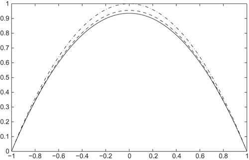
First, we present some results for the truth coupled system. In Figure 1, we show the truth macroscopic velocity field for the coupled system with at times t = 0, 0.5 and 1; note that the initial condition is identical to the uncoupled () steady-state velocity. The figure shows that the magnitude of the deviation from the Stokes velocity increases with time until it reaches a steady state and also that the presence of dumbbells increases effective viscosity.

Figure 1. The macroscopic velocity for the truth coupled Stokes Fokker–Planck system with at times (dash-dot line), (dashed line) and (solid line).

We then employ the reduced basis scheme for the coupled Stokes Fokker–Planck system with c = 0.1 and 0.2 and we use from Remark 4.1 (i.e. ). ³ In each case, we perform the POD–Greedy with and with three different values of TOL to generate reduced basis spaces of dimension N = 10, 20 and 30. Figure 2 shows the four basis functions constructed by the POD–Greedy algorithm in the case. We show in Table 1 the coupled error estimates as well as corresponding values of , the ‘true macroscopic error’ in the -seminorm at the final time , defined as

Figure 2. Basis functions 1, 2 and 10, 11 on the unit sphere for the Fokker–Planck equation generated by the POD–Greedy algorithm in the case. The basis functions generated earlier correspond to lower frequency modes.

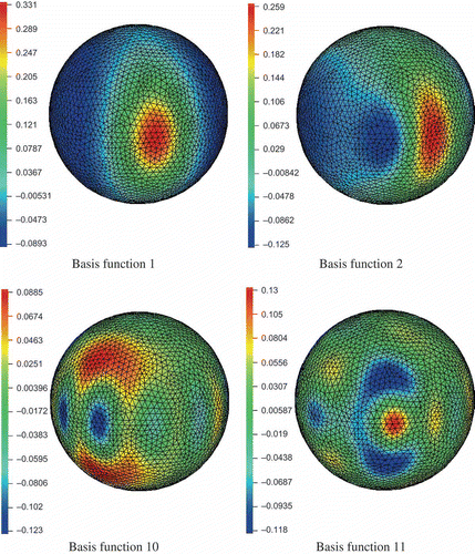
Table 1. Comparison of the macroscopic velocity error estimator and the true velocity error for and at the final time . The error estimator results were obtained with from Equation (33)(33) as a surrogate for

c	N
0.1	10	2.99e−3	4.04e−6
	20	1.04e−4	2.37e−8
	30	2.56e−5	7.82e−9
0.2	10	6.92e−1	8.51e−6
	20	3.60e−2	1.03e−7
	30	9.33e−3	1.44e−8

Table 1 shows that in practice overestimates the true error. This is primarily because the error analysis necessarily employs a ‘worst case’ growth rate that tends to be much larger than the growth rate of the true error. Moreover, is much more sensitive to the coupling constant than the true error – the sensitive dependence of on c follows from Equation (20)(20) where c enters into the exponential growth rate of the error estimate through . Nevertheless, the results in Table 1 show that for moderate values of c it is possible to ensure that is small in magnitude for the Poiseuille flow problem.

For the above results, the computation time for the truth coupled solve was 1595 seconds, and the reduced basis POD–Greedy computation time was 62, 130 and 203 seconds with N = 10, 20 and 30, respectively. We note also that a single coupled reduced solve is indeed very cheap: roughly 3.5 seconds with , 5 seconds with and 7 seconds with . All computations were performed on an AMD Opteron 248 processor. Finally, we note that the computational savings from the reduced basis approach would be much larger for two-dimensional or three-dimensional macroscopic flow domains in which could be orders of magnitude larger than considered here.

6. Conclusions

We have developed a new reduced basis framework for the coupled Stokes Fokker–Planck system for dilute liquid crystal flows. There are admittedly some limitations to our framework – most obviously our present lack of a rigorous a priori bound of the form (18) and also that tends to be a pessimistic estimate in practice. Nevertheless, the methodology in this article represents a promising first step in model reduction with quantitative error estimates for coupled multiscale systems of PDEs, and we intend to investigate the aforementioned shortcomings further in future work. The PGD approach has also been shown to be a powerful model reduction tool for multiscale polymeric fluid problems, especially for treating high-dimensional problems – the main advantage of our methodology, however, is that, as demonstrated in the numerical results section, our reduced order results are endowed with error estimates.

The reduced basis scheme presented here can be extended to more complex ‘non-parallel’ flows. The primary complication would be that each instantiation of the Fokker–Planck equation would be associated with a particle trajectory and hence we would require a Lagrangian scheme to track strain rate histories, but the essential character of our reduced basis scheme – and also our coupled error analysis – would carry over directly. We intend to consider complex macroscopic geometries in future work – indeed, the advantages of our reduced basis approach would be greatly amplified for large-scale problems in which would be much larger than the value considered in Section 5.

Another important extension would be to consider concentrated regimes in which excluded volume and dumbbell interaction effects are taken into account. This would necessitate a non-linear Fokker–Planck equation and would be a challenge from the point of view of rigorous error analysis – indeed, the derivation of rigorous RB error bounds for the non-linear Fokker–Planck equation without considering multiscale coupling effects is in itself a non-trivial task. As a result, to extend the results from this article to concentrated regimes, it may be necessary to employ non-rigorous error estimates in Algorithm 3.1, but it nevertheless seems possible that the RB approach presented here could be modified to perform well in this more difficult context.

Also, we note that in the model problem considered here, the rigid-rod dumbbells have a relatively small effect on the macroscopic velocity field. In situations where the polymer dynamics strongly influence the macroscopic velocity field, it is possible that we would need to consider some modifications to the ‘evolving training set’ strategy in Algorithm 3.1 to ensure that we obtain a robust method. For example, it could be important to consider ‘refreshing’ strategies, where we clear and restart the RB space training to prevent over-training on an ‘under-resolved’ velocity field. These issues will also be considered in future work.

Finally, we recall that the Stokes Fokker–Planck system is an example of a wider class of multiscale systems of PDEs, and hence advances in the error analysis for our model problem may be applicable in other contexts.

Acknowledgements

I thank Professor Anthony Patera of MIT for our many fruitful discussions on the material in this article. I acknowledge very helpful discussions with Professors Claude Le Bris and Sebastien Boyaval of the Ecole Nationale des Ponts et Chaussées, Professor Yvon Maday of University Paris VI and Professor Endre Süli of the University of Oxford. I also thank Professor Le Bris and Professor Maday for sharing a manuscript in preparation on a posteriori error bounds for multiscale problems. This work was supported by AFOSR Grant FA 9550-07-1-0425.

Notes

1.In future work, we intend to treat more complex flow geometries; by employing Lagrangian coordinates in the macroscopic domain, the transport term vanishes and we recover the formulation treated in this article, albeit with the extra complication of requiring a particle tracking scheme and where our time-dependent parameters become the velocity gradients associated with the particle trajectories.

2.In a similar manner, one can also show that is bounded below for arbitrary .

3.The choice is intended to be an ad hoc bound for for ; to confirm that is a conservative choice, we computed some sample values of and we observed that is typically roughly a factor of 10 smaller than the macroscopic error, . Hence, based on the results in Table 1 it is clear that is a very conservative bound for for the parameter choices considered here.

References

- Doi , M. and Edwards , S.F. 1986 . The Theory of Polymer Dynamics , Oxford : Clarendon Press .
- Bird , R.B. , Curtiss , C.F. , Armstrong , R.C. and Hassager , O. 1987 . Dynamics of Polymeric Liquids, Volume 2, Kinetic Theory , 2nd , New York : John Wiley and Sons .
- Helzel , C. and Otto , F. 2006 . Multiscale simulations of suspensions of rod-like molecules . J. Comp. Phys. , 216 : 52 – 75 .
- Chauvière , C. and Lozinski , A. 2004 . Simulation of complex viscoelastic flows using Fokker–Planck equation: 3D FENE model . J. Non-Newtonian Fluid Mech. , 122 : 201 – 214 .
- Chauvière , C. and Lozinski , A. 2004 . Simulation of dilute polymer solutions using a Fokker–Planck equation . Comput. Fluids , 33 : 687 – 696 .
- Lozinski , A. and Chauvière , C. 2003 . A fast solver for Fokker–Planck equation applied to viscoelastic flows calculation: 2D FENE model . J. Comput. Phys. , 189 : 607 – 625 .
- Knezevic , D.J. and üli , E. S . 2008 . A heterogeneous alternating-direction method for a micro-macro model of dilute polymeric fluids . Math. Model. Number. Anal. , 43 ( 6 ) : 1117 – 1156 .
- Bermejo , R. , Prieto , J.L. , Ilg , P. and Laso , M. 2009 . A stochastic semi-Lagrangian micro-macro model for liquid crystalline solutions . AIP Conference Proceedings , 1168 : 1259 – 1262 .
- Laso , M. and Öttinger , H.C. 1993 . Calculation of viscoelatic flow using molecular models: The CONNFFESSIT approach . J. Non-Newtonian Fluid Mech. , 47 : 1 – 20 .
- Öttinger , H.C. 1996 . Stochastic Processes in Polymeric Fluids , Berlin : Springer .
- Hua , C.C. and Schieber , J.D. 1996 . Application of kinetic theory models in spatiotemporal flows for polymer solutions, liquid crystals and polymer melts using the CONNFFESSIT approach . Chem. Eng. Sci. , 51 : 1473 – 1485 .
- Boyaval , S. and Lelievre , T. 2010 . A Variance Reduction Method for Parametrized Stochastic Differential Equations Using the Reduced Basis Paradigm . commun. math. sci. , 8 ( 3 ) : 735 – 762 .
- Bonvin , J. and Picasso , M. 1999 . Variance reduction methods for CONNFFESSIT-like simulations . J. Non-Newtonian Fluid Mech. , 84 : 191 – 215 .
- Jourdain , B. , Le Bris , C. and Lelievre , T. 2004 . On a variance reduction technique for micro-macro simulations of polymeric fluids . J. Non-Newtonian Fluid Mech. , 122 : 91 – 106 .
- Ammar , A. , Mokdad , B. , Chinesta , F. and Keunings , R. 2006 . A new family of solvers for some classes of multidimensional partial differential equations encountered in kinetic theory modeling of complex fluids . J. Non-Newtonian Fluid Mech. , 139 : 153 – 176 .
- Ammar , A. , Mokdad , B. , Chinesta , F. and Keunings , R. 2007 . A new family of solvers for some classes of multidimensional partial differential equations encountered in kinetic theory modelling of complex fluids. Part II: Transient simulation using space-time separated representations . J. Non-Newtonian Fluid Mech. , 144 : 98 – 121 .
- Pruliere , E. , Ammar , A. , El Kissi , N. and Chinesta , F. 2008 . Recirculating flows involving short fiber suspensions: Numerical difficulties and efficient advanced micro-macro solvers . Arch. Comput. Methods Eng. , 16 : 1 – 30 .
- Knezevic , D.J. and Patera , A.T. 2010 . A certified reduced basis method for the Fokker–Planck equation of dilute polymeric fluids: FENE Dumbbells in extensional flow . SIAM J. Sci. Comput. , 32 : 793 – 817 .
- Rozza , G. , Huynh , D.B.P. and Patera , A.T. 2008 . Reduced basis approximation and a posteriori error estimation for affinely parametrized elliptic coercive partial differential equations: Application to transport and continuum mechanics . Arch. Comput. Methods Eng. , 15 : 229 – 275 .
- Huynh , D. , Rozza , G. , Sen , S. and Patera , A. 2007 . A successive constraint linear optimization method for lower bounds of parametric coercivity and inf-sup stability constants . Comptes Rendus Mathematique , 345 : 473 – 478 .
- Barrault , M. , Maday , Y. , Nguyen , A.T. and Patera , N.C. 2004 . An ‘empirical interpolation’ method: Application to efficient reduced-basis discretization of partial differential equations . Comptes Rendus Mathematique , 339 : 667 – 672 .
- Haasdonk , B. and Ohlberger , M. 2008 . Reduced basis method for finite volume approximations of parametrized linear evolution equations . Math. Model. Numer. Anal. , 42 : 277 – 302 .
- Gunzburger , M.D. 2003 . Perspectives in Flow Control and Optimization , Berlin : SIAM Publications .
- Cazemier , W. 1997 . Proper orthogonal decomposition and low dimensional models for turbulent flows , Ph.D. Thesis, University of Groningen .