Model order reduction and error estimation with an application to the parameter-dependent eddy current equation

Abstract

In product development, engineers simulate the underlying partial differential equation many times with commercial tools for different geometries. Since the available computation time is limited, we look for reduced models with an error estimator that guarantees the accuracy of the reduced model. Using commercial tools the theoretical methods proposed by G. Rozza, D.B.P. Huynh and A.T. Patera [Reduced basis approximation and a posteriori error estimation for affinely parameterized elliptic coercive partial differential equations, Arch. Comput. Methods Eng. 15 (2008), pp. 229–275] lead to technical difficulties. We present how to overcome these challenges and validate the error estimator by applying it to a simple model of a solenoid actuator that is a part of a valve.

Keywords:

• model order reduction
• Krylov subspace method
• reduced basis method
• a posteriori error estimator
• eddy current equation

1. Introduction

Model order reduction methods are effective methods that reduce the computational complexity of partial differential equations (PDEs) and dynamical systems, respectively. In literature many different reduction methods have been presented. Here, we focus on the reduced basis method (RBM) and Krylov subspace methods. The RBM is discussed in detail in [1,2]. The basics of the local and global Krylov subspace methods are introduced in [3–6].

In this article, we combine the ingredients of the RBM with the Krylov subspace methods and compare them. Additionally, we adapt the error estimator from [2, Section 4.4] and derive an ‘optimized’ L ²-error estimator that reduces the increase of the effectivity with the time compared to a simpler L ²-error estimator.

In general, the theory is applicable to linear PDE or linear dynamical systems with geometrical parameters. As an example, we treat the eddy current equation in the time domain. All error estimators are applied to the eddy current equation in connection with the RBM, and the global and local Krylov subspace method. Afterwards, the three reduction methods are compared. To the best of our knowledge, we provide with this the first comparison of Krylov subspace methods and the RBM. Also, the application of efficient a posteriori error estimates to the Krylov subspace methods is considered a main contribution.

The outline of this article consists of model order reduction and error estimation. The basics are given in Section 1. We present a strategy to exactly interpolate the dynamical matrices in Section 2. A posteriori error estimators are derived in Section 3. Then, different reduction methods are proposed in Section 4. An offline–online decomposition is described in Section 5. Finally, we compare and summarize the results in Section 6.

1.1. Partial differential equation formulation

In practice, the eddy current equation is used to design electromagnetic devices such as solenoid actuators. The eddy current equation,

(1)

describes the propagation of an electromagnetic field. The unknown is the vector potential for all , stands for the magnetic reluctivity and the scalar represents the input current. Geometrical parameters are involved by a parameter-dependent domain . The parameter is . We assume linear materials, that is does not depend on . The time is discretized by the Backward Euler scheme with time step . The time span is replaced by a set of equidistant time instants and the time derivative by its finite difference quotient. For simplicity, we set , if confusion is unlikely. Then, the semidiscrete weak form is

(2)

with and the function space

(3)

The inner product is defined as with the reference domain , while is the reference domain corresponding to the anchor. Consequently, the induced norm is . The parameter-dependent bilinear forms are and with

(4)

The constant represents the conductivity. The bilinear form contains the boundary element integrals (see [7] for details). The theoretical background of the time-independent eddy current equation in two dimensions is discussed in [8]. While the RBM is based on the weak formulation in bilinear forms (Equation (2)(2)), the Krylov subspace method is adapted from the state space formulation. Therefore, we introduce the appropriate state space formulation in Section 1.2.

1.2. State space formulation

The space is discretized by the finite element method (FEM). The finite element (FE) space is of finite dimension, . After space discretization, Equation (1)(1) can be reformulated as the state space system

(5)

with the unknown . In detail, the matrices as well as are , and with . The FE basis functions span the space that is, . The FE approximation is . The dimension and therefore the simulation time is increasing with the accuracy of the FE approximation. In practice, we want to reduce the simulation time but guarantee that a given accuracy is fulfilled. In Section 1.3 we present a technique that reduces the simulation time and afterwards we introduce a posteriori error estimators that guarantee the accuracy.

1.3. Reduction

Our goal is to reduce the computational complexity and guarantee the accuracy of the reduced approximation. While the FE solution is contained in a high-dimensional space , the reduced approximation belongs to a lower dimensional space, . The space can be constructed by different reduction methods, see Section 4. The original equation is projected via Ritz Galerkin to a lower dimensional space. Given , we look for such that

(6)

subject to the initial condition . In detail, with the reduced basis functions . After reducing the state space system corresponding to Equation (6)(6) for the unknown vectors is

(7)

2. Affine decomposition

The so-called affine decomposition is necessary to reduce the computational complexity by an offline–online decomposition. An affine decomposition consists of parameter-independent forms or matrices and parameter-dependent factors. Considering the bilinear form , we look for an affine decomposition

(8)

The parameter-dependent factors are , while the parameter-independent matrices are for all . Our goal is to construct an affine decomposition of the bilinear forms (Equation (4)(4)) or matrices, respectively. Moosmann proposed in [9, Sections 2.4, 5.2.2] an approach to assemble the system matrices for geometrical parameters. Here, we apply a more general strategy. The idea is to introduce a reference domain and an affine mapping and for each domain a transformation with

(9)

The parameter-dependent mapping represents modifications of the geometry. In detail the vector translates the reference geometry, while the matrix scales the reference geometry. In [10, Sections 5.1, 5.2] Rozza et al. described how to obtain an affine decomposable bilinear form with the parameter-dependent mapping defined in Equation (9)(9).

Remark 1

(BEM part of the system matrix)

In addition to the bilinear form , the system matrix , or the bilinear form , contains a boundary element method (BEM) contribution, that is, . The BEM part is interpolated with a negligible error, that is, .

Remark 2

(Mass matrix and right-hand side)

Analogous to the stiffness matrix , the mass matrix in Equation (5)(5) is interpolated exactly, with . Furthermore, the corresponding bilinear form can be decomposed as . The right-hand side vector is also interpolated exactly, that is, or for the linear form .

2.1. Simple example

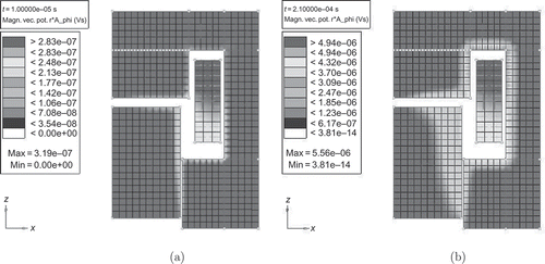
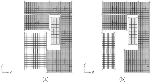
The geometry of interest is visualized in Figure 1 (a) and (b), while the field variables at first and last time step, that is, and are given in Figure 2. The components of the valve are the anchor (light grey), the core (dark grey) and the coil (grey) (see Figure 1). The only varying geometry is the width of the anchor, that is, and . As a parameter variation, we vary the width of the anchor, from mm, see Figure 1 (a), up to 10 mm, see Figure 1 (b). The mapping of Equation (9)(9) yields with

(10)

and and . We compute the FE matrices for mm via an interpolation and compare it to the one exported from the commercial tool. The maximum relative error in the matrix entries is .

Figure 2. Magnetic vector potential at the initial time s and final time .

Figure 1. Example of different geometries of a valve: (a) the reference domain and (b) the varied geometry – the anchor is scaled.

3. A posteriori error estimation

The a posteriori error bound serves to check the accuracy of the reduced approximation and is efficiently computable. In [11] the ideas of the RBM have been adapted to dynamical systems. A posteriori error bounds are an essential ingredient of the RBM (see [1] for further references). In [12] error bounds for systems reduced by proper orthogonal decomposition (POD) are presented. To the best of our knowledge, we firstly present an error estimator for Krylov subspace methods. Initially, we define the main ingredients. Then, we derive the energy-, L ²- and optimized L ²-error bounds. In Section 5 the computation of the error estimators is described.

3.1. Introductory definitions

For the primal residual is ,

(11)

for all and in the dual norm it is

(12)

The energy norm and the L ²-norm are defined for all as

(13)

and the L ²-norm as

(14)

for a fixed parameter mm. The effectivity is defined as the error estimator divided by the real error in the corresponding norm,

(15)

where denotes the error estimator in the energy norm which will be defined in Section 3.2. Similar to Equation (15)(15) the effectivities for the L ²-norms are

(16)

with the L ²-norm error estimator and , respectively, which are defined in the Section 3.2.

Definition 3.1

Coercivity and Continuity Constants

The coercivity constants of the bilinear form and are defined as

(17)

with respect to and . The continuity constant with respect to is

The lower bounds for the coercivity constants are and . Analogously, the upper bound for the continuity constant is .

The lower bounds for the coercivity constants are computed via a ‘ min’ approach (see [1, Section 4.2.2] for details).

Remark 3

Properties of the bilinear forms (Equation (4)(4))

The bilinear forms (Equation (4)(4)) are coercive and continuous, since as well as are positive and is continuous and coercive with respect to (see [8, Theorem 2.6] for details). Hence, the coercivity with respect to is a consequence of the Poincare inequality (see [13]). The bilinear form is coercive with respect to , since is positive.

3.2. Energy norm estimator

The error bound presented in this section estimates the error between the full-order field variable and the reduced in the energy norm (Equation (14)(14)). We adapt the error estimator derived in [2, Section 4.4] to the eddy current equation. In the following we will present the proof in detail, as it will be modified for further estimators.

Proposition 3.2

Let be the error in the field variable, then

(18)

holds for all with the constants and of Definition 3.1.

Proof

The basic idea of the proof is to subtract the primal residuum in Equation (11)(11) from the original Equation (2)(2). Setting and exploiting the Cauchy–Schwarz inequality for yields

(19)

Afterwards, we apply the Young inequality, , twice, with and , that is,

(20)

Inserting Equation (20)(20) in Equation (19)(19) results in

(21)

Multiplying by 2 and using that holds, we obtain

(22)

Finally, we replace k by and sum over all times, . Exploiting the telescope sum trick and completes the proof.

Similar to Proposition 3.1, we can derive an error bound for the L ²-norm (Equation (14)(14)).

Proposition 3.3

(L ² -error estimator) Let be the full-order solution and the reduced approximation, then the error can be estimated by

(23)

with the constants from Definition 3.1.

Proof

We recall the first steps of the proof of Proposition 3.2. Setting and , Equation (20)(20) in the proof of Proposition 3.2 yields

(24)

Using and multiplying by 2 results in Equation (25)(25)

(25)

Afterwards, we replace k by and apply the telescope sum trick:

(26)

Finally, we use the predefined constants, that is, .

3.3. Optimized L²-estimator

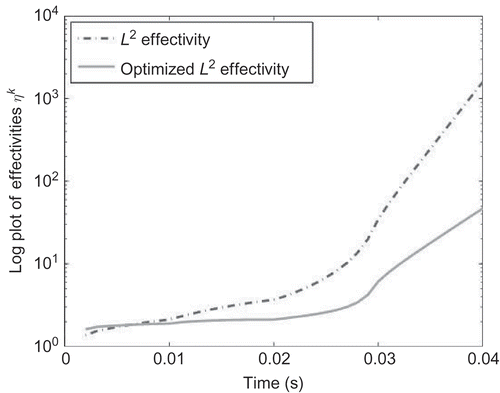
In Figures 5, 8 and 11, it will be demonstrated that the effectivity of the L ²-norm estimator is increasing with time. In practice, this means that the overestimation of the error estimator compared to the real error grows with the time. The optimized L ²-norm bound reduces the increase of the effectivity with the time.

Figure 11. The effectivities for the L ²- and optimized L ²-error estimators with the local Krylov subspace method, and for mm are visualized.

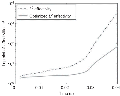
Figure 5. The effectivities for the L ²- and optimized L ²-error estimators in connection with the RBM, and for mm are visualized.

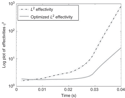
Figure 8. The effectivities for the L ²- and optimized L ²-error estimators related to the global Krylov subspace method, and for mm are visualized.

Proposition 3.4

Let the constants and from Definition 3.1 be given. Then for all , the error can be estimated as

(27)

Proof

We recall Equation (22)(22). The left-hand side of Equation (22)(22) is estimated by

(28)

Inserting Equation (28)(28) in Equation (22)(22) and multiplying the whole inequality with yields

(29)

Setting and invoking the telescope sum trick , we obtain

(30)

Using and dividing by results in Equation (27)(27).

4. Reduction methods and their application

In this section, we introduce three different reduction methods: the RBM, the global and the local Krylov subspace method. The error estimators derived in Section 3 are applicable in connection with all reduction methods.

4.1. The RBM with the POD–greedy algorithm

In the RBM context the lower dimensional space contains N -orthonormal basis functions , . The reduced basis space is constructed by the POD–Greedy Algorithm, presented in [11, Section 6] and [14, Section 4.2]. Let be the full-order trajectory and the snapshot matrix for the end–time index K and the parameter . Analogously, the reduced trajectory is .

4.1.1. Proper orthogonal decomposition

The POD method is used to find a lower dimensional approximation to the space spanned by the snapshot matrix , see [15] for details. We use a matrix with the inner product . The matrix is symmetric and therefore the eigenvalues and eigenvectors of the eigenvalue problem are real and orthogonal with respect to the inner product, that is, is diagonal. After the Mth column we truncate the eigenvector matrix , . The data matrix is projected by , that is, . Finally, the reduced data matrix is normalized, . Let denote the M largest POD modes of the data matrix with respect to the inner product .

4.1.2. Sampling procedure

The parameter sample set for the problem is defined as a set of parameters and constructed by the POD–Greedy algorithm. is a training set of points in . The set is initialized with an arbitrarily chosen , that is, and . The maximal dimension of the reduced space is . In each step we add basis functions to the reduced space.

1.	While the offline quantities, see Section 5 for details, are computed and then the reduced approximations as well as the error estimator are computed for all . The computation of and for all is fast and independent of the size of the full model, .
2.	Next, we identify the parameter with the largest error estimator for . Alternatively, we can find the maximum argument for the normalized error over the training set, that is, For this parameter , we evaluate the full-order trajectory and the project to the existing reduced basis space with respect to the inner product . The -orthogonal part of is saved in for .
3.	Afterwards, we select the -dominating modes of and add these modes to the existing reduced basis space, that is, , and .

4.1.3. Numerical results

The underlying example is the simple valve introduced in Section 2.1. The parameter domain is and the training sample set is

We set and as a result of the POD–Greedy algorithm the parameter sample set we obtain

Note that if a parameter is chosen more than once, we add the two or more dominating modes of the system corresponding to this parameter in the POD–Greedy algorithm.

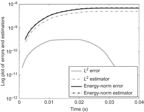
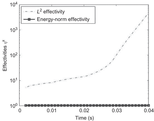
In Figure 3, the energy norm and the L ²-error estimator as well as the real errors are visualized for the parameter of interest, mm. In Figure 4 the L ²-norm effectivity is highly increasing, while the energy-norm effectivity is not. Using the optimized L ²-norm, the effectivity is decreasing with respect to the L ²-norm effectivity (see Figure 5).

Figure 3. The error estimator and for mm are plotted. The system is reduced by the RBM with the POD–Greedy algorithm and .

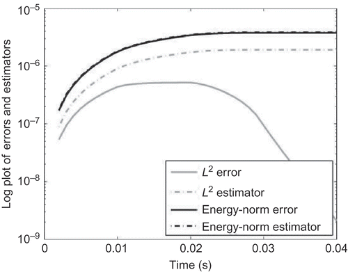
Figure 4. The effectivities for mm are plotted. The system is reduced by the RBM with the POD–Greedy algorithm and .

In Table 1, the value of the errors and its estimators for different reduced orders N, that is, and 20, is presented. By increasing the reduced order the errors and its estimators are decreasing, but the CPU time is increasing. Table 2 shows that we save CPU time up to 14.302 s, if we evaluate the reduced approximation and the error estimator instead of the full-order solution. In conclusion, we have a speed-up factor of 239.4, that is, we save of the CPU time by computing the reduced model together with the error estimator. The only effort we need to spend is the offline computation which in this case will take 236.855 s. But once we evaluated the offline quantities, we are able to compute the reduced approximation and the error estimator efficiently for any parameter configuration within the given domain, .

Table 1. Error estimator and efficiency for the POD–Greedy RBM

N
5
10
20
Note: The error estimator and real error for different N.

Table 2. CPU times – POD–Greedy RBM

N	Offline
5	236.855	0.031	0.019	14.362
10	258.36	0.038	0.024	14.362
20	298.192	0.04252	0.025	14.362
Note: The CPU times for the offline and online stage.

4.2. Krylov subspace method

The Krylov subspace method constructs the lower dimensional space by the Krylov subspaces, that is, the qth order input Krylov subspace is

(31)

with the system matrices and of Equation (5)(5) (see [3] for details).

We consider I different reference parameters , . The matrices of the parameter-dependent system are denoted by , and for . The local Krylov subspaces with expansion point are

(32)

Remark 4

Analogous to the RBM a greedy algorithm (see Section 4.1) might be used to choose the reference parameters for the local models. This might be discussed in future work.

4.2.1. Global Krylov subspace method

The global Krylov subspace method is also known as the implicit moment matching algorithm [9, Section 4.3]. Using the global Krylov subspace method for the reduction of a parameter-dependent system, the reduced space is constructed as a set of input Krylov subspaces. The global Krylov subspace is . In order to avoid redundant basis functions, we perform a singular value decomposition of , that is, . The first N columns of U build the global projection matrix . Since the full-order system matrices are affinely decomposable, that is, , offline we project the parameter-independent matrix , that is, . Online we evaluate the factor for a new parameter and . The assembly of the reduced matrix is done online, too. Similar to the matrix , the reduced matrices and are constructed. Analogous to the RBM, the a posteriori error estimators from Section 3 can be adapted. In order to get an offline–online decomposition of the system matrices, we apply the matrix interpolation strategy proposed in Section 2.

4.2.2. Local Krylov subspace method

Compared to the global Krylov subspace method, the local Krylov subspace method interpolates I reduced models. To guarantee the compatibility of the local coordinate systems according to [4], we introduce the matrix . After setting , a singular value decomposition yields . In order to capture the N most important directions, the matrix R consists of the first columns of U. Each locally reduced system is projected via a state transformation , so that all reduced models are compatible and have the same physical interpretation. For instance, the reduced matrix is . The weighting functions switch smoothly between the different models. Hence, the reduced system is

(33)

with .

4.2.3. Error estimators

The error estimators from Section 3, Propositions 3.2–3.4, are applicable in connection with the local Krylov subspace method.

Since the projection matrix is parameter dependent, we define the discrete primal residual from Equation (11)(11)

(34)

Using the inner-product matrix and Equation (34)(34), the dual norm of the primal residual yields In practice, the dual norm of the primal residual is computed via an offline–online computation.

4.2.4. Numerical results

The reference parameters are and the weighting functions are first-order Lagrange functions .

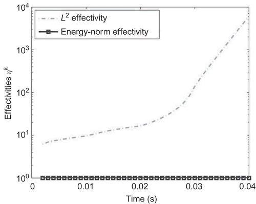
In Figure 6 the energy- and L ²-norm estimators for the global Krylov subspace method are plotted. The effectivities for the global Krylov subspace method are shown in Figures 7 and 8.

Figure 6. The error estimators , for mm are plotted. The system is reduced by the global Krylov subspace method with .

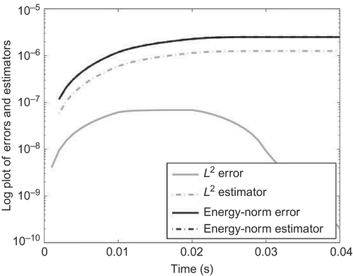
Figure 7. The effectivities for mm are plotted. The system is reduced by the global Krylov subspace method with .

The maximal overestimation of the local Krylov subspace method is a factor 4 in the energy norm, see Figure 9. The error estimators and the real errors of the local Krylov subspace method are visualized in Figure 10.

Figure 10. Local Krylov Subspace Method: Error estimators , for mm are visualized.

Figure 9. Local Krylov Subspace Method: The effectivities for mm are visualized.

Using the reduced model constructed by the global Krylov subspace method, we save CPU time up to 14.35 s. This means we have a speed-up factor up to 1186.9 (see Table 3). The local Krylov subspace method enables the user to save CPU time up to 14.35 s and achieves a speed-up factor up to 649.86 (see Table 4). The L ²-norm effectivity is up to 1000. This means that the real error is overestimated by a factor 1000. In order to reduce the overestimation of the L ²-norm, we derived the optimized L ²-norm. Its result is visualized in the Figures 8 and 11. Compared to the global Krylov subspace method, the local one is faster than the global one. The accuracy of the local Krylov subspace method is up to a factor 10 higher than the global one (see Tables 5 and 6). Tables 5 and 6 additionally demonstrate that the errors are decreasing, while the reduced order is increasing.

Table 3. CPU times – global Krylov subspace method

N	Offline
10		0.0004	0.016	14.364
20		0.0015	0.017	14.364
50		0.0023	0.028	14.364
100		0.0052	0.035	14.364
Note: The CPU times for the offline and online stages.

Table 4. CPU times – local Krylov subspace method

N	Offline
10	50.346	0.0006	0.0215	14.362
20	68.435	0.0019	0.0284	14.362
50	167.402	0.003	0.0367	14.362
100	256.316	0.0082	0.0388	14.362
Note: The CPU times for the offline and online stages.

Table 5. Error estimator and efficiency for the local Krylov subspace method

N
10
20
50
100
Note: The error estimator and normalized error estimator for different N.

Table 6. Error estimator and efficiency for the global Krylov subspace method

N
10
20
50
100
Note: The error estimator and normalized error estimator for different N.

5. Offline–online procedure

In this section, we exploit that the system matrices are affine decomposable. The main idea to gain fast models is to decompose the computational effort in an offline stage and an online stage. The offline stage is only performed once and contains expensive operations, while the online stage is performed for every new parameter configuration. The online stage is inexpensive, because the computational complexity is independent of . Both the reduced approximation and the error estimators are evaluated via an online and an offline stage. Reducing the system by RBM, we first construct an affine decomposition of the bilinear forms or system matrices. Inserting the affine decomposition in Equation (6)(6), the reduced system for all is

(35)

The matrices and corresponding to the bilinear forms , and are computed offline. The parameter-dependent factors and as well as and the reduced approximation are evaluated online.

Considering the computational complexity of the local Krylov subspace method, offline we build the local Krylov subspaces as well as the transformation matrices and reduce the local system matrices. Then, we construct the affine decomposition of the matrices. Offline we compute the locally reduced and transformed matrices. Online we evaluate the weighting functions and interpolate the local models to get the reduced system matrices. Afterwards, we compute the reduced approximation.

Analogous to the reduced approximation, the error estimator is computed via an online–offline decomposition. The error estimator consists of particular constants from Definition 3.1 and the dual norm of the primal residual as well as the initial error in the L ²-norm. The constants involved in the error estimator are computed via a -min approach. The initial error is computed once offline. The dual norm of the primal residual can be decomposed efficiently. After using the Riesz representation theorem, we have that fulfils

(36)

The standard duality argument results in

(37)

The residual contains the bilinear forms that are decomposable. Combining Equations (36)(36) and (37) yields

(38)

The time step is involved in . For , we compute offline

(39)

where is the inner-product matrix to . The parameter-independent matrices are and for . Here, the indicates that the quantity is evaluated offline. Considering the local Krylov subspace method, the factors and so on are re-defined as and so on for all . The parameter-dependent factors also involves the weighting functions .

Remark 5

(More Parameters) If we consider more than one parameter, the offline and online effort can increase significantly. Using the h–p techniques proposed in [16] we can make the online stage arbitrarily fast, but on the other hand the offline computational complexity is increasing. The offline effort can be reduced by adaptive training samples, see [17] for details.

6. Conclusion

6.1. Comparison

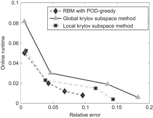
The advantages of the Krylov subspace methods are that no pre-computations of the full-order system are needed, while the RBM uses the pre-computed snapshots. Additionally, the Krylov subspace methods do not depend on the input . The RBM is based on the PDE. Therefore, it provides the opportunity to incorporate more details, for example, the appropriate inner product into the reduction. In order to compare the different reduction methods, we plot the maximum energy-norm error over a test set of parameters with respect to the online runtime. Here, the arbitrarily chosen test set is . Compared to the global Krylov subspace method, the local one and the RBM are more accurate for the same online runtime (see Figure 12). In comparison, the global Krylov subspace method is slower, if we need to guarantee a given accuracy. Comparing the RBM with the local Krylov subspace method (see Figure 12), the RBM is minimal faster or more accurate, respectively.

Figure 12. Comparison of the methods.

6.2. Summary

On the one hand, three reduction methods are compared, the well-established RBM, the global Krylov subspace method and a newer approach, the local Krylov subspace method. On the other hand, the error estimators presented in [2] are applied in connection with all three methods. Additionally, a new error estimator, an optimized L ²-error estimator, is proposed and applied. In general, the proposed estimators are applicable for linear dynamical systems or linear PDEs with geometrical parameters or affinely decomposable bilinear forms. To our knowledge, it is the first approach presenting an error estimator for the global and local Krylov subspace methods.

A realistic example shows the applicability to physical problems. The examples demonstrate that the online effort of all three methods is comparable. In particular, the global Krylov subspace method is slightly slower or less accurate, respectively. In addition, the example demonstrates that the effectivity is reduced with respect to the time. Furthermore, we accomplished an affine decomposition for commercial tools. In future work we focus on non-linear problems and more varying parameters.

Acknowledgements

We thank O. Rain of the Robert Bosch GmbH; D.J. Knezevic, J. Lohne-Eftang and D.B.P. Huynh of MIT (Department of Mechanical Engineering); and M. Grepl (RWTH Aachen), K. Veroy-Grepl (RWTH Aachen) as well as R. Eid of the TUM (Technical University Munich) for their fruitful discussions and advice. The first author is a member of the TUM Graduate School.

References

- Patera , A.T. and Rozza , G. Reduced Basis Approximation and A Posteriori Error Estimation for Parameterized Partial Differential Equations . Copyright MIT 2006, to appear in MIT Pappalardo Graduate Monographs in Mechanical Engineering, 2007. University of Bremen . Bremen.
- Grepl , M. 2005 . Reduced-Basis Approximations and a Posteriori Error Estimation for Parabolic Partial Differential Equations , Cambridge, MA : Massachusetts Institute of Technology .
- Salimbahrami , B. and Lohmann , B. Krylov subspace methods in linear model order reduction: introduction and invariance properties . Sci. Rep. NR2, Institute of Automation, University of Bremen . Bremen.
- Panzer , H. , Mohring , J. , Eid , R. and Lohmann , B. 2010 . Parametric model order reduction by matrix interpolation , 58 : 475 – 484 . Automatisierungstechnik
- Antoulas , A.C. 2005 . Approximation of Large-Scale Dynamical Systems , Philadelphia, PA : SIAM .
- Lohmann , B. and Eid , R. 2009 . “ Efficient order reduction of parametric and nonlinear models by superposition of locally reduced models ” . In Methoden und Anwendungen der Regelungstechnik , Edited by: Roppencker , G. and Lohmann , B. 27 – 37 . Munich : Hrsg., Erlangen-Münchener Workshops 2007 und 2008, Technical University of Munich .
- Rischmüller , V. 2004 . Eine Parallelisierung der Kopplung der Finite Elemente Methode und der Randele-mentmethode , Germany : Universtitát Stuttgart .
- Pechstein , C. 2004 . Multigrid-Newton-Methods for Nonlinear Magnetostatic Problems , Austria : University of Linz .
- Moosmann , C. 2007 . ParaMOR – Model order reduction for parameterized MEMS applications , Germany : Ph.D. thesis, IMTEK .
- Rozza , G. , Huynh , D.B.P. and Patera , A.T. 2008 . Reduced basis approximation and a posteriori error estimation for affinely parameterized elliptic coercive partial differential equations . Arch. Comput. Meth. Eng. , 15 : 229 – 275 .
- Haasdonk , B. and Ohlberger , M. 2008 . Reduced basis method for finite volume approximations of parameterized evolution equations . M2AN, Math. Model. Numer. Anal. , 42 : 277 – 302 .
- Volkwein , S. 2008 . Model Reduction using Proper Orthogonal Decomposition , Austria : Lecture notes, University of Graz .
- Evans , L.C. 1998 . Partial Differential Equations , Providence, RI : American Mathematical Society .
- Knezevic , D.J. and Patera , A.T. 2010 . A certified reduced basis method for the Fokker-Planck equation of dilute polymeric fluids: fene dumbells in extensional flow . SIAM J. Sci. Comput. , 32 ( 2 ) : 793 – 817 .
- Volkwein , S. 2001 . Optimal and Suboptimal Control of Partial Differential Equations: Augumented Lagrange-SQP Methods and Reduced-Order Modeling with Proper Orthogonal Decomposition , Austria : Institute of Mathematics, University of Graz .
- Eftang , J.L. , Knezevic , D.J. and Patera , A.T. An hp certified reduced basis method for parametrized parabolic partial differential equations . preprint (2011), to appear in Math. Comput. Model. Dyn. Syst. ,
- Haasdonk , B. and Ohlberger , M. Adaptive basis enrichment for the reduced basis method applied to finite volume schemes . Proceedings of 5th International Symposium on Finite Volumes for Complex Applications . pp. 471 – 478 . Münster : University of Münster .
- Haasdonk , B. and Ohlberger , M. 2009 . Efficient reduced models and a-posteriori error estimation for parameterized dynamical systems by offline/online decomposition . Sim Tech Preprint 2009–23 ,
- Albunni , N. , Rischmüller , V. , Fritzsche , T. and Lohmann , B. 2009 . Multiobjective optimization of the design of nonlinear electromagnetic systems using parametric reduced order models . IEEE Tran. Magn. , 45 ( 3 ) : 1474 – 1477 .
- Albunni , N. , Eid , R. and Lohmann , B. Model Order Reduction of Electromagnetic Devices with a Mixed Current-Voltage Excitation . Proceedings of MATHMOD . Vienna, Austria.
- Huynh , D.B.P. , Rozza , G. , Sen , S. and Patera , A.T. 2007 . A successive constraint linear optimization method for lower bounds of parametric coercivity and inf-sup stability constants . CR Acad. Sci. Paris Ser. I , 345 : 473 – 478 .
- Chen , Y. , Hesthaven , J.S. , Maday , Y. and Rodriguez , J. 2007 . Certified reduced basis method and output bounds for the harmonic Maxwell's equations . SIAM J. Sci. Comput. , 32 ( 2 ) : 970 – 996 .
- Fares , M. , Hesthaven , J.S. , Maday , Y. and Stamm , B. 2010 . The Reduced Basis Method for the Electric Field Integral Equation , Providence, RI : Brown University .